Interface stability in granular open filters in unidirectional flows: investigating the required minimum filter layer thickness for stable geometrical open filters in unidirectional flows

(1)

Interface stability in granular open filters in

unidirectional flows

Investigating the required minimum filter layer thickness

for stable geometrical open filters in unidirectional flows.

Report type: Author: Date:

Graduation committee:

MSc Thesis R. Joustra April 2013

Dr. J.J. Warmink (University of Twente) Dr. Ir. C.M. Dohmen-Janssen (University of Twente) Ir. B. de Sonneville (Deltares)

Ir. H.J. Verheij (Deltares)

(2)

(3)

MSc thesis Page 3

Summary

A single-grading stable geometrical open filter is a measure of granular material to protect a bed or construction against scour and erosion. A stable geometrical open filter must have a sufficiently large filter diameter to prevent the shear failure (Chiew, 1995) and a sufficiently large relative layer thickness to prevent transport of bed material through the pores of the filter (winnowing failure (Chiew, 1995)). This thesis focuses on the interface stability in a unidirectional current, e.g. prevention of the transport of bed material through the pores of the filter. The design formula of Hoffmans (2012) can be applied to calculate the minimum required layer thickness to prevent winnowing. This formula is based on the philosophy of simultaneous erosion of the filter material and the bed material, e.g. filter material and bed material are eroded at the same external load conditions. Load damping coefficientαd within the formula of Hoffmans

(2012) is the parameter which describes turbulent kinetic energy damping by the filter. The value for αd

should be increased when the minimum filter layer thickness is insufficient to prevent winnowing.

Van de Sande (2012) recently modified the formula and concluded that the formula is valid for uniform flow conditions. Theoretically the formula is also valid for non-uniform flow (e.g. conditions with additional turbulence) (Hoffmans, 2012), however this has not yet been confirmed with laboratory experiments. Firstly, indicatory results by Van de Sande (2012) show that bed mobility increases for conditions with additional turbulence (non-uniform flow). Secondly, a few results of laboratory tests by Van Velzen (2012) indicated a probable validity of flow with a cylindrical pier (non-uniform flow). Thirdly, Wörman (1989) developed a similar design formula for the layer thickness of geometrical open filters in flows with a cylindrical pier. The similarity of the design formula of Wörman (1989) and Hoffmans (2012) is the design philosophy of simultaneous erosion of filter and bed material. The main difference is that Wörman found a linear relation between the filter and bed grain characteristics and the minimum filter layer thickness, while Hoffmans (2012) described that relation with a logarithmic function. The formula of Wörman is based on experiments of flow at a cylindrical pier and is only tested for small layer thicknesses (Df <0.1 m) and low flow velocities (ū < 0.5 m/s).

Recently, a database became available with experiments performed by Joustra (2012) and conducted at the research institute Deltares. The test data give the possibility to test the validity of the by Van de Sande (2012) modified version of the formula of Hoffmans (2012) for (1) uniform flow, and for non-uniform flow conditions in cases of (2) sill-induced additional turbulence and (3) flow with a cylindrical pier. In addition, the database provides the possibility of testing the validity of the formula of Wörman (1989) for flow velocities over 0.5 m/s and layer thicknesses over 0.1 m at the cylindrical pier. The aim of this thesis is: To test the validity of the design formula of Hoffmans (2012) for flows with sill-induced additional turbulence, and flows with a cylindrical pier and to test the validity of the design formula of Wörman (1989) for flow velocities over 0.5 m/s and filter layer thicknesses over 0.1 m at flows with cylindrical piers.

First, the tests conducted by Joustra (2012) are redistributed into flow categories (1) uniform flow, (2) flows with sill-induced additional turbulence and (3) flows with a cylindrical pier. Second, the filter material instability and bed material instability are classified separately. This separate classification is determined for each test with visual observation using underwater camera images and processed videos. Third, the separate classification is combined into a general classification. In addition, the bed material instability classification is verified with 3D Stereo photography images for conditions (1) and (2). The simplified (αd = 0.86) and full version (αd = 0.82)of the formula of Hoffmans (2012) are compared with the

(4)

MSc thesis Page 4

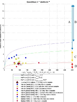
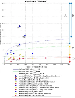
First, the data of Joustra (2012) with condition of uniform flow are in agreement with the formula of Hoffmans (2012) with the load damping coefficient αd = 0.82 for the full version and αd = 0.86 for the

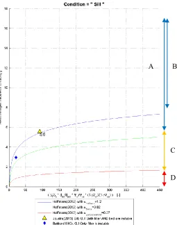
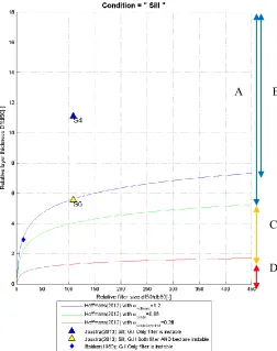
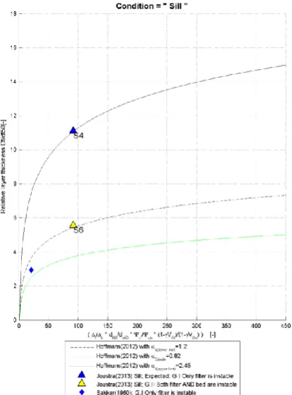
simplified version. This result is based on one single test that could be classified and selected for validation and an expected classification of three additional tests when the flow velocity would have been further increased. Second, the data of Joustra (2012) with flows with sill-induced additional turbulence suggest to increase the load damping coefficient αd = 0.82 for the full version and the αd = 0.86 for the simplified

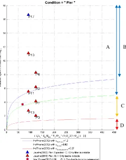
version of the formula of Hoffmans (2012). A rough estimate of the new load damping coefficient for both versions of the formula and flows with sill-induced additional turbulence is probably within the range 1.2 < αd < 2.5, but additional research is highly recommended due to the uncertainty in results and scarcity of

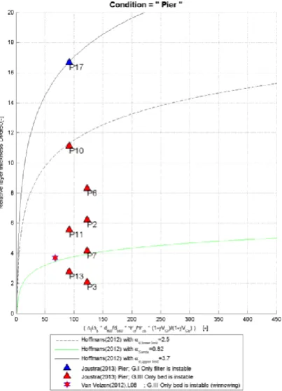
tests. Third, data of Joustra (2012) for flows with a cylindrical pier suggest to increase the load damping coefficient αd = 0.82 for the full version and the αd = 0.86 for the simplified version of the formula of

Hoffmans (2012). A new estimate of αd for flows with a cylindrical pier is probably within the range 2.4 <

αd < 3.7. Fourth, data of Joustra (2012) for flows with a cylindrical pier suggest also that the formula of

Wörman estimates the minimum required layer thickness reasonably well for average flow velocities over 0.5 m/s and layer thicknesses over 0.1 m, but the gradient (or coefficient 0.16 [-]) of the linear formula of Wörman (1989) should be changed to a gradient probably in the range between 0.22 [-] and 0.33 [-] to be in agreement with test data of Joustra (2012). Fifth, the results for the formula of Hoffmans (2012) and Wörman (1989) based on data of Joustra (2012) are not in agreement with the conclusions from the previous validation by Van Velzen (2012) and Van de Sande (2012), which are based on data of Van Velzen (2012). A probable cause is that the classification of combined filter and bed instability as applied by Van Velzen (2012) and Van de Sande (2012) is not in agreement with the design philosophy (simultaneous erosion) of both design formulas, i.e. filter, bed or both should be instable to compare a test with the both design formulas.

Finally, it is recommended to optimize the load damping coefficient for uniform flows, highly recommended to test the validity of the roughly estimated range of the load damping coefficient αd for

flows with sill-induced additional turbulence and recommended to determine the characteristic load damping in the filter for flows with a cylindrical pier. For design practice it is recommended to apply the safe upper limit of the load damping coefficient αd = 0.86 as proposed by Van de Sande (2012) for uniform

flow, an αd = 2.5 for flows with sill-induced turbulence could be applied after additional validation and for

flows with a cylindrical pier the formula of Wörman (1989) with a gradient of 0.33 should be preferred above the formula of Hoffmans (2012) with αd = 3.7.

(5)

MSc thesis Page 5

Preface

This thesis is the final step in finishing my master Civil Engineering & Management at the University of Twente. Also it is my last achievement as a student, thereby the end of my student days. The research was carried out at Deltares. This report describes a test of the validity of design formulas for a stable geometrical open filter with data of laboratory experiments. During the research I learned a lot about physical modeling, analyzing and processing measurement data, writing a scientific report and much more. These and the findings described in this report would not have been possible without the help and support from people who I would like to thank.

First of all, I am very grateful for the advice and feedback I received from my supervising committee Jord, Ben, Henk, Marjolein and Kees. Ben owes my gratitude for introducing me to physical modeling, to the data processing software and the useful discussions about the results. I would also like to thank Henk, a renowned expert in the scientific area of scour and filters, for always being critical on the report, results and conclusions. Kees owes my gratitude for sharing his knowledge on design practice and pointing out the unclear parts within the thesis. Marjolein owes my gratitude for her kind motivational e-mails at the start of this research, always being able to listen and making time for providing feedback on the report and short term meetings in her busy schedule. Last of the committee, but definitely not least: Jord. I would like to thank Jord for all the support he gave during this research. His feedback was extensive, well written, positive as well as critical. Jord pushed me to critically evaluate and discuss scientific papers, assumptions, the results, etc.

Next I would like to thank the organization Deltares and their employees. Deltares gave me the opportunity to conduct experiments in their research facilities for which I was looking for to experience during my master curriculum. Deltares did let me work with their state-of-the-art data processing scripts. From these scripts I learned to a lot about the possibilities of the software Matlab.

Last but not least, I would like to thank my family, colleagues, friends and the students who supported and motivated me at difficult times. My special thanks goes to Wouter Knoben. Wouter provided me with very useful comments on my report, which he even e-mailed at times when most people are normally sleeping. Furthermore, I would like to thank Heit, Mem, Doede, Redmer and Sophie for giving support, having patience and having trust in me, which gave me the energy and confidence to conduct and finish this research.

I hope you will enjoy reading this report! Rinse Joustra

(6)

MSc thesis Page 6

List of symbols

Regular symbols

B Width m

C Roughness coefficient of Chézy m1/2/s

Ct2 Diameter of test section 2 m

d50 Diameter of grain size where respectively 50% of the grading is m

smaller than this grain size. ‘f’ denotes filter grading. ‘b’ denotes bed grading

dn Nominal grain diameter m

Df Filter layer thicknesses m

Df/df50 Relative layer thickness [-]

Dsill Height of sill m

Dpier Diameter of pier m

g Gravitational constant m/s2

hw Water depth m

kf Local turbulence energy in filter layer m2/s2

kb Bed turbulent kinetic energy m2/s2

K Correction factor [-]

Ld Damping depth representing load penetration m

L Length m

Porosity of the filter [-]

r0, ru Relative turbulent intensity [-]

ReD Pier Reynolds number [-]

t Time s

ū, u0,U0 Depth average flow velocity m/s

Critical (depth average) flow velocity for incipient motion m/s e.g. ‘f’ denotes filter grains, ‘b’ denotes bed grains

RMS Root mean square values . e.g. of velocity u m(1/2)/s(1/2)

Bed shear velocity m/s

Kinematic viscosity m2/s

Vg Degree of wide-grading [-]

1 – d15/d50 = coefficient for non-uniformity of filter material or bed material [-]

w velocity component in vertical direction m/s

x,y,z Longitudinal, transverse and vertical coordinate m

Xr Reattachment point m

Zf Filter-outer flow interface m

(8)

MSc thesis Page 8

Greek symbols

αd Load damping coefficient. ‘s.v.’, ‘f.v.’, denotes αd for simplified and [-]

full version of formula of Hoffmans (2012) respectively.

αd,Hoffmans Alternative value for the load damping coefficient as derived by [-]

Hoffmans (2012)

αd,Lower limit Lower limit of range for new estimate of αd [-]

αd,Sande Safe upper for the load damping coefficient as determined by Van de Sande (2012) [-]

‘s.v.’, ‘f.v.’, denotes αd for simplified and full version of formula of

Hoffmans (2012) respectively.

αd,Sande,lower limit αd for the lower limit of the area of simultaneous erosion [-]

αd,Upper limit Upper limit of range for new estimate of αd [-]

The weight of respectively the filter and base material relative to the density [-]

of the water.

Factor for allowable transport [-]

Characteristic relative strength [-]

Relative load [-]

μ Median filter difference mm

ρfilter Density of the filter grading kg/m3

ρbed Density of the bed grading kg/m3

Shear stress N/m2

Critical shear stress N/m2

Mean characteristic strength of the filter layer N/m2 Mean characteristic strength of the base layer at the filter-bed interface N/m2

Shields mobility parameter [-]

(9)

MSc thesis Page 9

1 Introduction

1.1 Background

Scour represents one of the most critical threats to water infrastructure in rivers, coastal and offshore environments throughout the world. The presence of a hydraulic structure changes the local flow pattern.. The local change in flow pattern can result in a local increase in sediment transport capacity, which causes local erosion called scour (Sumer & Fredsoe, 2002). For example, in the United States alone, 60% of 1000 bridge failures where due to the mechanism of scour (Briaud et al., 1999). Other hydraulic structures subjected to scour are for example: pipelines, abutments (i.e. bridge approach to river embankment), spur dikes (e.g. groynes), breakwaters, power plants, offshore oil platforms and wind farms. Therefore, investigating scour is a crucial aspect in the design of any hydraulic structure (Verheij & Hoffmans, 1997). Scour can either be accepted and designed for (e.g. a deeper pier foundation) or a measure against scour at the structure can be constructed. One of the measures is granular scour protection or riprap. It has the advantage of being a sustainable, robust, easy to repair and self healing measure (Verheij, Hoffmans, den Adel, Akkerman, & Giri, 2010). Two subcategories are the traditional geometrical closed filters and geometrical open filters.

This research focuses on the subcategory stable geometrical open filter and the design formulas for calculation of the minimum required layer thickness. In the remainder of this chapter, first the types of filters are explained, next the design guideline as described by Rijkswaterstaat is described. Furthermore, two design formulas for the minimum required layer thickness are described. Finally, the uniform and non-uniform flow conditions are briefly described.

Granular filters types

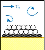
Traditional geometrical closed filters (figure 1-1) require construction of multiple layers of different diameter material (i.e. armour layer and one, or possibly several filter layers), such that it is impossible for the bed material to be transported, as the pores of the filter are too small (Verheij et al., 2010). The filter layer prevents transport of the bed material. The armour layer prevents erosion of filter material. However, the first difficulty with geometrical closed filters is the complex construction (and time-consuming) process of these multiple layers. The second difficulty is the likelihood of the loss of (fine filter layer) material by the local flow velocities during construction.

(10)

MSc thesis Page 10

Design guideline in the Netherlands

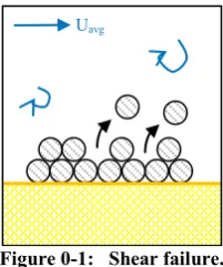
A summary of the general design guideline (Franken et al., 1995) for a geometrical open and closed filter in the Netherlands is visualized in figure 1-3. The main focus of this thesis is the step of determination of the interface stability. The first step is to determine design requirements and the hydrodynamic conditions in the outer flow. Next the type of protection is chosen, which in the context of this research is an geometrical open filter. The basic principle of designing a geometrical open filter is based on the consideration that the combination hydraulic load and duration does not exceed the design value for resistance or strength (CIRIA, CUR, CETMEF, 2007). Furthermore, the spatial extent of the protection is determined based on the scour area. Next, the top layer (which in single grading geometrical open filter is the same as the filter layer) is designed and it is checked whether it is stable for the given flow velocity and turbulence. External stability is defined as when the top layer grading is not mobile. This step is essential for the understanding of how a flow condition is incorporated in the design formulas for the required layer thickness. Shear failure is the failure mechanism that describes an undesirable situation of stones mobility (Chiew, 1995). The stable (nominal) grain size dn [m]is calculated with for example the widely applied formula of Shields for uniform

flow. This formula is rewritten (equation 1.1) with correction factors K [-] for specific non-uniform flow conditions (for horizontal bed) (Franken et al., 1995). K = 1 in uniform flow.

In equation 1.1., the grain size dn depends on the critical depth averaged flow velocity [m/s] the

correction factor of non-uniformity K (depends on the specific non-uniform flow condition), the critical mobility parameter ( 0.03 for initial phase of mobility and 0.055 for the phase of general transport of bed material), the density of the filter stone relative to the water density [-] and the roughness coefficient of Chezy C [m1/2 /s].

(1.1)

U0

[image:10.595.131.222.70.171.2]

U0

Figure 1-1: Geometrical closed filter. An armour layer covers the filter layer. Two grading system.

(11)

MSc thesis Page 11

Interface stability

The next step is assuring interface stability or stability of the bed material beneath the filter. If the designed layer dimensions are insufficient to prevent the bed material from transport through the pores, then the failure mechanism winnowing occurs (figure 1-5) (Chiew, 1995). If the geometrical open filter design is in agreement with the design requirements, than a preliminary design can be made (figure 1-3). In addition, shear failure, winnowing failure and 3 other failure mechanisms (not within the scope of this thesis) are described in appendix 1.

Figure 1-3: A modified version of guideline. Original is a guideline described by Rijkswaterstaat (Franken et al., 1995).

Determine spatial extent Design

requirements

Rough estimation of hydrodynamic conditions in the

outer flow.

Choice type of filter

Design top layer

Determine vertical layering [interface stability]

Check choice of protection

Preliminary design

In agreement with Design requirements

Not in agreement with Design requirements

Figure 1-4: Winnowing induced failure. The filter layer thickness is insufficient to damp the hydraulic load on the bed material. The underlying bed material is transported through the filter layer pores. This transport of bed material causes failure and filter layer settlement.

(12)

MSc thesis Page 12

Design formulas for interface stability

In order to assure interface stability in a geometrical open filter, several formulas were developed in the past (e.g. De Graauw et al., 1984, Klein Breteler in 1989 (Verheij et al., 2010), Wörman , 1989, Bakker et al., 1994 and Hoffmans, 2012).

A first approach calculates the filter grain size df15 (15% of the grading is smaller than the grain size df15)

for the filter layer-grading with a minimum layer thickness of two to three times the median grain size df50

in uniform flow (De Graauw et al., 1984, Klein Breteler in 1989 (Verheij et al., 2010), Bakker et al., 1994). If the filter layer-grading is insufficiently external stable, than a second (or more) filter-layer grading is designed on top of the first filter-layer-grading.

A second approach includes the layer thickness Df which results in a smaller number of

filter-layer-grading’s. The smaller number of filter-layer-gradings is more practical within the construction process. The focus is on the second approach. Two formulas for this second approach are the formula of Hoffmans (2012) and Wörman (1989). Hoffmans (2012) derived a formula on a theoretical basis that was validated with a limited number of tests. Wörman (1989) developed a formula based on experiments for non-uniform flow condition: flow with a cylindrical pier. Both the formula of Wörman and Hoffmans apply the design philosophy of simultaneous erosion of filter and bed material. The applicability of the formula of Hoffmans (2012) for both uniform flow (Van de Sande, 2012) and theoretically for non-uniform flow conditions (Hoffmans, 2012), is an advantage above other present design formulas and the main focus of this thesis. The formula of Wörman (1989) is based on experiments for the non-uniform flow, flow with a cylindrical pier. The formula of Wörman is also within the scope of this research as a reference formula for flow with a cylindrical pier. Figure 1-5 visualizes respectively the linear or logarithmic relation between the relative grain size df50/db50 and the relative layer thickness Df/df50 of the formula of Wörman and Hoffmans (2012).

Figure 1-5: The simplified version of the formula of Hoffmans (eq. 1.3 with )

(13)

MSc thesis Page 13

Design formula of Hoffmans (2012)

Hoffmans (2012) described two versions of the formula: (1) full version formula, (2) simplified formula. These full (equation 1.2) and simplified version (equation 1.3) include the suggested modifications by Van de Sande (2012) (change the relative layer thickness from to and a new version specific value for load damping coefficient (e.g. full version with simplified version with . Load damping coefficientαd is the parameter which describes turbulent kinetic energy damping by the filter.

The formula of Hoffmans (2012) relates the required layer thickness Df to the filter and bed material

characteristics and is valid for uniform flow conditions (Van de Sande, 2012). The design load conditions are indirectly incorporated in the median filter diameter df50, because the filter diameter is calculated with

for example equation 1.1 (e.g. and the flow velocity ū). In non-uniform flow conditions, e.g. additional turbulent conditions, the flow velocity and turbulence are indirectly incorporated in the larger required external stable filter grain diameter. A larger filter grain size df50 directly results in a larger relative layer

thickness (equation 1.2, 1.3 and figure 1-5).

(1.2) (1.3) Where:

Equation 1.3 is a rewritten after equation 1.2 with the assumptions (1 to 4) for the filter and bed characteristics.

The values for and are described by table 1-1. Within the formula, αd determines the

steepness of the curve (figure 1-5). The value for αd should be increased when the minimum filter layer

thickness is insufficient to prevent winnowing.

Hoffmans (2012) determined the value of αd based on damping of flow velocity fluctuations inside the filter

pores (use of data from Klar (2005). Van de Sande (2012) found a better fit with his test experiments and proposed a new αd,Sande (αd,Sande,safe) for both versions of the formula (equation 1.2 and 1.3).In addition, Van

de Sande proposed a αd for the lower limit of the band of simultaneous erosion of 0.28 for the full version

of the formula and 0.27 for the simplified version of the formula.

Table 1-1: values with additional safety for simplified version (s.v.) and full versions (f.v.) of the formula of

Hoffmans (2012).

Author [year] αd,f.v. [-] αd,s.v. [-]

Van der Sande [2012] 0.82 0.86

(14)

MSc thesis Page 14

Next to uniform flow conditions, in practice also locations of non-uniform flow can require scour protection (e.g. behind sluices, weirs, at bridge piers etc.). Figure 1-6 visualizes the flow conditions: (1) uniform flow, (2) flow with sill-induced turbulence and (3) flow with a cylindrical pier conditions. Flow condition (2) and (3) are conditions of non-uniform flow. Flow condition (1), (2) and (3) are often encountered as locations for which a geometrical open filter can be applied as a measure against scour. Conditions of uniform flow (1) are where the degree of turbulence and flow velocity profile are ‘uniform’ or normal in the flow direction, where bed level lowering is not desired. A condition of sill-induced additional turbulence (2) is where the fluctuations in the flow velocity are higher than uniform flow; also known as a backwards facing step. The local fluctuations induce an enhanced load (compared with uniform flow), where the highest load occurs near the reattachment point (red stones in figure 1-6). A cylindrical pier (e.g. bridge pier) (3) induces a three-dimensional flow field near the pier, which also enhances the local loads (Whitehouse, 1998).

Figure 1-6: Very schematic visualization of the unidirectionalflow conditions. Left image shows uniform flow. Middle

image shows additional turbulence (behind the reattachment point, at the red stones). Right image shows cylindrical pier (down flow and forward bound vortex), not shown is the enhanced flow near the pier due to flow contraction and the vortex shedding downstream of the pier. Chapter 2 describes the flow processes in more detail.

Hoffmans (2012) stated that the formula is theoretically valid for both uniform and non-uniform flow conditions. However, Hoffmans (2012) only described the validity for non-uniform flow conditions in a general way.

A first remark is that Van de Sande (2012) showed that flows with sill-induced additional turbulence increases bed mobility (test T06b) and flows with a rectangular or circular pier (T06c) also increases the bed mobility. Both tests were conducted with fixed filter material (glued). Increased turbulence levels induced by piers or sills on the flow also increase the filter mobility. Additional turbulence is already incorporated in the calculation of the df50 (equation 1.1, factor K), i.e. a larger filter grain size is calculated

and thus results in a larger relative layer thickness Df/df50 (equation 1.2, equation 1.3). The unknown filter

mobility in additional turbulent conditions is required to determine if the calculation of the larger filter grain size results in a sufficient relative layer thickness. Therefore, Van de Sande (2012) could not test the validity of αd,Sande in the formula of Hoffmans (2012) with his experiments for both type non-uniform flow.

A second remark is that, although it was not the primary purpose of her thesis, Van Velzen (2012) did test the validity of the formula of Hoffmans (2012) and Wörman (1989) for conditions with a cylindrical pier. Van Velzen (2012) applied two values of the relative layer thicknesses (3.7 [-] (marker L08) and 7.4 [-] (marker L01-L07)), classified only bed instability (winnowing/no winnowing) and applied a stable filter grain size to prevent shear failure. Results show an agreement between the data (marker L01-L07 and marker L08) and the formula of Hoffmans (2012) with αd,Hoffmans (figure 1-5) for non-disturbed depth

average flow velocities of ū = 0.34 m/s. Hence, data are also in agreement with the formula of Hoffmans (2012)and αd,Sande (Van de Sande, 2012) (appendix 2). However, at the moment only a single marker

(15)

MSc thesis Page 15

The formula of Hoffmans (2012) is not yet tested for conditions with sill-induced turbulence and confirmed with one single marker (and relative layer thickness). More tests are required to confirm the conclusion of data of Van Velzen (2012).

Design formula of Wörman (1989)

A comparable formula based on the same concept of simultaneous erosion which proved valid for cylindrical (bridge) piers is the formula of Wörman (1989). Within the context of this research of unknown validity of Hoffmans (2012) for piers, the formula of Wörman (1989) provides an interesting comparison. The Wörman formula relates filter, bed grain size and porosity linearly with the layer thickness Df, while

Hoffman’s formula relates the filter and bed characteristics to the layer thickness Df with a logarithmic

relation. Like the formula of Hoffmans (2012), load conditions (e.g. flow velocity) are incorporated in the filter grain size df50. Equation 1.4 describes the rewritten formula (Hoffmans, 2012) with the assumptions

of porosity = 0.4 [-], d85 = 1.25*d50 and d85 = (1/1.25) *d50.

(1.4)

Where:

The formula is explicitly described to be valid for 0<db85/df15<0.1 and test conditions similar to the test

conditions applied by Wörman (1989). It is derived from a stability criterion that includes the depth average flow velocity ū [m/s] for cylindrical piers. The derivation to the design formula includes the assumption that the local flow velocity u is two times the depth average flow velocity ū, which includes safety. Although Wörman (1989) describes the design formula does not include additional safety.

The test program consisted of depth average flow velocities of 0.22 < ū < 0.53 [m/s]. In addition, the water depth hw varied between 0.30 and 0.40 m and the tested layer thicknesses Df are between 10 and 100 mm.

The pier diameters applied are Dpier = 0.15 m and Dpier = 0.28 m.

New data

Recently, a database became available with experiments by Joustra (2012) conducted at the research institute Deltares. The database consists of water level, flow, filter surface height, filter pore-pressure measurements and camera images. The parameters layer thickness Df, grain size df50 and flow conditions

(16)

MSc thesis Page 16

1.2 Problem summary

The design formula for geometrical open filters of Hoffmans (2012) is not sufficiently validated for the non-uniform flow conditions: (1) sill-induced additional turbulence and (2) flow with a cylindrical pier. In addition, recently, a database became available with experiments performed by Joustra (2012), conducted at the research institute Deltares. The systematically varied flow conditions, layer thicknesses and filter grain sizes give the opportunity to validate the design formulas for uniform flow and non-uniform flow (e.g. sill induced additional turbulence or flow with a cylindrical pier).

The simplified and full versions of the formula of Hoffmans (2012) with respectively αd,Sande,s.v. = 0.86 and

αd,Sande,f.v = 0.82 are in of agreement with the uniform flow data of Van de Sande (2012) and e.g. Van

Huijstee & Verheij (1991) as described by Van de Sande (2012). Additional tests with uniform flow might support this previous validation result and would be useful because that would test the modification of αd

made by Van de Sande (2012).

In addition, the full and simplified versions of the formula with these αd’s are theoretically expected to be

in line with sill-induced additional turbulent conditions (e.g. downstream of a backwards facing step), because the layer thickness Df increases as a result of the increase of the filter diameter df50. At the moment

it is unknown if including additional turbulence within the calculation of df50 results in a sufficiently stable

relative layer thickness to prevent filter settlement (or the failure mechanism winnowing). However, first indicative measurements of sediment transport by Van de Sande (2012) show that the bed mobility is affected by the additional turbulent conditions (sill and pier induced). As the bed mobility increases due to the presence of a sill (Van de Sande, 2012), this could suggest that a higher αd for sill-induced additional

turbulence conditions should be applied.

Although Hoffmans (2012) suggests that the formula is valid for conditions of non-uniform flow, the results of comparison between data of Van Velzen(2012) and the formula are yet insufficient (one value relative layer thickness and relative grain size) to confirm the validity of the formula for flows with a cylindrical pier. Therefore, due to the limited data, additional validation for flows with a cylindrical pier is necessary to test the applicability of the formula for this type of non-uniform flow.

The Wörman (1989) formula is also based on simultaneous mobility of both geometrical open filter grains and bed grains, but this formula is based on tests with a cylindrical pier for flow conditions (0.22 < ū < 0.5m/s) and layer thickness Df between 1 and 10 cm. The formula is not yet tested for higher

(17)

MSc thesis Page 17

1.3 Research aim

The research aim of this thesis contributes to knowledge on how the minimum filter layer thickness required for a stable granular open filter is designed for uniform and non-uniform flows. The aim of this thesis is:

To test the validity of the design formula of Hoffmans (2012) for flows with sill-induced additional turbulence, and flows with a cylindrical pier and to test the validity of the design formula of Wörman (1989) for flow velocities over 0.5 m/s and filter layer thicknesses over 0.1 m at flows with cylindrical piers.

1.4 Research questions

The research aim is divided into 5 research questions. Research question 1-4 comes from the test of the validity of the design formula of Hoffmans (2012). More specifically, research question 1 follows from the availability of uniform flow data within the database. Research question 5 describes the test of validity of Wörman.

1) How do the data compare to previous validation of the load damping coefficient αd (Van de Sande,

2012) for uniform flow?

2) What is the effect of sill-induced additional turbulence on the load damping coefficient αd?

3) What is the effect of flows with a cylindrical pier on the load damping coefficient αd?

4) How do the data of flows with a cylindrical pier and flow velocities over 0.5 m/s compare to the design formula of Wörman (1989)?

5) How do the data compare to the previous validation of the formula of Hoffmans (2012) and the formula of Wörman (1989) based on data of Van Velzen (2012) for flows with a cylindrical pier?

Load damping coefficient αd is defined as αd,Sande,f.v. for the full version of the formula (equation 1.2) and

defined as αd,Sande,s.v. for the simplified version of the formula (equation 1.3). In addition, the data is defined

as the dataset of lab experiments conducted by Joustra (2012). The flow velocity is defined as the undisturbed depth average flow velocity ū [m/s].

1.5 Outline of thesis

(18)

MSc thesis Page 18

2 Theoretical framework

This chapter describes a brief summary of the theory about the flow processes relevant for the three research flow conditions (section 2.1), the theory about the incipient of motion and visual observation of mobility (section 2.2), and a more detailed description of the design formula of Hoffmans (2012) (section 2.3) and Wörman (1989) (section 2.4).

2.1 Flow mechanisms

Uniform and non-uniform flow

The mean and the fluctuating forces are both important in the mobility of the grains. The mean forces originate from the average shear stresses induced on the grains by the average flow velocities. Mclean et al., in 1994, Kleinhans & Van Rijn, in 2002 and Smeeckle & Nelson, in 2003 (Hofland, 2005) “ stated that: “Turbulence fluctuations of velocity and pressure are a key factor in the entrainment of bed material, as the mean forces alone are often not large enough to displace the particles”. The origin of the fluctuating forces can be the vortices shed from the stones upstream, the turbulence that originates from the difference in flow velocity in the outer flow or from the vortices that are shed from the stone itself, as suggested by Kalinkse in 1947 (Hofland, 2005). The velocity profile is logarithmic shaped and the theoretical magnitude of turbulence expressed as the depth average relative turbulence intensity r0 for uniform flow lies typically

between r0 = 0.042 [-] (for smooth, wide channels) and r0 = 0.126 [-] (for small rough channels) (Hoffmans,

2012).

Turbulence fluctuations can also be the result of a hydraulic structure, e.g. a backward facing step or a bridge pier. These latter conditions are classified as non-uniform flow, because there is a spatial variation in flow (e.g. water level, flow velocity and/or flow direction). The following sections describe the processes that are relevant for this thesis because the data of Joustra (2012) contains data of sill-induced additional turbulence and flows with a cylindrical pier.

‘Sill-induced additional turbulence’ or ‘backwards facing step’

The backward facing step is a classical situation of a condition with increased turbulent fluctuations. An example of the practical situation is an outflow structures (e.g. sluices, near power plants or at the Dutch Eastern Scheldt storm surge barrier). Figure 2-1 visualizes a sill (or backwards facing step) that influences the flow conditions behind a backwards facing step.

Behind the sill in the recirculation zone an eddy develops. Between the recirculation zone and the flow with higher flow velocities above the sill, a mixing layer develops where turbulence is generated. The upper flow reattaches at the reattachment point Xr and forms a new boundary layer. At the reattachment point, the

(19)

MSc thesis Page 19

velocities near the bed are nearly zero, but the damage to the unprotected bed is nearly maximal near the reattachment point (Hofland, 2005). This is because of the high levels of turbulence. In 1987 Nakagawa & Nezu (Hofland, 2005) found that the reattachment point is located further downstream for lower Reynolds numbers and for higher Froude numbers. Lower Reynolds numbers describe a less turbulent regime or more laminar flow regime. Higher Froude numbers are governed by increasing the depth average horizontal velocities or decreasing the water level) and describe a regime more towards supercritical flow. Schiereck (1995) described that the reattachment point is located at a distance downstream of 5-7 times the height of the sill. The location where the vertical and horizontal forces are strong enough for filter mobility is at the location between 10 and 20 times the height of the Sill according to Rajaratnam and Subramanya in 1968, Xingkui and Fontijn in 1992 and the experiments of Uwland in 1982 (Hoffmans, 2012). The flow recovers to the equilibrium conditions when the turbulent boundary layer thickness equals the water depth, and occurs after 20-50 times the water depth (Hoffmans, 2012).

Furthermore, the relative turbulent intensity r0 as function of x downstream of the sill (x>6*Dsill ) can be

calculated with the equation 2.1 as described by Hoffmans (2012):

(2.1)

Flow with a cylindrical pier

Another typical situation, next to uniform flow and the sill-induced additional turbulence is a condition with a cylindrical pier (e.g. bridge piers). Sumer and Fredsoe (2002) state the following relevant physical mechanisms (figure 2-2) that are responsible for scour near a pier; (1) Horse shoe vortices, (2) Lee wake vortices, (3) streamline contraction, (4) Down flow. The dominant feature in the scour process is the Horse shoe vortex (Breusers et al., 1977). Nielsen, Sumer, Fredsoe & Christensen (2010) observed that the hors-shoe vortex enters pores between the grains (figure 2-3) and suggest that this is the most important flow process regard to transport of sediment and sinking (i.e. bed instability) of the granular scour protection. In addition, Schiereck (1995) describes the down flow as a jet perpendicular to the surface of the granular material.

The flow field can be described as follows (figure 2-2 and figure 2-3): the approaching flow reaches the obstacle and an adverse pressure gradient develops at the upstream front of the pier due to the velocity gradient in the logarithmic vertical flow profile. The flow velocities are the highest near the surface and the lowest near the bed, due to friction. The flow decelerates the most at the surface level (high pressure at water surface, Bernoulli’s law) and decelerates less at the bottom (low pressure at bottom, Bernoulli’s law), both due to the presence of the pier in the flow. This vertical pressure difference causes a down flow to

Figure 2-2: Physical mechanism causing scour in the vicinity of an unprotected pier in steady current (Sumer

and Fredsoe, 2002).

(20)

MSc thesis Page 20

develop. As a result of the down flow and the strong adverse pressure gradient in the turbulent boundary layer, a forward bound vortex develops near the bed. The flow field near the side of the pier, forces the forward bound vortex to wrap around the pier, resulting in the horseshoe vortex. The forward bound vortex (located in front of the pier) and the horse shoe vortex (wrapping around the pier) are the most important mechanisms controlling scour of sediment around the base of the cylinder (Whitehouse,1998). Without a incoming boundary layer and a sufficiently strong adverse pressure gradient, the horse shoe vortex is not generated (Sumer and Fredsoe, 2002).

Lee wake vortices form behind the pier, when the pier boundary layer flow cannot follow the pier perimeter. Whitehouse (1998) describes: “The lee wake vortex is formed by rolling up and separation of the unstable shear layers generated around the structure and gives rise to eddies being shed downstream in a periodic fashion”. The formation of these eddies or lee wake vortices depends strongly on the pier Reynolds number ReD (2.2) and pier geometry. The pier Reynolds number is related to the non-disturbed

depth average velocity ū, Pier diameter D and viscosity v. Small Reynolds number result in no lee wake vortices (as the flow can follow the perimeter of the pier). If the ReD increases, lee wake vortices are

formed. When the ReD is sufficiently high, vortex shedding occurs (cut-off of lee wake vortices) (Sumer

and Fredsoe, 2002). Sumer and Fredsoe (2002) described equation 2.2:

(2.2)

The stream line contraction occurs due to the resistance caused by the obstacle and follows from the continuity restrictions. The same discharge passes a smaller area, so flow velocities must increase. This is visualized in small distances in the streamline at the side edges of the pier in figure 2-2 and figure 2-3.

2.2 Incipient motion

(Critical) Shields mobility parameter

According to the widely used sediment mobility theory of Shields(1936), the degree of sediment mobility depends on the shear stress, the difference in density between sediment and fluid, the particle diameter, the kinematic viscosity and the gravitational acceleration (Yang, 2003). When the shear stress τ (~related to u2) and the shield mobility parameter exceed the sediments critical value τc or c, the grains are transported.

The degree of transport under uniform flow is determined by the grain size specific c.

The stability of one grain diameter in a homogeneous bed under uniform flow conditions is characterized by the critical shield mobility parameter. In non-uniform flow, direction and magnitude of the flow differs from uniform flow. The effect of non-uniform flow can be incorporated in a in a factor K that is multiplied with the depth average flow velocity ucr (equation 1.1). Factor K is determined for specific condition and

will result in a higher or lower representative depth average flow velocity (Schiereck, 1995).

The shields shear stress theory is based on a homogeneous bed material. In practice both filter- and bed material are never completely uniform. In highly non-uniform grading (or wide grading) the processes of armoring can take place. The larger grains prevent the smaller grains from incipient of motion. Armoring increases strength of the bed material (Hoffmans,2012).

Visual observation of transport

Breusers (1977) described seven phases for visual observation of transport (Verheij et al., 2010). These classes are described by figure 2-4. Phase 6 describes the critical mobility as defined by Shields in 1936. Figure 2-4 therefore shows that transport of a grain can also occur locally below the critical value of mobility. For example, in general the filter grains of geometrical open filter have a diameter of df50 larger

than 2 mm (specific grain size D*>30) and c between than 0.030 (phase 1) and often 0.055 (phase 6).

According to Breusers (977), in that case phase 6 of permanent particle movement is observed at all locations. For engineering purposes, this is often not desirable. Therefore, c is chosen often equal to phase

(21)

MSc thesis Page 21

Figure 2-4: Seven phases of transport as described by Breusers in 1977 (Verheij et al., 2010) D* = d50(Δgrain*g/v^2).

2.3 Design formula of Hoffmans (2012)

Chapter 1 already described the simplified and full version of the formula. This sections describes theory behind the formula of Hoffmans (2012). The philosophy of simultaneous erosion is described by the characteristic relative strength [-]. For geometrical open filter this is incorporated within equation 2.3 (Bakker in 1994 and Grass in1970 (Hoffmans, 2012)). represents the mean characteristic strength of the base layer at the filter-bed interface. representsthe mean characteristic strength of the filter layer. The other parameters are described in section 1.1.

(2.3)

The load damping is not yet taken into account in equation 2.2. Hoffmans (2012) applied the turbulent kinetic energy coefficient kf (equation 2.4) as the measure for the damping of the loads in the geometrical

open filter.

(2.4)

The relative load at a certain depth in the filter is described by (equation 2.5). Hoffmans (2012) described that the relative load at the filter-bed interface is independent of the flow velocity as observations showed that kf (z) increases with increase in kb (equation 2.4). This means that the damping depth Ld only

depends on the load damping coefficient αd and the grain size df15. Thus in a general way, the increased

turbulence in the outer flow (i.e. sill-induced, pier induced) is theoretically incorporated into the formula of Hoffmans (2012). Hoffmans (2012) calibrated αd based on damping of flow fluctuations inside the filter

pores (figure 2.5). The velocity fluctuations were measured by Klar (2005) under uniform flow conditions. The relative load at the filter-bed interface is described by equation 2.6. z = 0 m is at the filter-outer flow interface and z = -Df is at the bed-filter interface.

(2.5)

(2.6)

(22)

MSc thesis Page 22

(equation 1.2). Change of Df/df15 to Df/df50 is based on a few wide filter grading experiments (Van de

Sande, 2012). However, at the moment the formula is not yet tested for non-uniform flow conditions. The non-uniform flow of a cylindrical pier is in a general way described by increased turbulence, but validation is recommended (Van de Sande, 2012, Hoffmans, 2012).

2.4 Design formula of Wörman (1989)

Wörman (1989) derived his formula (equation 2.8) based on a fitted empirical gradient (i.e. 0.16), Wörman (1989) stability criteria (equation 2.7), experiments with a cylindrical pier, the Isbash formula from 1935 (Breusers,1977) and a description for the local flow velocity of twice the depth average flow velocity (Worman, 1989) . Because the formula is based on piers, the horse shoe vortex is directly incorporated into the formula. In addition, Wörman (1989) stated that: “The governing dimensionless parameters describe suitable thickness of riprap layer, grain size of the riprap material, grain size of base material and mean flow velocity”. As described in section 1.1 the formula thus differs mainly from the formula of Hoffmans (2012) by the linear relation between these parameters and the thickness (Hoffmans ,2012). Hoffmans (2012) found a logarithmic relation. Explanation of parameters in equation 2.7 and 2.8 are described in section 1.1.

(2.7)

(2.8)

(23)

MSc thesis Page 23

3 Laboratory experiments

3.1 Test set-up

Laboratory experiments were part of the KPP (‘Kennis Primaire Processen’) research project and were executed between the 23rd of July and the 17th of August. The aim of the experiments was to populate a database for research into the relation between transport of bed material through the filter and into the flow, filter and bed characteristics for different flow conditions: these conditions being(1) uniform flow, (2) sill-induced additional turbulence and (3) conditions with a cylindrical pier. An additional aim was to populate the database with measurements of pressure signals and signal fluctuations within the filter. These pressure signals are outside the scope of this thesis.

The laboratory experiments are executed in the Atlantic Basin at Deltares. The set-up of the basin is visualized in figure 3-1 and 3-2.

Flow direction TEST SECTION 2

TEST SECTION 1

y-direction

x-direction

Sill (not during all tests)

Figure 3-1: Set-up of laboratory experiments in top view photo (left) and schematized view on the test sections (right). The blue arrows mark the flow direction. The striped area within the red lines shows the area where granular material covers the bed material. Only the red filled areas are the test sections.

TEST SECTION 1 TEST SECTION 2

(24)

MSc thesis Page 24

Test section 1 and test section 2

A part of the total Atlantic basin floor area is covered with concrete and a part is covered with fine sand (db50 = 0.165 mm). The basin in narrowed by construction of two walls. The (grey) zone of increased flow

velocities and contains sand is defined as ‘the testable area’ (shown in figure 3-2). The testable area has a length of 15 meters and width of 3 meters.

Within the testable area, two test sections are distinguished; (Test section 1; T1) flat bed, for conditions with and without additional turbulence, and (Test section 2: T2) flat bed with circular pier (Dpier = 0.15 m).

Test section 1 is used for two aims, that are achieved by application of two phases within the test series. Within the first phase, the damping of average velocity induced pressure and velocity fluctuation induced pressure within the filter is measured for different grain sizes and turbulent intensities. The second phase aims to measure the degree of filter settlement. The filter stones cover the bed material (sand, db50 = 0.16mm). The dimensions of this

test section (red in figure 3-1) are length L = 2.0m and width B = 2.0m. The thickness of filter layer was increased by keeping the filter top level equal to the surrounding area (figure 3-1), lowering the bed level (by removal of bed material) and filling this volume with filter material. Two type of flow conditions are tested in this test section: (1) uniform flow conditions and (2) additional turbulence flow. The additional turbulence is generated with a sill. Figure 3-3 visualizes the wooden sill and its location in front of test section 1. The wooden T-shaped sill with a height of 0.2 m (measured from the topside of the filter) is placed at 2.0 m in front of the pressure sensors.

A delineated (perimeter marked with red lines in figure 3-1) area is

designed in front of this test section. This area is defined as the ‘filter flow adaptation area’. The function is to provide an adaption length for infiltration of the flow into the filter layer. Here filter stones cover the bed

Figure 3-3: Wooden sill in front of test section 1.

TEST SECTION 2 TEST SECTION 1

Flow direction

y-direction

x-direction

Flow direction

- Sand grains - Filter grains - Geo-textile

- Sand interface (Tests S05-S06, U5-U11) - Sill (Tests: S01-S06)

- Concrete floor - Cylindrical pier

Figure 3-2: Top view and cross sectional view.

(25)

MSc thesis Page 25

material (sand). The dimensions are L = 3.5 m and B = 2.0 m. In addition, a slope (1:10) at a distance of 0.5 m of the left side of test section 1 is constructed in the preparation of some tests (U05-U11 and S05-S06). Test section 2 is used to measure the degree measure of filter settlement, down flow velocity and flow contraction effect on velocity at a cylindrical pier. The filter stones cover the bed material. The transparent pier has a diameter of Dpier = 0.15 m. The diameter of the test section 2 is approximately Ct2 ≈ 0.83m. This

corresponds to the representative bed protection Ct2≈6*D by Whitehouse (1998). The thickness of the filter

layer was increased by keeping the filter top level equal to the surrounding area (figure 3-2), lowering the bed level (by removal of bed material) and filling this volume with filter material.

The remaining area surrounding both test sections (gray in figure 3-1) contains bed material covered with geo-textile. The geo-textile is covered with stones of similar size as the test sections to fixate the location of the geo-textile. Geo-textile prevents having to reconstruct the filter top layer surrounding the test sections after each test.

Test parameters

The flow conditions only contain a current (no waves). The parameters that are varied during the test program are the layer thickness Df, [mm], filter grain size df50 [mm], average flow velocity ū [m/s] and flow

conditions consisting of (1) uniform flow, (2) additional turbulence and (3) with cylindrical pier. The three flow velocities that were tested are; 0.5 m/s, 1.0 m/s and 1.5 m/s. The water level was kept at 1.0 m for

ū = 0.5 m/s and ū = 1.0 m/s. To achieve the average flow velocity 1.5 m/s, water levels were decreased to hw = 0.67 m, because of limited discharge capacity. The test duration was 1.5 hours per test.

Two filter gradations are tested. The first gradation has a median filter diameter df50 = 27.0 mm, the second

a filter diameter of df50 = 20.0 mm. The associated relative grain size diameter (df50/db50) is respectively 146

[-] and 109 [-]. The first filter grain diameter has a df15= 22 mm and df85 = 40 mm. The second filter grain

diameter has a df15 = 16 mm and df85 = 22mm. The open filter grain diameters are selected to be ‘just’

external stable with phase 1 ( c = 0.03) using equation 1.1 (Schiereck, 1995). The sieve curves are

described by appendix 3 and 4. The test parameters per test are described in section 3.2 Test program.

3.2 Test program

Table 3-1 describes the test program and the values for each test parameter during the test. The ID of the database, or Test ID (e.g. 1a) is redefined in this thesis to the Report ID to distinguish the flow conditions and the flow velocity. The ID stands for the (Report or Test) number. The U, S and P in front of the number represent respectively flow condition uniform flow, sill-induced additional turbulence and cylindrical pier. Furthermore, table 3-1 contains the absolute filter layer thickness Df, filter and bed material grain sizes

(both absolute and relative) and the degree of wide-grading by Vg. Data of the density of the bed and filter

material is not available, therefore the density of both filter and bed material is assumed 2650 kg/m3. A coupled test is for example test T01 (‘T01a+T01b’), or an uneven Report ID combined with the following ‘even’ number. The flow velocity is increased from T01a to T01b.

(26)

MSc thesis Page 26

Table 3-1: Overview of test parameters. The colours green, orange and blue represent the flow conditions uniform

flow, flow with sill-induced additional turbulence and flows with a cylindrical pier, respectively. Ū = U0. Hw = 1.0 m

(27)

MSc thesis Page 27

3.3 Data

The main data resource for this thesis is a database which resulted from laboratory experiments carried out as part of the KPP research project (‘Kennis Primaire Projecten’) of Deltares and Rijkswaterstaat (Joustra, 2012). At the start of this research, the database consisted only of un-processed raw data. Section 3.3.1 describes the available data, while section 3.3.2 describes the data processing. Furthermore, validation results as interpreted by Van de Sande (2012) are added to this thesis as a reference. This validation results are based on data of Van Huijstee & Verheij (1991), Bakker in 1960 (Van de Sande, 2012), Van der Sande (2012), Van Velzen (2012) and Wörman (1989). Appendix 2 describes these validation results.

3.3.1 Raw dataset

Four types of data are obtained by the tests: (1) sub-water surface camera images, (2) hydrodynamic data, (3) bathymetry data and (4) pressure data inside the filter layer. The focus of this research is on data types (1), (2) and (3). (4) was recorded in anticipation of further research.

Submerged camera images were made during the tests at test section 1 (position near the wall) and test section 2 (position inside pier).

Furthermore, six EMS flow velocity meters measured the flow velocity in two directions. During the test, four flow sensors measured the flow velocity in the horizontal plane (x- and y-direction) along the width in front of the test sections. These four EMS meters where relocated occasionally (both vertical as horizontal), to measure 1 minute flow velocities at multiple x- and z-positions within the testable area. Furthermore, two additional EMS measured the flow velocities near the cylindrical pier. One EMS measured the vertical and horizontal flow (x- and z- direction) in front of the pier and one EMS measured the horizontal flow at the side of the pier. Also, the water level is measured at the x - location of the pressure sensors (test section 1), near the side-walls.

The bathymetry data consists of raw 3D -stereo-photography (3D-SP) coupled-images and internal camera images. 3D-SP is applied before and after each ‘coupled test’ (e.g. test ID ‘T01’). Processing the 3D-SP data results in spatial information (x, y, z) of the filter-outer flow interface on the time step before and after the coupled test. The bathymetry by 3D-SP is available for before test U5, U7, U9, S5, P1, P3, P5, P7, P9, P11, P13 and P15. In addition, the bathymetry data by 3D-SP is available after test U6, U8, U10, S6, P2, P4, P6, P8, P10, P12, P14 and P16. No 3DSP data is available for test U1, U2, U3, U4, S1, S2, S3 and S4. The bathymetry data by internal camera imagery is available for before, after and during tests P1 to P17, but outside the scope of this thesis.

3.3.2 Data processing

The raw data (underwater camera images, 3DSP) as described in section 3.3.1 must be processed, before the data can be applied in the validation of the design formulas. In addition, the flow velocity measurements are processed to describe the flow conditions during the tests (e.g. with flow velocity and turbulent intensity profiles, etc.).

Visual observation to classify filter and bed stability

(28)

MSc thesis Page 28

Verification of filter instability in uniform flow and flows with sill-induced additional turbulence The method 3D Stereo-Photography (3D-SP) is applied to quantify the degree of filter settlement for the conditions of uniform flow and sill-induced additional turbulence. First, the method 3D-SP is used to calculate the bathymetry from a set of photo-pairs made before and after each ‘coupled test’. Within the 3DSP method, the degree of disparity between two photos (photo pairs) is used as input for the calculation of the filter-outer flow interface level. The larger the distance between a pixel in photo 1 and the same pixel in photo 2, the closer this pixel (point) is to the camera. This is the same principle as two eyes estimating distance. The photo pairs are made at multiple locations around the test section. The data set of photo pairs is the input for the calculation and reconstruction of the bathymetry. Next, the difference in filter-outer flow interface is computed by subtraction of the initial bathymetry from the final bathymetry. A negative value describes a decrease, and could either describe filter settlement (i.e. bed instability), filter instability or both. The filter-outer flow interfaces levels and differences are calculated with Matlab-scripts available at Deltares. The method of stereo-photography is commonly used in consultancy studies at Deltares. The resolution of the grid is 1mm and typical measurement errors in perfect conditions are in the order of 1 mm. Figure 3-6 and figure 3-7 show the equipment of stereo-photography.

(29)

MSc thesis Page 29

Figure 3-4: One frame of the video of camera 1. Camera 1 filmed the condition uniform flow and the condition sill-induced additional turbulence. The flow direction is from left to

right.

Figure 3-5: One frame of the video of camera 2. Camera 2 filmed the condition with a cylindrical pier. The camera is fixed inside pier, facing downwards. The red filter stones are on top of the white-grey bed material. Flow direction is from left to right.

(30)

MSc thesis Page 30

Figure 3-7: Stereo photography set. The set contains the camera attached to a laptop (on the table), the markers (around pile) and baseplate (attached to wall).

(31)

MSc thesis Page 31

Flow conditions uniform flow and flows with sill-induced additional turbulence

The flow profiles (u(x, z)) and turbulent fluctuations profiles (as described by the root-mean-square values RMS (equation 3.1) and the relative turbulent intensities ru (equation 3.2)) are calculated from the EMS

flow velocity data measured at the test section with uniform flow and near the test section with sill-induced additional turbulence. These profiles describe the flow conditions (uniform flow and flows with sill-induced additional turbulence).

The sill in front of the test section is expected to induce additional turbulence in the test section. The increase in turbulence intensity increases the degree of mobility of the filter stones (Schiereck, 1995) and it is expected (based on observations of Van de Sande (2012)) that an increase in turbulent fluctuations increases the degree of bed instability.

Statistics (median u, root-mean-squared (RMS) and relative turbulence intensity ru) are calculated from the

flow velocity data measured at multiple depths downstream of the locations of the sill for the conditions uniform flow and flows with sill-induced additional turbulence, to quantify the effect of the sill on the flow and the investigate the distribution of these statistics over the width of the test section. The location of the flow- , turbulence profiles and EMS are show in figure 3-9 (top view). The cross sections where the flow profiles are measured are visualized by figure 3-11 and 3-12. The data processing software Matlab is used to calculate and visualize the statistics into figures.

Flow condition with a cylindrical pier

Next, the vertical and horizontal velocity raw signals measured in front of the cylindrical pier are processed. This provides insight in occurrence and magnitude of the expected down flow and/or horse shoe vortex in front of the pier. The cross section at test section 2 (with a cylindrical pier) is visualized by figure 3-10.

The median and RMS values calculated from the vertical flow velocity signal describe the degree of the down flow and down flow fluctuations. The statistics are calculated for test P15, P16 and P17 with flow velocities of respectively ū = 0.5 m/s, ū = 1.0 m/s and ū = 1.5 m/s. Test P15, P16 and P17 all have the same relative layer thickness and relative grain size. In addition, these test also have relative no to minor degree of filter-outer flow interface decrease. The statistics are calculated over a 10 minutes time window. The data contains a gradually increasing flow velocity during test P17 between t = min and t ≈ 35 min, therefore with a additional buffer of 8 minutes the time window is chosen to be from 41 to 51 minutes.

_(3.1)

(32)

MSc thesis Page 32

Camera (C1)

Flow direction Flow

direction

x = +8m

x = +4m x = +11m

y-direction

x-direction

Internal camera (C2)

Figure 3-9: Location of flow velocity profile measurements; x = 4 m, x = 8 m and x = 11 m. The distance is described in mm.

Undisturbed flow direction u0

EMS 5 EMS 6

hEMS5-6 ≈ 12.5 cm Distance to pier, EMS5-6≈5 cm

Figure 3-10: Location of EMS 5 and 6 relative to the pier. Right image shows the cross-sectional view of the Pier.

EMS 4 EMS 3 EMS 2 EMS 1

Z=1.0m Z=0.5m Z=0.4m Z=0.0m Z≈-0.05m Y=0.0m Y=1.0m Y=2.0m

Y=3.0m Y=2.6 m Y=2.5 m Y=1.9 m Y=1.1 m Y=0.5 mY=0.4m

Y-direction [m]

Figure 3-11: The default position and lateral cross-section of the EMS sensors at location x = 4 m. This also visualizes the cross-section at location x = 11 m.

EMS 4 EMS 3 EMS 2 EMS 1

Z-direction [m]

Z=1.0m

Z=0.5m

Z=0.4m

Z=0.0m

Z≈-0.05m Z=-0.20m

Y=0.0m Y=1.0m

Y=2.0m

Y=3.0m Y=2.6 mY=2.5 m Y=1.9 m Y=1.1 m Y=0.5 mY=0.4m Y-direction [m]

Figure 3-12: Lateral cross-section at x = +8 m for test U1-U4 and S1 and S2. Layer thickness was modified for the other tests. The layer thickness during test U5