An Application of Non–Linear Cobb Douglas Production Function to Selected Manufacturing Industries in Bangladesh

(1)

An Application of Non-Linear Cobb-Douglas Production

Function to Selected Manufacturing Industries in

Bangladesh

Md. Moyazzem Hossain1, Ajit Kumar Majumder2, Tapati Basak2 1

Department of Statistics, Islamic University, Kushtia, Bangladesh 2

Department of Statistics, Jahangirnagar University, Dhaka, Bangladesh Email: [email protected], [email protected], [email protected]

Received May 14,2012; revised June 20, 2012; accepted July 2, 2012

ABSTRACT

Recently, businessmen as well as industrialists are very much concerned about the theory of firm in order to make cor- rect decisions regarding what items, how much and how to produce them. All these decisions are directly related with the cost considerations and market situations where the firm is to be operated. In this regard, this paper should be help- ful in suggesting the most suitable functional form of production process for the major manufacturing industries in Bangladesh. This paper considers Cobb-Douglas (C-D) production function with additive error and multiplicative error term. The main purpose of this paper is to select the appropriate Cobb-Douglas production model for measuring the production process of some selected manufacturing industries in Bangladesh. We use different model selection criteria to compare the Cobb-Douglas production function with additive error term to Cobb-Douglas production function with multiplicative error term. Finally, we estimate the parameters of the production function by using optimization subroutine.

Keywords: Cobb-Douglas Production Function; Newton-Raphson Method; Manufacturing Industry; Bangladesh

1. Introduction

A developing country like Bangladesh which is facing enormous problems so far as industrialization policy is concerned does not follow the policy of Marxian Economy, neither thus it strictly follow the policy of a Capitalist country. The economy of Bangladesh actually turned out to be a mixed economy since a long time. The industry sector was severely damaged during the war of liberation in 1971. After a series of adjustments and temporary changes in state policy, the government finally adopted a new industrial policy in 1982. Every industrialist tries to produce goods with maximum profit but with minimum cost. In order to do this, it has to be decided what to produce, how much to produce and how to produce. The industries need various inputs such as labor, raw material, machines etc. to produces goods. An industry’s production cost depends on the quantities of inputs it buy and on the prices of each input. Thus an industry needs to select the optimal combination of inputs, that is, the combination that enables it to produce the desired level of output with minimum cost and hence with maximum profitability. So the main objective of this paper is to select the appropriate Cobb-Douglas production function. We use different model

selection criteria to compare the Cobb-Douglas production function with additive error term to Cobb-Douglas production function with multiplicative error term. Finally, we estimate the parameters of the production function by using optimization subroutine.

2. Cobb-Douglas Production Function

The Cobb-Douglas production function is the widely used function in Econometrics. A famous case is the well- known Cobb-Douglas production function introduced by Charles W. Cobb and Paul H. Douglas, although antici- pated by Knut Wicksell and, some have argued, J. H. Von Thünen [1]. They have estimated it after studying different industries in the world, for this it is used as a fairly universal law of production.

The Cobb-Douglas production function with multiplicative error term can be represented as,

3 2 1

t t t t

p L K u 

t

p L

(2.1)

where, is the output at time t; t is the Labor

input; Kt is the Capital input; 1 is a constant; t is

the random error term.

u

2

 and 3 are positive pa-

(2)

The Cobb-Douglas production function with additive error term can be represented as,

3 2

t t t t

p  L K  u

t

p L

1

 (2.2)

where, is the output at time t; t is the Labor

input; Kt is the Capital input; 1 is a constant; t is

the random error term.

u

2

 and 3 are positive pa-

rameters.

3. Literature Review

Production functions for the industrial sector as a whole as well as for seven important industries in India are worked out based on cross-section data relating to indi- vidual firms for the two years 1951 and 1952 (V. N. Murti and V. K. Sastry) [2]. De-Min Wu [3], derives the exact distribution of the indirect least squares estimator of the coefficients of the Cobb-Douglas production function within the context of a stochastic production model of Marschak-Andrews type. The stochastic term in Cobb- Douglas type models is either specified to be additive or multiplicative (Stephen M. Goldfeld and Richard E. Quandt) [4]. They developed a model in which a Cobb- Douglas type function is coupled with simultaneous multiplicative and additive errors. This specification is a natural generalization of the “pure” models in which either additive or multiplicative stochastic terms are introduced. A Cobb-Douglas type function with both multiplicative and additive errors has been proposed by Gold- feld and Quandt [5]. They suggested a maximum likely- hood approach to the estimation of a Cobb-Douglas type model when the model includes both multiplicative and additive disturbance terms. As expected, an analytical expression for the solution to the maximization problem did not exist. Indeed, because of the complexity of the likelihood function, their maximization algorithm had to be used in conjunction with a numerical integration technique.

Kelejian [6] generalize and simplify the work by Goldfeld and Quandt [5]. Specifically, an estimation technique is suggested which does not require the specification of the disturbance terms beyond their means and variances, which does not require the compounding of a maximization algorithm with a numerical integration technique, but yet leads to asymptotically efficient estimates of the parameters of the regression function. In addition, the procedure readily lends itself to interpreta- tion. For instance, it will become evident that if the distribution of the multiplicative disturbance term is not known, the scale parameter of the model (unlike the other parameters) will not be identified. The origins of the Cobb-Douglas form date back to the seminal work of Cobb and Douglas [1], who used data for the US manufacturing sector for 1899-1922 (although, as Brown [7]),

Sandelin [8], and Samuelson [9], indicate, Wicksell should have taken the credit for its “discovery”, for he had been working with this form in the 19th century).

Cheema [10], Kemal [11], and Wizarat [12], showed the performance of large-scale manufacturing sector of Pakistan. Moreover tax holidays also encourage investment in the industrial sector. For example, Azhar and Sharif [13], and Bond [14], empirically proved the positive correlation between tax holidays and industrial output. But it is also worth to note that tax rate and output of manufacturing sector are inversely related. The authors used the data of West Virginia State of United States. However, Radhu [15], showed the positive correlation between indirect tax rates and prices of the commodities. Vijay K. Bhasin and Vijay K. Seth [16], estimate production functions for Indian manufacturing industries and to find whether plausible and meaningful estimates can be obtained for returns to scale, substitution, distribution, and efficiency parameters. Some studies are based on data collected through surveys specially designed for estimate the levels of technical efficiency (TE) (e.g., Lit- tle et al., [17], Page [18]). Many of the studies are concerned with estimating and explaining variations in TE only in Small-Scale Industrial Units by fitting either a deterministic or a stochastic production frontier (e.g., Bhavani [19], Goldar [20], Neogi and Ghosh [21], Ni- kaido [22]). A review of other studies in this area may be found in Goldar [23].

All these studies, however, use data relating to years prior to the economic reforms. For instance, Bhavani [19] uses data collected under the first Census of small scale industrial units in 1973 to estimate the TE of firms at the 4-digit level industries of metal product groups by fitting a deterministic translog production frontier with three inputs-capital, labor and materials- and observes a very level of average efficiency across the four groups. Simi- larly, on the basis of the data made available by the Sec- ond All India Census of Small Scale Industrial Units in 1987-1988, Nikaido [22] fits a single stochastic production frontier, considering firms under all the 2-digit industry groups and using intercept dummies to distinguish different industry groups. He finds little variation in TEs across industry groups and a high level of average TE in each industry groups. Neogi and Ghosh [21] examine the inetrtemporal movement of TE using panel industry-level summary data for the years 1974-1975 to 1987-1988 and observe TEs to be falling over time.

(3)

ductivity in Canada (M. Daly, Gorman, Lenjosek, MacNevin, & Phiriyapreunt [25]), productivity and imperfect competition in Italian firms (Contini, Revelli, & Cuneo [26]), explaining total factor productivity differentials in urban manufacturing of US (Mullen & Wil- liams, [27]). Total factor productivity growth in manufacturing has been examined by applied parametric and non-parametric approaches. In most of the studies have used non-parametric approach, wherein total factor productivity growth has decomposed into efficiency change and technological change. Efficiency change measures “catching-up” to the isoquant while technological change measures shifts in the isoquant. For example, see Weber and Domazlicky [28]; Nemoto and Goto [29]; (Maniada- kis and Thanassoulis [30] and Radam [31].

The studies by Golder et al. [32], Lall and Rodrigo

[33], and Mukherjee and Ray [34], however, relate to the post-reform era. Using panel data for 63 firms in the engineering industry from 1990-1991 to 1999-2000 drawn from the Prowess database (version 2001) of the

Centre for Monitoring Indian Economy, Goldar et al.

[32] fit a translog stochastic production frontier to estimate firm-level TE scores in each year. They find the mean TE of foreign firms to be higher than that of do- mestically owned firms but do not find any statistically significant variation in mean TE across public and pri- vate sector firms among the latter group. They can at- tempt to explain variation in TEs in terms of economic variables, including export and import intensity and the degree of vertical nitration. Lall and Rodrigo [33] examine TE variation across four industrial sectors in In- dia during 1994 and consider TE in relation to scale, location extent of infrastructure investment and other determinants.

Md. Zakir Hossain, M. Ishaq Bhatti, Md. Zulficar Ali, [35], reviews some models recently used in the literature and selects the most suitable one for measuring the production process of 21 major manufacturing industries in Bangladesh. In particular, they estimates and tests the coefficients of the production inputs for each of the selected manufacturing industries using Bangladesh Bureau of Statistics annual data over the period 1982-1983 through 1991-1992. Cheng-Ping Lin [36] analyzes the cost function of construction firms with due considera- tion of their available resources by using Cobb-Douglas

Production and Cost Functions. Moosup Jung, et al. [37]

made a study on Total Factor Productivity of Korean Firms and Catching up with the Japanese Firms. They measured and compared the TFP of both Korean and Japanese listed firms of 1984 to 2004. They found that the average TFP of Korean firms grew about 44.1% between 1984 and 2005, with 2.1% annual growth rates. Industry was observed to be outstanding.

Danish A. Hashim [38] made research on “Cost and

Productivity in Indian Textiles” for Indian Council for Research on International Economic Relations. His observations and findings are: there is an inverse relation- ship between the unit cost and productivity: Industry and States, which witnessed higher productivity (growth) experienced lower unit cost (growth) and vice-versa. Better capacity utilization, reductions in Nominal Rate of Protection and increased availability of electricity are found to be favorably affecting the productivity in all the three industries. M. Z. Hossain and K. S. Al-Amri, [39] find that for most of the selected industries the C-D function fits the data very well in terms of labor and capital elasticity, return to scale measurements, standard errors,

economy of the industries, high value of R2 and rea-

sonably good Durbin-Watson statistics. The estimated results suggest that the manufacturing industries of Oman generally seem to indicate the case of increasing return to scale. Of the nine industries, seven exhibit increasing return to scale and only the rest two show decreasing return to scale. They also find that no industry with constant return to scale.

4. Estimation Procedure

Equation (2.1) is nearly always treated as a linear rela- tionship by making a logarithmic transformation, which yields:

1 2 3

logp_t log  logL_t logK_tlogu_t

logu

1 log

(3.1)

where, is treated as an additive random error with

a zero mean. In this form the function is a single equation

which is linear in the unknown parameters:  , 2

and 3.

In the case of Equation (2.2), the minimization of,

2

u



is no longer a simple linear estimation problem.

To estimate the production function we need to know different types of non-linear estimation. In non-linear model it is not possible to give a closed form expression

for the estimates as a function of the sample values, i.e.,

the likelihood function or sum of squares cannot be transformed so that the normal equations are linear. The idea of using estimates that minimize the sum squared errors is a data-analytic idea, not a statistical idea; it does not depend on the statistical properties of the observations. Newton-Raphson method is one of the method which are used to estimate the parameters in non-linear system.

4.1. Newton-Raphson Method

Newton-Raphson is one of the popular Gradient methods of estimation. In Newton-Raphson method we find the

values of j that maximize a twice differentiable con-

(4)

 

g t

 

thod we approximate  at  by Taylor series

expansion up to the quadratic terms

 

   







1 2 t t g g

 



t

t t t

              _ G H  

where,

 

t i g t    G    _ 

  is the gradient vector and

 

2

t i k g t    H      _{ }   

 

g

is the Hessian matrix. This Hes-

sian matrix is positive definite, the maximum of the ap-

proximation  occurs when its derivative is zero.

   

t t

 

  

G H





 

1

 

0 t t          

H  G

1 t

(3.11)

This gives us a way to compute  

 

1

 

t t

, the next value in iterations is,

1

t t

  _ __  _ _

H  G

The iteration procedures continue until convergence is achieved. Near the maximum the rate of convergence is quadratic as define by

2 ˆ ˆ t t i i c 1 i i      0 

for some c when it is near ˆi for all . Thus

we get estimates

i

ˆ

i

 by Newton-Raphson methods.

For the model (2.2), to estimate the parameters we minimize the following error sum squares

 

1 n t S p 



2 3



2 1

t L Kt t

 

  

In case of nonlinear estimation we use the score vector and Hessian matrix. The elements of score vector are given below:

 

_

_

1 1 1 2 * n t t t S

p L K



 



  





2 t3 *



L Kt2 t3



 

 

 

 



2 3





 



2

1 1

2 * * ln *

n

t t t t

t

S

p L K  L

      

 



_ 



2 3



1L Kt t

 

 



 



2 3





 



3

1 1

2 * * ln *

n

t t t t

t

S

p L K  K

      

 



_ 



2 3



1L Kt t

 

 



Also the elements of Hessian matrix are given below:



2 3



2 2 2 1 1 2 * n t t t S

L K 

     



 

_

_{ }

_

_

_{ }

_











 







3 3 2 2 3 3 2 2 2 1 1 1 2 1

2 * ln * *

* ln *

n

t t t t t

t

t t t t t t

S

L L K L K

p L K L L K

               _  _      _



 

_

_{ }

_

_

_{ }

_







 











3 3 2 2 3 3 2 2 2 1 1 1 3 1

2 * ln * *

* ln *

n

t t t t t

t

t t t t t t

S

K L K L K

p L K K L K

               _  _      _



 

_

_{ }

_

_

_







 











3 2 3 3 2 2 2 2 1 2 1 2 2 1 1

2 * ln *

* ln *

n

t t t

t

t t t t t t

S

L L K

p L K L L K

             _  _     



 











 

















 





 











3 3 2 2 3 3 2 2 2 2 3 1 1 1 1 1

2 * ln * * ln *

* ln * ln *

n

t t t t t t

t

t t t t t t t

S

K L K L L K

p L K K L L K

                     _    _



 

_

_{ }

_

_

_







 











3 2 3 3 2 2 2 2 1 2 1 3 2 1 1

2 * ln *

* ln *

n

t t t

t

t t t t t t

S

K L K

p L K K L K

             _       _



 

Hence the Score vector is

 

1 2 3

, ,

S  S  S 

            _ _ _    G

 

and Hessian matrix is

 



 

2 2 2

2

1 2 1 3

1

2 2 2

2

1 2 2 2 3

2 2 2

2

1 3 2 3 3

S S S

        _ _{ } _{ }         _ _ _ _ _ _{ }                               _{ } _{ } _    H

model. Some of these criteria are discuss below.

4.2. Model Selection Criteria

(5)

4.2.1. Finite Prediction Error (FPE)

Akaike (1970) developed Finite Prediction Error proce- istic of this procedure, which is known as FPE. The stat

dure can be represented as,

FPE ESS T K

T T



 

 _ _{ }_ _K

where, T is the number of observations and K is the

number of estimated parameter (R anathan [40]).

Akaike (1974) also developed another procedure which The form of am

4.2.2. Akaike Information Criteria (AIC)

is known as Akaike Information Criteria. this statistic is given below,

2

AIC e

K T

T

  

 

n me variables are dropped (Ramanathan [40]).

Q) Criterion

Hunnan and Quinn (1979) developed a procedure which is procedure

ESS  

 

 

The value of AIC deceases whe so

4.2.3. Hunnan and Quinn (H

is known as HQ criteria. The statistic of th can be represented as





2 

HQESS lnT k T T

 

 

The value of HQ will decrease provided there are at observations (Ramanathan [40]).

Craven and Wahba (1978) developed a procedure which



C criteria. The form of

least 16

4.2.4. SCHWARZ Criterion

is known as SCHWARZ BI



this procedure is represented as

SCHWARZ E S K T

 _ S _T

T 

also decrease provided there are at least 8 observations (Ramanathan [40]).

Craven and Wahba (1981) developed a procedure which teria. The form of this pro- The value of SCHWARZ will

4.2.5. SHIBATA Criterion

is known as SHIBATA cri

cedure is represented as

2 SHIBATAESS T  K

T T

 

  .

When some variables dropped SHIBATA will increase

(Ramanathan [40]

ross Validation (GCV)

Generalized Cross Validation (GCV) is another proce- (1979). ).

4.2.6. Generalized C

dure which is developed by Craven and Wahba The form of the statistic is given below

2

GCV ESS 1 K

T T



 

   

_ __ _{ }_

   

If one or more variables are dropped t en GCV will decrease (Ramanathan [40]).

The model selection criteria Rice developed by Craven e form of this criterion can be rep-

h

4.2.7. Rice Criterion

and Wahba (1984). Th resented as

1 2

ESS  K 

RICE 1

T T

   

_ __ _ __

    .

(Ramanathan [40]).

iterion

The form of this criterion can be represented as

4.2.8. SGMASQ Cr

1

SGMASQ ESS 1 K



 

   

_ __ _{ }_ .

T T

   

If SGMASQ decreases (that is R2 inc ses) when

one or more variable dropped, then GCV and RICE

will also decreas ).

stries of

Bangladesh for This Study

ang-

lad ladesh Census of

Leather Products; r;

s (Wooden);

;

cts; Industries;

s;

6.

In case of Cobb-Douglas production function with multi- rea

es (Ramanathan [40]

5. Selected Manufacturing Indu

In recent publications of “Statistical Yearbook of B esh [41]” and “Report on Bang

Manufacturing Industries (CMI) [42]” published by BBS, we get the published secondary data for the major manufacturing industries of Bangladesh over the period 1978- 2002. We have chosen the following manufacturing industries for the ongoing analysis.

1) Manufacturing of Textile; 2) Manufacturing of Leather & 3) Manufacturing of Leather Footwea 4) Manufacturing of Wood & Cork Products; 5) Manufacturing of Furniture & Fixture 6) Manufacturing of Paper & Paper Products; 7) Manufacturing of Printing & Publications; 8) Manufacturing of Drugs & Pharmaceuticals 9) Manufacturing of Industrial Chemical; 10) Manufacturing of Plastic Products; 11) Manufacturing of Glass & Glass Produ 12) Manufacturing of Iron & Steel Basic 13) Manufacturing of Fabricated Metal Product 14) Manufacturing of Transport Equipment; 15) Manufacturing of Beverage;

16) Manufacturing of Tobacco.

(6)

Con

HQ WA

plicative error terms i.e., for intrinsically linear model

and additive errors i.e., for intrinsically nonlinear model,

we get the following estimates by using different model selection criteria discussed in Section 4.2.

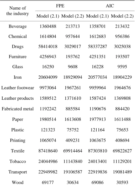
From Table 1, we observe that, the Cobb-Douglas

production function with additive error (2.2) performs

better fo the selected manufacturing industries based on r

the data under study period. Thus the strictly nonlinear models (which are nonlinear with additive error terms) seem to be better than intrinsically linear model (which are nonlinear with multiplicative error terms).

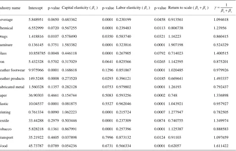
Now we estimate the parameters of the Cobb-Douglas production function with additive errors by using op-

timization subroutine. The estimates are given in Table

2.

There are economies of scale in the manufacturing of Drugs & pharmaceuticals, Furniture & fixtures (wooden), Iron & steel basic, Leather footwear, Fabricated metal products, Plastic products, Printing & publica-

tions, Tobacco since  1 for these industries. There

are diseconomies of scale in the Beverage, Chemical, Glass & glass products, Leather & leather products, Paper & paper products, Textile, Wood & crock prod-

ucts industries, Transport equipment since  1 for

[image:6.595.59.286.419.734.2]

these industries.

Table 1. Values of different model selection criter two models under stud

ia of y.

FPE AIC Name of

the industry

Model (2.1) Model (2.2) Model (2.1) Model (2.2) Beverage 1360488 213713 1358701 213432 Chemical

1 1

Leath ear 9 1 1

Leather

Pr

8 6 6

1 1

T

1614804 957644 1612683 956386

Drugs 58414018 3029017 58337287 3025038

Furniture 4256943 193762 4251351 193507

Glass 16250 9608 16228 9595

Iron 20604099 8929094 20577034 8904229

er footw 973064 967261 9959964 964676

products 1589512 1371610 1587424 1369808 Fabricated metal 1192242 885584 1190676 884420

Paper 1980514 1613608 1977913 1611488

Plastic 121323 75752 121164 75653

inting 1065074 409231 1063675 408694

Textile 7418640 9914464 87303810 9822627 Tobacco 24044986 1143840 24013401 1129201 ransport 22949982 19106587 22919836 19081489

Wood 69177 30634 69086 30593

tinued

SCH RZ

Name

Model (2.1)

Model (2.2)

Model (2.1)

Model (2.2) of

the industry

Beverage 1412832 221936 1574260 247294

Chemical 1 1

1 2

r footwear 1 2 1 2

er products

g

9 7 1 8

1 1

t

V 676933 994489 868537 1108118

Drugs 60661469 3145557 67592579 3504964

Furniture 4420727 201217 4925834 224208

Glass 16875 9977 18803 11117

Iron 21396832 9657382 23841609 1903411

Leathe 0356773 042950 1540126 276375

Leath 1650668 1424382 1839271 1587130

Fabricated metal 1238113 919656 1379578 1024735

Paper 2056714 1675691 2291712 1867153

Plastic 125991 78667 140386 87655

Printin 1106052 424976 1232428 473534

Textile 0782030 2604389 01154681 0900084

Tobacco 24970105 1572593 27823160 2894865

Transpor 23832972 19841704 26556100 22108794

Wood 71838 31812 80047 35447

SHIBATA GC Name of

the industry Model (2.1)

Model (2.2)

Model (2.1)

Model (2.2) Beverage 1322696 207777 1382083 217105

Chemical 1 1

1 1

r footwear 9 1 1 1

er products

g

8 6 8 7

1 1

t

569948 931043 640436 972844

Drugs 56791406 2944877 59341225 3077096

Furniture 4138695 188380 4324514 196838

Glass 15798 9341 16508 9760

Iron 20031763 8403286 20931148 9229556

Leathe 696034 912614 0131367 998487

Leath 1545359 1333510 1614743 1393382

Fabricated metal 1159124 860984 1211166 899641

Paper 1925500 1568786 2011951 1639221

Plastic 117953 73648 123249 76955

Printin 1035488 397864 1081980 415727

Textile 4990345 7972396 8806238 1024218

Tobacco 23377069 0834288 24426652 1320726

Transpor 22312483 18575849 23314268 19409866

(7)

E ASQ

Continued

RIC SGM

Name o

7. Hypothesis Testing

To investigate the model that is the model is well fitted or not, we have consider the following the null

hypothe-sis, 0

f

Model (2.1)

Model (2.2)

Model (2.1)

Model (2.2) the industry

: 0

H 

Beverage 1410876 29 2216 1209322 189967

Chemical 1

6057 2692

1682

ar 1 2 8 1

er

1236399 918383 1059771 787186

521 424388 946732 363761

9065 6214

2493 9905

t

674611 993112 1435381 851239

Drugs 7500 3141203 51923572 459

Furniture 4414 Glass

608

16851 9964 1444

200938 3783949

4

172233 8540 Iron

Leather

21367214 19630171 18314755 5861

footwe 0342437 040122 864946 748676

Leath products Fabricated

1648383 1422411 1412900 1219209

metal

Paper 2053867 1673371 1760457 1434318

Plastic Printing 1104

125817 78558 107843 67335

Textile 6368 72503889 77705458 6190

Tobacco 5541 11556574 21373321 635

Transpor 23799982 19814239 20399984 16983633

Wood 71739 31768 61491 27230

 ,i.e.,the model is not fitted well, against

the alternative hypothesis, H0:0,i.e.,the model is

fitted well, where  is the vector of parameters, i.e.,



₁ ₂ ₃



    





for the model (2.2).

Under the null hypothesis, the test statistic is,









2 2

1

R k F

R n k

 

 

k n

0

where, is the number of parameter and is the

number of observations.





We reject H , if









   

2

0.05, 1 , 2

1

1 k n k

R k

F F

R n k  



 

 

2

R

0: 0

H

,

which implies that model is fitted well.

The analytical results of the hypothesis testing are

presented in Table 3.

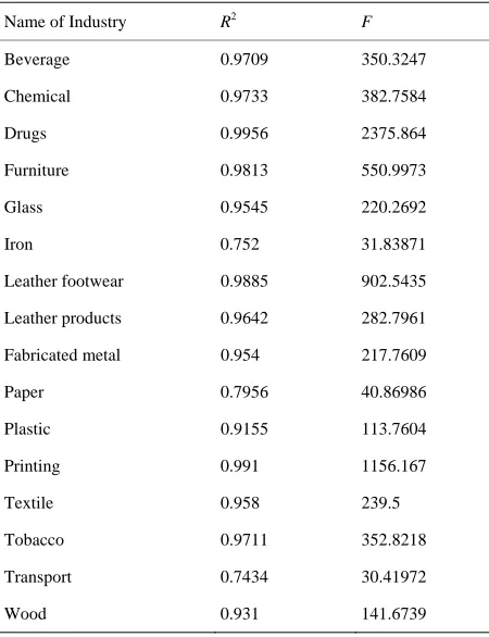
From Table 3, we observe that is highly signifi-

cant for all the manufacturing industries, we can say that the intrinsically nonlinear model (2.2) is fitted well ac-

cording to the null hypothesis 

he e f g t with additive error term (intrinsically nonlinear) of the

indus-der study

[image:7.595.62.539.428.733.2]

.

Table 2. T stimates o Cobb-Dou las produc ion function

tries un .

Industry name Intercept p-value Capital elasticity (2) p-value Labor elasticity (3) p-value Return to scale (23)

2 3

1



 

 

Bever ge 5.a 848951 0.0650 0.683362 0.0001 0.230199 0.0458 0.913561 1.094618

Chemical 6.552999 0.0720 0.567255 0.0001 0.239483 0.0113 0.806738 1.23956

r footwear e

g 47

t

Drugs 1.418816 0.0107 0.578490 0.0350 0.583740 0.0321 1.16223 0.860415

Furniture 0.136145 0.3751 1.583382 0.0001 0.323816 0.0001 1.907198 0.524329

Glass 10.858785 0.0048 0.446118 0.0001 0.267905 0.0792 0.714023 1.400515

Iron 5.432328 0.5702 0.317029 0.0641 0.825566 0.0265 1.142595 0.875201

Leathe 9.975966 0.0001 0.168618 0.1296 0.851867 0.0001 1.020485 0.979926

Leath r products 149.5248 0.0008 0.273520 0.0293 0.396121 0.0185 0.669641 1.493337

Fabricated metal 1.560328 0.1357 0.282128 0.0753 0.979802 0.0001 1.26193 0.792437

Paper 36.90303 0.4661 0.154744 0.5083 0.593256 0.0002 0.748 1.336898

Plastic 10.04537 0.0001 0.081875 0.5527 0.962046 0.0001 1.043921 0.957927

Printin 0.761334 0.0090 1.062223 0.0001 0.215724 0.0007 1.2779 0.782505

Textile 33.44288 0.2979 0.503446 0.0001 0.237309 0.0874 0.740755 1.349974

Tobacco 5.828218 0.1361 0.867991 0.0001 0.257396 0.0001 1.125387 0.888583

Transpor 35.21922 0.4605 0.037898 0.7996 0.873132 0.0124 0.91103 1.097659

Wood 45.73787 0.0789 0.054236 0.6731 0.566334 0.0001 0.62057 1.611422

(8)

[image:8.595.59.284.112.405.2]

Table 3. The values of test statistic of intrinsically nonlinear model for selected manufacturing industries.

ndustry F

Name of I R2

Beverage 0.9709 350.3247

Chemical 0.9733 382.7584

Drugs 0.9956 2375.864

13 .9973

footwear

ted metal

o rt

Furniture 0.98 550

Glass 0.9545 220.2692

Iron 0.752 31.83871

Leather 0.9885 902.5435

Leather products 0.9642 282.7961

Fabrica 0.954 217.7609

Paper 0.7956 40.86986

Plastic 0.9155 113.7604

Printing 0.991 1156.167

Textile 0.958 239.5

Tobacc 0.9711 352.8218

Transpo 0.7434 30.41972

Wood 0.931 141.6739

In order to forecast the production of manufacturing

industries, we use the production function (Table 4).

NCES

[1] C. W. Cobb and P. H. Douglas, “A Theory of Produc-

Econ 1928,

.

[ . Murti and V. K. Sastry, “Production Functions for Indian Industry,” Econometrica, Vol. 25, No. 2,

-221. doi:10.2307/1910250

Table Estimated intrinsic nonlinear uglas

p n functions for t ufacturin ie

de

f industry ed intrinsically nonlinear

C uglas produc n

4. ally Cobb-Do

roductio he man g industr s

un-r study.

Name o Estimat

obb-Do tion functio Beverage P5.848951K0.683362L0.230199

Chemical 0.567255 0.239483

6.552999

P K L

Drugs 0.578490 0.583740

8816

P K L

85

0.317029 0.825566

28

P K L

footwear 0.168618 0.851867

66

P K L

0.27352 0.396121

9.5248

P K L

ted me 0.282128 0.979802

0328

P K L

0.154744 0.593256

03

P K L

0.081875 0.962046

4527

P K L

1.062223 0.215724

34K L

0.503446 0.237309

88

P K L

o 0.867991 0.257396

18

P K L

rt 0.037898 0.873132

22

P K L

Wood 0.054236 0.566334

87

P K L

1.41



Furniture 1.583382 0.323816

0.136145

P K L

0.446118 0.267905

P K L

Glass 10.8587

Iron 5.4323

Leather 9.9759

Leather products 14

Fabrica tal 1.56

Paper 36.903

Plastic 10.0

Printing P0.7613

Textile 33.442

Tobacc 5.8282

Transpo 35.219

45.737



REFERE

tion,” American

pp. 139-165

omic Review, Vol. 18, No. 1, 2] V. N

1957, pp. 205

[ . Wu, “Estimation of the Cobb-Douglas Production

Econometrica, Vol. 43, No. 4, 1975 doi:10.2307/1913082

3] D.-M Function,” 744.

, pp.

739-[4] S. M. Goldfeld and R. E. Quandt, “The Estimation of Cobb-Douglas Type Functions with Multiplicative and Additive,” International Economic Review, Vol. 11, No. 2, 1970, pp. 251-257. doi:10.2307/2525667

[5] S. M. Goldfield Methods of

Econometrics, ion Company, Am-

and R. E. Quandt, “Nonlinear ” North-Holland Publicat sterdam, New York, 1976.

[6] H. H. Kelejian, “The Estimation of Cobb-Douglas Type Functions with Multiplicative and Additive Errors: A Further Analysis,” International Economic Review, Vol. XIII, 1972, pp. 179-182. doi:10.2307/2525915

[7] M. Brown, “On the Theory and Measurement of Techno- logical Change,” Cambridge University Press, Cambridge, 1966.

[8] B. Sandelin, “On the Origin of the Cobb-Douglas Produc- tion Function,” Economy and History, Vol. 19, No. 2, 1976, pp. 117-125.

doi:10.1080/00708852.1976.10418933

[9] P. Samuelson, “Paul Douglas’s Measurement of Produc- tion Functions and Marginal Productivities,” Journal of Political Economy, Vol. 87, No. 5, 1979, pp. 923-939. doi:10.1086/260806

[10] A. A. Cheema, “Productivity Trends in the Manufacturing Industries,” The Pakistan Development Review, Vol. 17, No. 1, 1978, pp. 55-65.

[11] A. R. Kemal, “Substitution Elasticities in the Large Scale Manufacturing Industries in Pakistan,” The Pakistan De- velopment Review, Vol. 20, No. 1, 1991, pp. 11-36. [12] S. Wizarat, “Sources of Growth in Pakistan’s Large Scale

Manufacturing Sector: 1955-56 to 1980-81,” Pakistan Economic and Social Review, Vol. 21, No. 2, 1989, pp. 139-159.

[13] M. Azhar and S. Khan, “Effects of Tax Holidays on In- vestment Decisions,” The Pakistan Development Review, Vol. 13, No. 4, 1974, pp. 245-248.

[14] E. Bond, “Tax Holidays and Industry Behavior,” The Review of Economics and Statistics, Vol. 63, No. 1, 1981, pp. 88-95. doi:10.2307/1924221

[15] G. M. Radhu, “The Relation of Indirect Tax Changes to Price Changes in Pakistan,” The Pakistan Development

Functions for Indian Manufacturing Industries,” Indian Review, Vol. 5, No. 1, 1965, pp. 54-63.

[image:8.595.61.283.452.732.2]

(9)

Journal of Industrial Relations, Vol. 15, No. 3, 1980, pp

conomics,” Oxford University Press, Oxford,

Survey Data,” . 395-409.

[17] I. M. D. Little, D. Mazumdar and J. M. Page Jr.,“Small Manufacturing Enterprises: A Comparative Study of India and Other E

1987.

[18] J. M. Page Jr., “Firm Size and Technical Efficiency: Ap- plication of Production Frontiers to Indian

Journal of Development Economics, Vol. 16, No. 1-2, 1984, pp. 129-152. doi:10.1016/0304-3878(84)90104-4 [19] T. Bhavani, “Technical Efficiency in Indian Modern

d B. Ghosh, “Intertemporal Efficiency Var Small Scale Sector: An Application of Frontier Produc- tion Function,” Indian Economic Review, Vol. 26, No. 2, 1991, pp. 149-166.

[20] B. Goldar, “Unit Size and Economic Efficiency in Small Scale Washing Soap Industry in India,” Artha Vijnana, Vol. 27, No. 1, 1985, pp. 21-40.

[21] C. Neogi an ia-

tions in Indian Manufacturing Industries,” Journal of Pro- ductivity Analysis, Vol. 5, No. 3, 1994, pp. 301-324. doi:10.1007/BF01073913

[22] Y. Nikaido, “Technical Efficiency of Small-Scale

Indus-e

tent of Productivity Growth in Swed-try: Application of Stochastic Production Frontier Model,”

Economic and Political Weekly, Vol. 39, No. 6, 2004, pp. 592-597.

[23] B. Goldar, “Relative Efficiency of Modern Small Scal Industries in India,” In: K. B. Suri, Ed., Small Scale En-terprises in Industrial Development, Sage Publication, New Delhi, 1988.

[24] B. Carlsson, “The Con

ish Manufacturing,” Research Policy, Vol. 10, No. 4, 1981, pp. 336-355. doi:10.1016/0048-7333(81)90018-4 [25] M. Daly, I. Gorman, G. Lenjosek, A. MacNevin and W.

Phiriyapreunt, “The Impact of Regional Investment In- centives on Employment and Productivity: Some Cana- dian Evidence,” Regional Science and Urban Economics, Vol. 23, No. 4, 1993, pp. 559-575.

doi:10.1016/0166-0462(93)90047-I

[26] B. Contini, R. Revelli and S. Cuneo, “Productivity and Imperfect Competition: Econometric Estimation from Panel- Data of Italian Firms,” Journal of Economic Behavior & Organization,Vol. 18, No. 2, 1992, pp. 229-248.

doi:10.1016/0167-2681(92)90029-B

[27] J. K. Mullen and M. Williams, “Explaining Total Factor Productivity Differentials in Urban Manufacturing,” Jour- nal of Urban Economics,Vol. 28, No. 1, 1990, pp. 103- 123. doi:10.1016/0094-1190(90)90045-O

[28] W. L. Weber and B. R. Domazlicky, “Total Factor Pro- ductivity Growth in Manufacturing: A Regional Approach Using Linear Programming,” Regional Science and Ur- ban Economics,Vol. 29, No. 1, 1999, pp. 105-122. doi:10.1016/S0166-0462(98)00013-1

[29] J. Nemoto and M. Goto, “Productivity, Efficiency, Scale Economies and Technical Change:

tion Analysis of TFP Applied to the

A New Decomposi- Japanese Prefec- tures,” Journal of the Japanese and International Econo-

mies, Vol. 19, No. 4, 2005, pp. 617-634. doi:10.1016/j.jjie.2005.10.006

[30] N. Maniadakis and E. Thanassoulis, “A Cost Malmquist Productivity Index,” European Journal of Operational Research,Vol. 154, No. 2, 2004, pp. 396-409.

doi:10.1016/S0377-2217(03)00177-2

[31] A. Radam, “Efficiency and Productivity of the Malaysian Food Manufacturing Industry,1983-2000,”Universiti Pu- tra Malaysia, 2007.

[32] B. Goldar, V. S. Renganathan and R. Banga, “Owne and Efficiency in Engineering Firms: 1

rship 990-1991 to 1999-

084-5

2000,” Economic and Political Weekly, Vol. 39, No. 5, 2004, pp. 441-447.

[33] S. V. Lall and G. C. Rodrigo, “Perspective on the Sources of Heterogeneity in Indian Industry,” World Development, Vol. 29, No. 12, 2001, pp. 2127-2143.

doi:10.1016/S0305-750X(01)00

y of Con-

udy,” Managerial Auditing Journal,

ific Basin Financial Markets and

[34] K. Mukherjee and S. C. Ray, “Technical Efficiency and Its Dynamics in Indian Manufacturing: An Inter-State Analysis,” Working Paper, No. 18, Universit

necticut, Storrs, 2004.

[35] Md. Z. Hossain, M. I. Bhatti and Md. Z. Ali, “An Econometric Analysis of Some Major Manufacturing In-dustries: A Case St

Vol. 19, No. 6, 2004, pp. 790-795.

[36] C.-P. Lin, “The Application of Cobb-Douglas Production Cost Functions to Construction Firms in Japan and Tai- wan,” Review of Pac

Policies (RPBFMP), Vol. 5, No. 1, 2002, pp. 111-128. doi:10.1142/S0219091502000663

[37] M. Jung, K. Lee and K. Fukao, “Total F of Korean Firms and Catching up

actor Productivity with the Japanese

earch on International Economic

ected Manufacturing

li-llege Publishers, New

gladesh Bureau of Statistics, Statistics Divi-

ion, Firms,” Seoul Journal of Economics, Vol. 20, No. 1, 2008, pp. 93-139.

[38] D. A. Hashim, “Cost and Productivity in Indian Textiles- Indian Council for Res

Relations. Multan District,” Journal of Quality and Tech- nology Management, Vol. 5, No. 2, 2009, pp. 91-100. [39] Md. Z. Hossain and K. S. Al-Amri, “Use of Cobb-Doug-

las Production Model on Some Sel

Industries in Oman,” Education, Business and Society:

Contemporary Middle Eastern Issues, Vol. 3, No. 2, 2010, pp. 78-85.

[40] R. Ramanathan, “Introductory Econometrics with App cations,” 3rd Edition, Harcourt Co

York, 1995.

[41] “Statistical Year Book,” 5th Edition, 7th Edition, 16th Edition, 18th Edition, 21st Edition, 22nd Edition, 24th Edition, Ban

sion, Ministry of Planning, Dhaka, 1984, 1986, 1995, 1997, 2000, 2001, 2003.