Power system state estimation and probabilistic loadflow analysis

A thesis

presented for the degree of

Doctor of Philosophy in Electrical Engineering

in the

University of Canterbury,

Christchurch, New Zealand

by

E.P.M. BROWN B.E. (HONS), M.E.

"Never take anything for granted"

Benjamin Disraeli 1804-1881

CONTENTS

List of Illustrations List of Tables

List of Principal Symbols Abstract

Acknowledgements

CHAPTER 1

CHAPTER 2

INTRODUCTION

REVIEW OF TRANSMISSION LINE MODELLING AND

WEIG~TED LEAST SQUARES STATE ESTIMATION CONCEPTS

2.1 2.2 2.3 2.4 2.5 Introduction

Transmission line model and power system measurement equations Measurement noise

Weighted least squares static state estimation Other methods of state estimation

Page xL xvL xxvi. xxvii. xxviii. 1 14 14 17 19 20

2.5.1 Dynamic tracking state estimators 20

CHAPTER 3

2.5.2 Transformation-based state estimators 21

2.5.3 Linear programming-state estimators 22

2.5.4 Sequential state estimators 22

2.6 2.7

Comparison of other methods of state estimation with W.L.S. Conclusion

FAST, OPTIMAL STATE ESTIMATION WITH PSEUDO LINE-FLOW CREATION FROM INJECTION MEASUREMENTS

3.1 3.2

Introduction

Possible creation of pseudo line-flows from injection measurements

3.2.1 Method 1 3.2.2 Method 2

3.3 Modifications to the information matrix

to give sparse structures 3 . 3 . 1 Me thod 3

3.3.2 Method 4

22 23

24 '

CHAPTER 4

3.4

3.5

3.6

3.7

Optimality of the estimates obtained from pseudo line-flow creation or from modifications to the information matrix

Converge~ce properties of W.L.S.

with and w~thout pseudo line-flow creation

or modification to the information matrix 3.5.1 Method 1

3.5.2 Method 2 3.5.3 Method 3 3.5.4 Method 4

Methods of improving the convergence of W.L.S. when pseudo line-flow creation and

information matrix modifications are used Results

3.7.1 Discussion of results and selection

Page 31 31 32 33 33 34 36 36

of the best method for further testing 43

3.7.2 Reasons for the dramatic speed improvement when pseudo line-flow

creation is used 44

3.8 Further refinements to method (1)

which do not degrade optimality

3.9 Two-stage optimal W.L.S. estimation

with pseudo line-flow creation

3.10 Testing the refinements to method (1)

45

48

49 3.10.1 Performance of methods of improving

convergence without degrading optimality 49

3.11

3.10.2 Fast, optimal two-stage W.L.S. state estimation with pseudo line-flow

creation 53

3.10.3 Effect of variance conditioning on estimate accuracy when measurement

noise is present 54

3.10.3.1 Nominal measurement noise ~<3a)

3.10.3.2 Bad data

(>3a.)

Conclusions

54 56

58

REVIEW AND CONVERGENCE ANALYSIS OF DECOUPLED AND FAST DECOUPLED STATE ESTIMATION TECHNIQUES

4.1 4.2 4.3

Introduction

p-e,

Convergence analysis for state estimation

CHAPTER 5

CHAPTER 6

4.4 Summary of possible P-8, Q-v decoupling

and fast decoupling schemes

4.4.1 Algorithm P-8, Q-v decoupling

4.4.1.1 Horisberger et al.

type decoupling 4.4.1.2 'Masiello and Horton

type decoupling 4.4.2 Modal P-8, Q-v decoupling

, Page

67 67 67 79 85

4.4.2.1 Garcia et al. type decoupling 85

4.4.2.2 Couch et al. type decoupling 95

4.5

4.6

4.7

4.4.3 Other fast decoupling schemes Assumptions inherent in the

methods of decoupling presented

Accuracy of the P-8. Q-v decoupling schemes Conclusion

FAST DECOUPLED STATE ESTIMATION WITH PSEUDO LINE-FLOW CREATION FROM INJECTION MEASUREMENT

5.1 5.2

5.3

Introduction

Performance of fast decoupled W.L.S. state estimation with pseudo line-flow creation Conclusion

FAST IDENTIFICATION OF BAD DATA IN POWER SYSTEM TRACKING STATE ESTIMATION

6.1 6.2

6.3

Introduction

Bad data detection and identification 6.2.1 J(x) test

6.2.2 Weighted residual test 6.2.3 Normalised residual test Test results

6.3.1 Verification of mathematical removal technique

6.3.2 Performance of bad data handling techniques

6.3.3 Effect of modifying the variance

100 109 110 112 114 115 117 119 120 120 120 120 124 125 125

when treating bad data 129

6.4

6.3.4 Performance of bad data "replacement" techniques under conditions where

removal cannot be attempted 130

CHAPTER 7

CHAPTER 8

INCLUSION OF H.V.D.C. LINKS INTO A.C. POWER SYSTEM STATE ESTIMATION

7.1 7.2

Introduction

H.v.d.c. link model

7.2.1 Selection of a suitable h.v.d.c.

Page

136 137

link state space 137

7.2.2 H.v.d.c. link measurement equations 140

7.2.3 Effect of approximation error

on the h.v.d.c. link model 144

7.2.4 "Minimal-state" h.v.d.c. link state vector realization

7.2.5 Comparison of minimal approximation error and minimal state h.v.d.c. link state vector realizations

7.3 Performance of the combined multi

7.4

7.5

a.c. -h.v.d.c. state estimator

7.3.1 Effect of retaining a.c. system slack (reference) buses

7.3.2 Minimum h.v.d.c. link observability condition

7.3.3 Additional pseudomeasurements 7.3.4 Geographic partitioning of

the h.v.d.c. link 7.3.5 Performance results

Fast decoupled multi a.c. -h.v.d.c. state estimation

7.4.1 Method 1 7.4.2 Method 2 7.4.3 Method 3 Conclusion

ACCURATE REPRESENTATION OF COMMUTATION OVERLAP A. C. - H V D. C. STATE ESTIMATION AND LOADFLOWS

8.1

8.2

8.3

Introduction

Assu~ptions made in the derivation of

the approximate h.v.d.c. link model Error effects in the approximate model h.v.d.c. link representation

8.4 Inclusion of exact h.v.d.c. link models

in a.c. power system state estimation

CHAPTER 9

8.5

8.6

8.7

8.4.1 Performance results 8.4.2 Minimum h.v.d.c. link

observability conditions 8.4.2.1 Performance results

Exact h.v.d.c. link estimates from approximate h.v.d.c. link model state estimation

8.5.1 Performance results

8.5.1.1 Redundant measurement conditions

8.5.1.2 Minimum h.v.d.c. link measurement observability

conditions

8 • 5 . 1. 3 Mul t i a. c. - h • v . d • c . loadflow conditions Validity of convertor relationships under fault conditions when u > 600 Conclusion Page 172 172 175 177 180 180 180 180 183 184

USE OF AVAILABILITY DATA IN STATE ESTIMATION OPERATION AND OPTIMAL METER PLACEMENT DESIGN

9.1 9.2 9.3

9.4

Review of minimum observability criteria for power system state estimation

Availability analysis

9.3.1 Inclusion of zero injection pseudomeasurements

9.3.2 "Local redundancy" versus "No. of link measurements"

Detailed nodal estimate availability analysis Review of optimal meter placement methods Optimal meter placement

185 187 188 197 201 203 207 210

9.6.1 Optimization constraints 210

9.6.2 Statement of the maximization problem 213

9.6.3 Steps in the optimum meter

placement design 213

Comparison betw'een the "power of the J (x) " test and availability-based meter placement design

Conclusion

CHAPTER 10 HIERARCHICAL STATE ESTIMATION OF A COMBINED ELECTRICAL-HYDROTURBINE AND OPEN CHANNEL

HYDRO CANAL SYSTEM - FEASIBILITY INVESTIGATIONS

10.1 Introduction

10.2 Structure of the combined electrical/ hydraulic state estimator

10.3 Electrical power system tracking state estimation

10.4 Model for the hydroturbine portion of a hydro generating unit

10.4.1 10.4.2

Local hydro turbine dynamic estimation

Local resid~al analysis

10.5 Model of the electrical part of a hydro generating unit

10.6

10.5.1 Rotor angle estimation

Test simulation results 10.6.1

10.6.2

Example 1

Example 2 - Rotor angle estimation 10.7 Model for an open channel hydrocanal

10.7.1 10.7.2

10.7.3

10.7.4

Open channel transient flow Implicit method for solving open channel flow dynamics A dynamic model suitable for a Kalman filter

Structure of the linearized hydrocanal Kalman filter 10.8 Performance results

10.8.1

10.8.2

Accuracy of the dynamic hydro canal model

Dependence of the Kalman filter gain on the flow conditions 10.8.2.1 Variation of K with

measurement set composition

Page 218 222 225 226 230 231 232 233 234 237 239 242 245 246 247 250 251 251 253

for problem 1 (1jJ::::: 0.6) 253

10.8.2.2 Variation of K with

measurement set composition

for problem 2 (1jJ::::: 0.6) 254

10.8.2.3 Varying flow condition (1jJ=0.6)

10.8.2.4 Effect of varying 1jJ 10.8.2.5 Large scale system

Kalman gain calculation

257 257

CHAPTER 11

CHAPTER 12

10.8.3 Kalmap filter tracking results

10.8.3.1 Simulation 1

10.8.3.2 Simulation 2

10.8.3.3 Simulation 3

10.8.3.4 Simulation 4

10.8.3.5 Simulation 5

10.8.3.6 Simulation 6

10.8.3.7 Simulation 7

10.8.3.8 Simulation 8

10.8.3.9 Simulation 9

10.8.3.10 Simulation 10 10.8.3.11 Simulation 11 10.8.3.12 Simulation 12 10.8.3.13 Simulation 13 10.8.3.14 Simulation 14

10.9 Conclusion

STATISTICAL TECHNIQUES IN LOADFLOW STUDIES

11.1 11.2 11.3

Introduction

Review of stochastic loadflow concepts Conclusion

REPRESENTATION OF NON-GAUSSIAN PROBABILITY DISTRIBUTIONS IN STOCHASTIC LOADFLOW STUDIES BY GAUSSIAN SUM APPROXIMATIONS

12.1 12.2 12.3 12.4 12.5 12.6 Introduction

Gaussian sum approximation Test system analysis

12.3.1 Comparison between probabilistic and stochastic loadflow results 12.3.2

12.3.3

P-

e,

Effect of nodally dependent real and reactive injection non-gaussian p.d.L's

Lower order gaussian sum approximations Selection of non-gaussian long term generation data

CHAPTER 13 INCLUSION OF H.V.D.C. LINKS IN A.C. STOCHASTIC LOADFLOW STUDIES

CHAPTER 14

REFERENCES APPENDICES Al A2 A3 A4 AS 13.1 B.2 Introduction

Specification of a multi

a.c. -h.v.d.c. stochastic loadflow

13.3 Uses for the multi

a. c. - h. v. d. c. stochastic loadflow

13.4 Multi a.c. -h.v.d.c. stochastic

loadflow test results 13.4.1 Uncorrelated multi

a. c. - h. v. d. c. loadflow data 13.4.2 Correlated multi

a.c. -h.v.d.c. loadflow data

13.5 Conclusion

CONCLUSIONS

Optimality of estimates obtained from pseudo line-flow creation

Properties of estimates resulting from pseudo line-flow creation using method (2)

A2.1 Estimation error

Ox

A2.2 Variance of A x

Convergence analysis of W.L.S. with and without pseudo line-flow creation or information matrix modification

A4.1 W.L.S. state estimation

A4.2 Method (1)

A4.3 Method (2)

A4.4 Method (3)

A4.5 Method (4)

Invariance of Couch et ai.'s simultaneous update

(1.4.1) decoupling with respect to variations in the ratio of R-1 to R-1

-p -q

APPENDICES

A6

A7

A8

Effect of multiple bad data on the EN and Ew tests

A6.1 Single bad data

A6.2 Multiple non~interacting bad data

A6.3 Multiple interacting bad data

A6.4 Example involving the EN and Ew tests

Mathematical "removal" of measurement data

Derivation of measurement equations for Em' P2- 3, Q2-3 and 111_{2_3}

A9 Derivation of h.v.d.c. link "minimal-state" realization measurement equations

AIO

All Al2

Al3

Al4

To show the exact relationship between a, Wand 0 is monotonically increasing for a < x < 1T -a

Approximate nodal estimate unavailability, A. J. Rotor angle estimation

Derivation of unsteady open channel flow momentum and continuity equations

Implicit trapezoidal numerical integration

Page

368 368 369

370 370

373

375

377

379

382

388

FIGURE 1.1 1.2 1.3 1.4 2.1 3.1 3.2 3.3 3.4 3.5 3.6 3.7 4.1 4.2 4.3

4.4

LIST OF ILLUSTRATIONS

Typical control center operation. (Schweppe and Handschin, 1974)

The static state estimator as a buffer. (Schweppe and Handschin, 1974)

Time interval in which monitoring and control functions must be performed.

(Handschin and Bongers, 1975)

Basic operation of the state estimator.

(Schweppe and Handschin, 1974)

TI-equivalent circuit for a transmission line. (Turner, 1980)

Structure of the "difference" matrix for method (3)

Structure of the "difference" matrix for method (4)

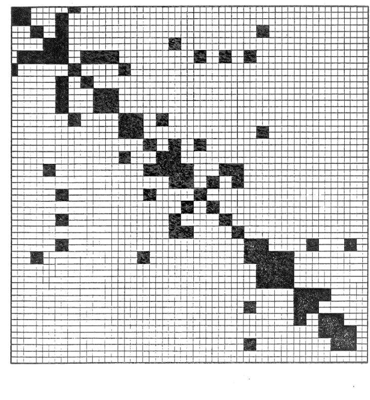
5 bus test system (Stagg and El-Abiad, 1968)

Information matrix when 29 (Pi +Qi) injection measurements are present Information matrix when 74 (Pi + Qi) line-flow measurements are present

Optimal estimation using 2 stage W.L.S. with pseudo line-flow creation

Convergence characteristics when RaL =(1.25 azt' )2jqi and Ra :::: a ,2

R '

Horisberger-type ·decoupling: unified (1.1.1)

Horisberger-type decoupling: unified

with constant gain (1.1.3)

Horisberger-type decoupling: sequential (1.1.2)

Horisberger-type decoupling: sequent~al

with constant gain (1.1.4)

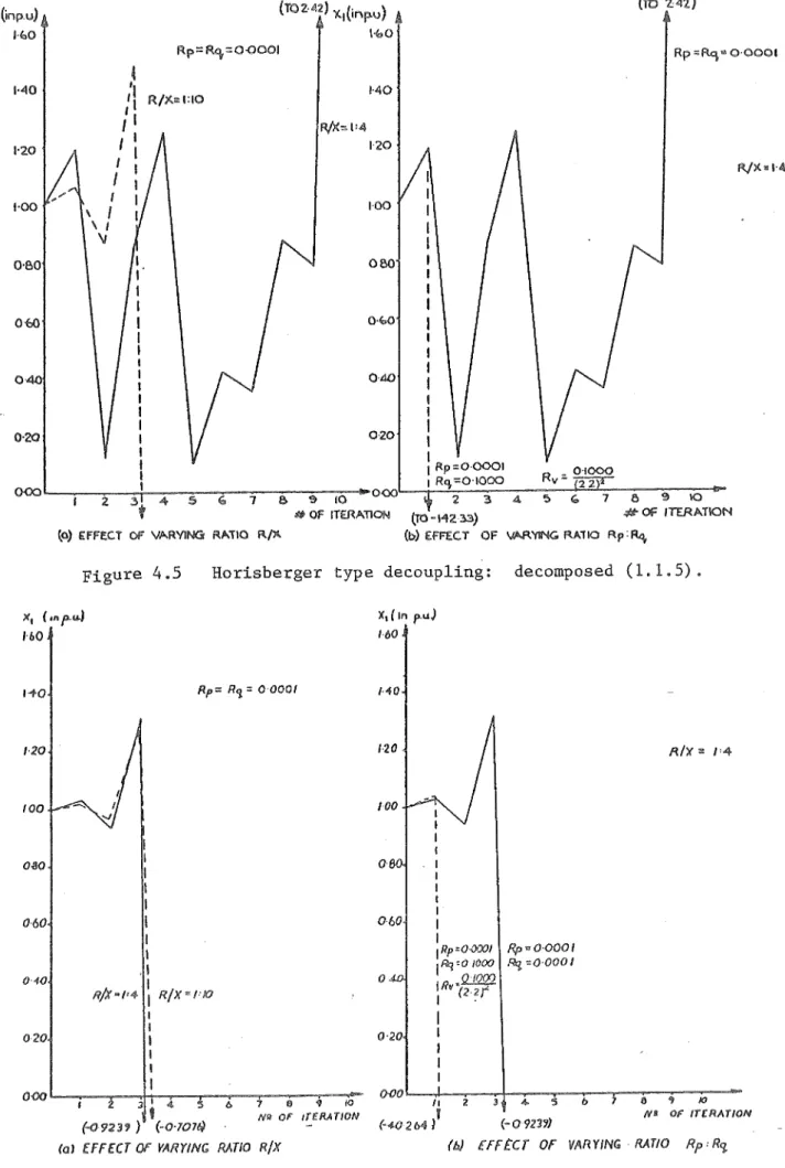
Horisberger-type decoupling: decomposed (1.1.5)

Horisberger-type decoupling: decomposed

with constant gain (1.1.6)

FIGURE

Masiello-type decoupling: unified (1.2.1)

Masiello-type decoupling: unified with

constant gain (1.2.3)

Masiello-type decoupling: sequential (1.2.2)

Masiello-type decoupling: sequential with

constant gain (1.2.4)

Masiello-type decoupling: decomposed (1.2.5)

Masiello-type decoupling: decomposed with

constant gain (1.2.6)

Garcia et al. type decoupling: unified (1.3.1)

Garcia et al. type decoupling: unified with

constant gain (1.3.3)

Garcia et ale type decoupling: sequential (1.3.2)

Garcia et al. type decoupling: sequential with

constant gain (1.3.4)

Garcia et al. type decoupling: decomposed (1.3.5)

Garcia et al. type decoupling: decomposed with

constant gain (1.3.6)

Couch et ale type decoupling: unified (1.4.1)

Couch et al. type decoupling: unified with

constant gain (1.4.3)

Couch et al. type decoupling: sequential (1.4.2)

Couch et al. type decoupling: sequential with

constant gain (1.4.4)

Couch et ale type decoupling: decomposed (1.4.5)

Couch et ale type decoupling: decomposed with

constant gain (1.4.6)

Bermundez and Brameller fast decoupling (1.5.1)

Bermundez and Brameller fast decoupling -decomposed (1.5.2)

6.1 Effect of variance conditioned bad data

"replacement" techniques

FIGURE

7.1 H.v.d.c. link and equivalent circuit

7.2 H.v.d,c. link Jacobian structure for minimal

error realization (78 non-zero elements)

7.3 7.4 7.5 7.6 8.1 8.2

H.v.d.c. link Jacobian structure for minimal state realization (122 non-zero elements)

Multi a.c. -h.v.d.c. test system

Partitioned h.v.d.c. link equivalent circuit

3 a.c. - 2 h.v.d.c. link test system

Error in value of ~m at normal rectifier operationg conditions

Rectifier commutation when (a) a small and (b) a large

8.3 Flow diagram for approximate h.v.d.c. link model

a.c. -h.v.d.c. state estimation algorithm with exact residuals

9.1 9.2 9.3 9.4 9.5 9.6 9.7 10.1 10.2 10.3 10.4 10.5

Observability of 5 bus test system with an, observable measurement set

Observability of 5 bus test system with an unobservable measurement set

I.E.E.E. test network with optimal meter configuration (Hands chin and Bongers, 1975)

Node 12 and its nearest neighbours

Node 4 and its nearest neighbours

I.E.E.E. test network with first meter configuration (Hands chin and Bongers, 1975)

Transition diagram for node 1

"Possible" 220 kV measurements on Upper Waitaki system

"Possible" 33 kV electrical measurements

Location of Tekapo canal height and flow measurements

Two level "static-dynamic" state estimator of network hydrocanal and power plant states when s hydrocanals and m hydrogenerators are present

Hierarchical estimation scheme with centralized tracking estimator and local dynamic estimators for thermal

power plants (1), large loads (2), tie lines (3), hydro-power (4) and hydrocanal states (5)

FIGURE 10.6 10.7 10.8 10.9 10.10 10.11 10.12 10.13 10.14 10.15 10.16 10.17 12.1 12.2 12.3 12.4 12.5 12.6 12.7 12.8 12.9 12.10 12.11 12.12

Functional diagram of the Kettle power station turbine and governor equipment

Transient model of the electrical part of a generating unit

Test network with two hydrogenerators, three loads and one open channel hydrocanai

Frequency deviation after 0.2 p.u. incremental increase in load (no measurement noise and Tp = 0.2)

Frequency deviation after 0.2 p.u. incremental noise in load (measurement noise and T~ =0.2)

Frequency deviation after 0.2 p.u. incremental increase in load (measurement noise and T?

=

Rotor angle estimation; measurement noise and TF = 0.02

Rapidly varied unsteady flow (Chow, 1959)

Discretization of the open channel (Wylie and Streeter, 1978)

Discretization of the open channel for Kalman filter implementation

Initial flow conditions for problem 1

Initial and final flow conditions for problem 2

Gaussian sum reconstruction for

V

Gaussian sum reconstruction for _PS-6

Gaussian sum reconstruction for _Q7-9

Gaussian sum reconstruction for Q₃

Gaussian sum reconstruction for Q'

3 (= Q3 +Q17)

Gaussian p.d.L "stochastic loadflow" for P4-7 Gaussian p.d .f. I1s tochastic loadflow" for

P 3-4

Decoupled gaussian sum reconstruction for _{P5- 6}

Decoupled gaussian sum reconstruction for _P

4- 7 Decoupled gaussian sum reconstruction for Q7-9 Decoupled gaussian sum reconstruction for '14

Detailed decoupled gaussian sum reconstruction for Q7-9

FIGURE 12,13 12,14 12.15 12.16 12,17 12.18 12.19 12.20 12.21 12.22 12.23 13.1 Al0.l All.1 All.2 A13.1 A14.1 A14.2

Nodal-dependent gaussian sum reconstruction for V 4 Nodal-dependent gaussian sum reconstruction for P

S-6

Nodal-dependent gaussian sum reconstruction for Q7-9

Nodal-dependent gaussian sum reconstruction for Q

3 Lower order gaussian sum reconstruction for P

3-4 Lower order gaussian sum reconstruction for P

4-7

Lower order gaussian sum reconstruction for PS-6

Lower order gaussian sum reconstruction for Q7-9

Lower order gaussian sum reconstruction for V₄

Lower order gaussian sum reconstruction for

Q

Continuous "equivalent" binomial distribution for the discrete binomial distribution at node 1

Multi a.c. -h.v.d.c. stochastic loadflow test system

"Monotonic" increasing profile of f(x)

Sample a.c. system

Node 12 and its nearest neighbours isolated from the a.c. system

Control volume for application of the unsteady

momentum equation (Wylie and Streeter, 1978)

Single step trapezoidal integration

Multi step trapezoidal integration

TABLE

3.1

3.2

3.3

3.4

LIST OF TABLES

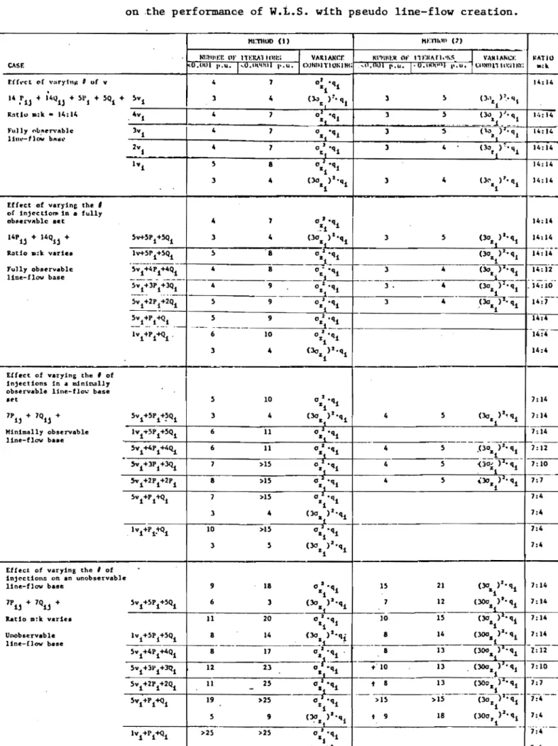
Effect of different measurement configurations (p:k ratio) on the p.erformance of W.L.S.

with pseudo line-flow creation

Effect of different measurement configurations (p:k ratio) on the performance of W.L.S.

with information matrix modification

Large scale system performance of W.L.S. with and without pseudo line-flow creation

and information matrix modification

Effect of altering RaL and ~aR by different amounts, when variance conditioned pseudo line-flows (p :k) = 14: 14 present

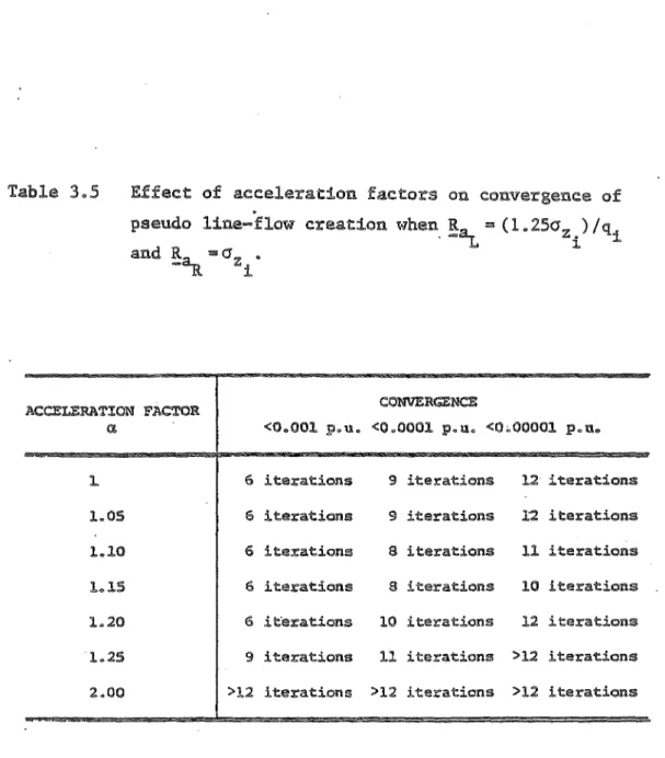
3.5 Effect of acceleration factors on

convergence of pseudo line-flow creation when "RL _::a = (1. 25a z . ) 2 / q . and RaR = a z .

1. l - 1.

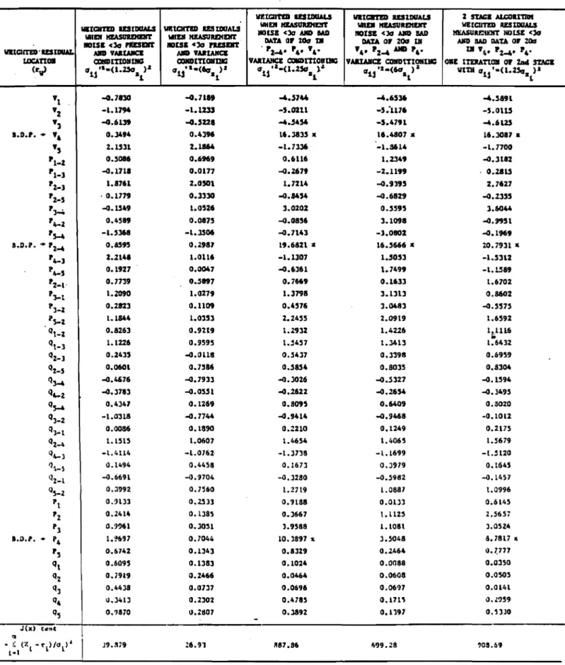
3.6 Estimated degtadation due to variance conditioning

in the presence of noisy measurements (>3a) (in p.u.)

3.7 Detection and identification of bad data when

variance-conditioned pseudo line-flow creation is used

4.1

4.2

4.3

4.4

4.5

4.6

4.7

4.8

Non-zero Jacobian partial derivatives

Different Horisberger et ale type P-8, Q-v decoupling possibilities and their convergence

Different Masiello and Horton type P-8, Q-v decoupling possibilities and their convergence

Different Garcia et ale type P-8, Q-v

decoupling possibilities and their convergence

Different Couch et ale type p-8, Q-v

decoupling possibilities and their convergence

Non-zero Jacobian partial derivatives for Bermundez and Brameller's fast decoupling

Different Bermundez and Brameller type P-8, Q-v decoupling possibilities and their convergence

Accuracy of stable sub-optimal estimation schemes

Comparison of W.L.S. and A.E.P. "line-only" method when pseudo line-flow creation is used

TABLE

5.2

5.3

6.1

Performance of fast decoupled W,L.S. with psuedo line-flow creation (measurement noise free)

30 bus test system performance of fast decoupled W.L.S. with pseudo line-flow creation

Comparison between estimates after mathematical and physical bad data removal

6,2 Change in power system states between

successive measurement scans

6.3

6.4

6.5

6.6

7.1

Comparison of bad data handling methods for different measurement configurations and power system dynamics

Comparison of variance conditioned bad data handling "replacement" methods when measurement system 1 is used

Comparison of bad data handling "replacement" methods when measurement system 1 would be unobservable if

"removal" of bad data was attempted

Comparison of bad data handling "replacement" methods when measurement system 2 would be unobservable if

"removal" of bad data was attempted

Pseudomeasurement non-zero Jacobian terms for the rectifier side

7.2 Jacobian elements for the h.v.d.c. link

measurement equations

7.3 7.4

7.5

Measurement equations for "minimal state" h.v.d.c. link realization

A.c. and h.v.d.c. link parameters

A.c. -h.v.d.c. -a.c. measurement data

Effect of bad data in a.c. terminal measurement, PIS' on the quality of the approximate model h.v.d.c. link estimates of minimal observability conditions

Comparison of h.v.d.c. link estimates with and without geographic partitioning

Measurement breakdown for the a.c. -h.v.d.c. system

A.c. -h.v.d.c. flat start conditions

Comparison of various fast decoupled a.c. -h.v.d.c. stable estimation schemes

TABLE

8.1 Non-zero Jacobian elements for exact h.v.d.c.

link model convertor pseudomeasurement relationships

8.2 Comparison of exact model h.v.d.c. link and approximate

model h.v.d.c. link estimates with and without exact

Page

173

residuals, with moderate measurement redundancy present 174

8.3 Comparison of exact h.v.d.c. link and approximate model

h.v.d.c. link estimates with and without exact residuals of minimum observability conditions

8.4

9.1

Comparison of exact model h.v.d.c. link Newton Ralphson representation in approximate h.v.d.c. link state

estimation algorithms and approximate h.v.d.c. link state estimation for a loadflow measurement set

Nodal availabilities for optimal meter configuration, 14 bus I.E.E.E. test system and effect of communication link failure (one link per node)

9.2 Effect of communication link failure when measurements

from 2 nodes are transmitted through the same link. Optimal meter configuration.

9.3 Nodal availabilities for "first meter" configuration, 14 bus I.E.E.E. test system and effect of communication link failure (one link per node)

9.4 Effect of communication link failure when measurements

from 2 nodes are transmitted through the same link. First meter configuration.

9.5 9.6 10.1 10 .2 10.3 10.4 10.5

Nodal availabilities for optimal meter configuration, 14 bus I.E.E.E. test system and effect of communication link failure (one link per node) when zero injection pseudomeasurement at node 7 is included

Probability of generating observable estimates for the 14 bus optimal meter configuration

Initial conditions for power systems simulation

Power station parameters

Accuracy of the method of characteristics and the implicit Newton method

Comparison of the accuracy of the method of

characteristics and the accuracy of the trapezoidal integration method

Kalman filter gain for the initial flow conditions of problem 1

(til

TABLE 10.6 10.7 10~8 10.9 10.10 10.11 10.12 10.13 10.14 12.1 12.2 12.3 12.4

Kalman filter gain for the initial flow conditions of problem 2 (1jJ::: 0.6)

Kalman filter gain and co-variance matrix for the flow conditions described by problem 3 (1jJ:::::: 0.6)

Kalman filter gain for the flow conditions described by problems 1, 2 and 3 when 1jJ

=

"Approximate" large scale Kalman filter gains for problems 1 and 2

Open channel flow estimates, using problem 1, when the Kalman gain is modified

Open channel flow estimates, using problem 2, when the Kalman gain or the number of

measurements present are modified

Open channel flow estimates, using problem 2, when the integration step length is modified

Open channel flow estimates for problem 1 when a 20 "cell" resolution is used

Open channel flow estimates for problem 2 when a 20 "cell" resolution is used

Convolution components and their weightings

Deterministic data for the expanded I.E.E.E. 14 bus test system

Probabilistic data for the expanded I.E.E.E. 14 bus test system

Individual components of the binomial probability distribution

12.5 Probabilistic data for the S.L.F.:

12.6

12.7

12.8

12.9

Expected values and variances

Gaussian sum approximation component values and their weightings

Comparison of upper and lower limits of S.L.F. and P.L.F. results

Dependent combinations of P

9 and

Q

Normalised non-central moments for non-gaussian distribution for PI' P₂, P₉,

Q

TABLE

12.10

13.1

Minimum values of aI' ~1' aI' ~2' _a2

H.v.d.c. link loadflow specifications

13.2 Possible combinations of h.v.d.c.

link control specifications

13.3

13.4

13.5

13.6 13.7 13.8 A6.1

A6.2

All.1

Expected values of a.c. and h.v.d.c.

long-term oper~ting data

S.L.F. results (uncorrelated data and different h.v.d.c. link control specifications)

S.L.F. test results (uncorrelated data and different initial loadflow data uncertainties)

A.c. correlation weightings

CR .. )

-~J

H.v.d.c. link data correlation weightings

CR .. )

-lJ

Multi a.c. -h.v.d.c. S.L.F. results (correlated data)

Comparison of

EN

Selected segment of the residual sensitivity matrix with and without single and multiple bad data present

Effect of measurement unavailability on the observability of node 12

Page

309

320

321

323

327

329

331

332

333

372

372

LIST OF PRINCIPAL SYMBOLS

The majority of symbols are defined in the text. but for

convenience the principal symbols are redefined below. Some symbols

have more than one meaning. However, the context in which the symbol

is used should clarify any ambiguities.

a

a.c.

A

C.

1

C m

cov(A,B)

d.c.

D

D.L.F.

E

E r

E'

f

f

o

f ref g

transformer ratio

alternating current

cross-sectional area of flow (m2/sec)

availability of device i

unavailability of device i (= 1 - A ) I

susceptance

cost of data acquisition system measurement i

flow constant (= 1.0)

co-variance between dependent events A and B

direct current

"self regulation effect" gain

deterministic loadflow

frequency residual (p.u.)

expectation operator

error in gaussian sum-moment approximation

transient voltage of the hydrogenerator (p.u.)

convertor alternating voltage (pou.)

frequency deviation of the generating unit (p.u.)

nominal frequency (50 Hz)

frequency deviation of the reference generator (p.u.)

gravitational constant (= 9.806)

G

G(x)

h

h.v.d.c.

H

I

I

J

K

m

m. 1.

n

N(O,R)

conductance

R.H.S. matrix of the general state estimator

non-linear measurement function vector {h : h : hd } (mxl)

p q c

high voltage direct current

Jacobian matrix (mxn)

inertia constant of the rotor

current (p.ll.)

identity matrix

information matrix

denotes an imaginary number j

=

residual

Kalman gain matrix

derivative control constant

integral control constant

proportional control constant

3 i2/rr

3/rr

L.R.S. (information) matrix of the general state estimator

- level of variance conditioning

number of measurements

number of nodally dependent gaussian components at node i

non-gaussian moment of order j

gaussian sum approximation moment of order j

number of busbars in the power system

Manning roughness factor

normal distribution with zero mean and variance R

normal distribution with variance

a

probability of event i occurring

p.d.L

P

P.L.F.

P (t)

e

q

Q

r

r.

1

r

m

r w

R

s

s

o

S

S.L.F.

t,T

T

P

T v

probability density function

active power (p.u.)

wetted perimeter of a trapezoidal canal

probabilistic loadflow

incremental electric power demand with time

lateral inflow per unit length of channel

level of variance conditioning

number of lines attached to bus i

probability of event i not occurring (= 1 - p.)

1

number of reactive power or voltage gaussian sum components

flow of water in a canal (m3/sec)

reactive power (p.u.)

measurement residual (~ - ~(~»)

number of active p~wer gaussian sum components

normalised residual

weighted residual

resistance

measurement noise co-variance matrix (m x m)

hydraulic radius (m)

d.c. line resistance

random number (normalised gaussian)

friction term per unit length

channel slope per unit length

complex power P

+

stochastic loadflow

transformer ratio (% off nominal)

time (seconds)

time constant of the pit~t servo

u

v

VL8

w

x,x

x

Xl d

Xfm,Xfn

X , X

m n

y

Y

Z

Z I

a.

1.

p

D,

8

time constant of the hydraulic turbine

commutation overlap angle (= 8 - a)

instantaneous veloc~ty of the fluid (m/sec)

nodal voltage (phase angle referred to slack node)

nodal voltage (phase angle referred to convertor current)

observation error

frequency deviation

residual sensitivity matrix

state vector = {~, v, ~. ~dc} (nxl)

random variable

reactance

transient reactance of the generator unit

filter reactance of rectifier and inverter

commutation reactances at rectifier and inverter

height of water in hydrocanal (m)

admittance (Y =

1.

+

Z

measurement vector {z , z , zdc} (mxl) -q -p

impedance (z - R

+

measurement transformation (pseudo line-flow)

rate of change between successive measurement scans

channel slope

convertor control angle

weighting factor for gaussian sum component

set of all transmission lines connected to bus i

weighting factor

mass density

measurement noise vector (mxl)

o(t)

o.

1.

o

A.

2: -r

2:

-x

j.l

0.

1. w(t)

T

o

e

internal rotor angle w. r. t the frequency generator

probability of no failure or repair,

between measurement scans, of plant i

estimation error

eigenvalue

mean time to failure (MTBF)

network structure vector

residual co-variance matrix

estimation co-variance matrix

mean value

mean time to repair device i

standard deviation of the i th measurement error

model inaccuracies and system noise

unit weight of fluid

shear stress

voltage phase angle referred to slack node

voltage phase angle referred to convertor current

phase angle of convertor alternating voltage

Subscripts and superscripts

dc h.v.d.c. link pseudomeasurement

I imaginary part of a complex variable

k iteration number

m rectifier side of the h.v.d.c. link

-number of measurements

n inverter side of the h.v.d.c. link

number of states in the state vector

p active power measurement partition

q'

r

s

sec

-1

x

T

x

"

x

reactive power measurement partition

real part of a complex variable

h.v.d.c. link pseudomeasurement

secondary side of transformer

inverse of a matrix x

transpose of matrix x

time derivative of x

value of x at time t

general element of matrix x

This thesis investigates the treatment of aposteriori and

apriori uncertainties in power system planning and operation.

Aposteriori uncertainty is treated by power system state

estimators. A survey of existing techniques and their limitations is

described. A method is presented that improves the speed of weighted

least squares state estimation by modifying the structure of injection

measurements to give a very sparse information matrix, the matrix to be

inverted. Used with fast decoupling, this approach yields a very fast

on-line state estimator, capable of handling all types of measurements.

Bad data detection and identification techniques are reviewed

and an improvement based on "mathematical" bad data removal is presented.

The inclusion of h.v.d.c. links into a.c. state estimation is

considered. Decoupling and geographic partitioning of the multi

a.c. -h.v.d.c. state estimator are shown to cause little degradation

in the estimates, and a method of accurately representing commutation

overlap angle is outlined.

Availability analysis in state estimator operation and design

is considered, and applied to optimal meter placement design.

The feasibility of hierarchical central-electrical, local-dynamic

hydroturbine and canal state estimation, based on a linearized Kalman

filter, is investigated.

Apriori uncertainty in long-term future planning studies involving

expected nodal generation and loads can be included in stochastic

load-flows. A method is presented which enables the stochastic loadflow,

which handles only gaussian statistics, to handle non-gaussian

probability distributions via gaussian sum approximations. R.v.d.c.

links are also included in a.c. stochastic loadflows, using both

ACKNOWLEDGEMENTS

I especially wish to thank my supervisor, Dr H.R. Sirisena,

for his enthusiasm a?d guidance throughout this research,

Acknowledgements are also due to Professor J. Arrillaga,

Professor l.R. Wood and Dr A.J. Sutherland for answering my queries,

and to my postgraduate colleages; in particular Messrs B.J. Harker,

M.D. Heffernan and K.S. Turner, for many valuable discussions.

I wish also to thank New Zealand Electricity and the State

Services Commission for their financial assistance and granting of

leave for this study. I also wish to thank Mr C.V. Currie,

Mr W. Wilson, Mr B. Thompson, and the staff of the Christchurch

District Draughting Section of New Zealand Electricity for draughting

all the many figures in this text.

The staff of the Comp.uter Centre of the University of Canterbury

are also to be thanked for their invaluable help, and Mrs A.J. Dellow

for typing this thesis.

Last, but not least, I am indebted to my wife, Lesley, for

her continued patience and encouragement throughout this research

CHAPTER 1

INTRODUCTION

The proliferation of computerised power system control centres which monitor large sets of measurements by remote data acquisition from around the power system is in response to the need for fast, accurate control and restorative procedures. Control centre design is becoming extremely complicated; on-line programs are now available which give updated security analysis, economic dispatch and fault analysis. These programs guide the operator in the choice of

restorative action, maximize the security and economy of generation, and minimize damage and down time caused by a fault. All programs rely on having a clean data base available within the computer from which they can derive decisions. The data base within the computer is regularly updated by new measurement "snapshot" scans of the power system every few minutes. This measurement data updating procedure is intended to continue, on-line, indefinitely without failure. Each snapshot scan may contain 1000 or more individual measurements, and it is likely that, at some time, the raw measurement data arriving at the system control centre may contain bad data; metering errors that result from excessive drift or failure, or failure of communication equipment within the data acquisition system. The presence of such errors in the data base may produce the ~qrong control or alarm action (Schweppe at a.~ •• 1970; Schweppe and Handschin, 1974; Handschin and Bongers, 1975).

measurement errors (see Figure 1.1).

r.trm.-Un1t- comm:l. tmBnt :4a~

Storage optimization Interlace

Maintenance sclwd~n.g

t

Secmri t7 l!IC)n:i. taring and control. _Data

Vol.tage-reactive ~wer control.

:aulD

S!l!AUC S!l!A~E ESTIMA~O:a _I

1

:

Data acquisit~on Da1:a acquisition

Protection ~tect:!.c::m

·r.o~~' control. and _ _ e • • Local. control and

mtch1ng m'fi t clJ,in.g

t

t

I

J

Figure 1.1 Typical control centre operation. Schweppe and Handschin, 1974.)

LoBd predic1::l.cll:: for short

:md. long tlllrm

:3tatis1:ic~

B:!.ll:lJ:lg Operat:lJ:lg Re'Ports

li!:ea.sureoEln1:s .! (meter)

Struct"..uT.l information !.

(break~r ?osit1on etc.)

Parameter valUElS ~

(design data)

1) system state

----eo (nodE! vo~tages)

2) mode~ (structure

and parameter values},

during static conditions'

Figure 1.2 The static state estimator as a buffer. (Schweppe and Handschin, 1974.)

III 0 _E N

IJ! R A. J.

R

E G

I I I 0 N A L

0

I C A

r."

ELD: Economic Loud Diapntch 8M :; Security }'lorli taring SO & Security Optimization VVC: Vo1tagelVar Control

-1h _{'" 3.6} lO~f!ee Iday .. 8.6 lOSfl6c

1111eek _'" 6.1 10₇0eo Imonth :; 1.6 10Ss6e lyear .. 2.2 10 sac

- - - -

-Figure 1.3 Time interval in whicb monitoring and control functions must be performed. (Handschin and Bongers~ 1975.)

,-

-

...

Z Parameter information ~

J

PREl"ILTERING

Plausibility check

Lim 1;' values

-Tills

Ehd

Figure 1.4

etc.

Em'OTHESIZE MODE.1'&

MI!mmIll 1) no stru~l fIIrrors e:=O

--2) no bad data: ~=2 .

3) no parameter errors :!p=Q

Usa !!!,and],to obtain 1l(~) and

valUClU1 for R.

1

ii!S'l!I~TION

Pi:l:ld .!. the 7al.ue of 3 which nw.kel!l

the residual ~-g(!) sma.ll.

D 'r

Cb.eck assumptions tlla1;' :Q, B.=Q. by

asid.ng:: Is r I!IcalL enough?

no

IDENTn'ICATIOrT

Logic to detercine location of' bad

~ta ~ and/or structural errors e

Modify inputs

Basic operation of the state estimator. (Schweppe and Handschin, 1974.)

~

Processing a redundant set of measurement data allows bad data detection and identification schemes to be included in the state estimator

algorithm, to locate and remove any faulty measurement data or circuit disconnect status information (see Figure 1.4) . (Schweppe and Handschin,

The concept of state estimation was first used by Gauss (1777-1855) to process data on the orbits of planetary bodies. Since the late 1950s~ with the beginning of aerospace exploration, state estimators have became more sophisticated in order to dynamically ·monitor noisy measurement data from outer space. The "small-scale"

nature of the aerospace problem has allowed complex state estimation techniques to be used. The power system's application, on the other hand, produces an extremely large scale problem. Some power systems may contain 500 busbars or more. Fortunately, however, power systems usually are weakly intercoupled and as a result most matrix manipulation in power system problems involves sparse matrices. Sparsity techniques can be used to handle these matrices, storing only their non-zero values and location addresses. Sparsity techniques, and the quantum leap in computing speed and power of commercial computers over the last decade, have made power system state estimation a reality (Sugarmann, 1980). However only the simple, static state estimation algorithms which process the current measurement snapshot, taking no account of any dynamics, have achieved any success in the power system's applications. The problem of regularly producing reliable power system state estimates

from noisy on-line data acquisition system measurements is not trivial (Brown and Sirisena, 1981). The "noise" usually is measurement accuracy noise, but occaSionally this metering noise will contain bad data. The state estimation algorithm required to process these measurements mu~t

do so rapidly, detecting an~ identifying any bad data present before the next scan of mepsurements arrives to be processed.

in most early papers on state estimation was concerned with generating

minimum variance, optimally filtered estimates from the noisy measurement

data available. Only recently has there been an awareness that the

maintenance of a "reliable" data base, free from bad data (errors which

are not necessarily measurement-accuracy noise), which can rapidly

change with the changing state of the power system and allow the

identification of any bad data before the next measurement scan, is as

important as the generation of optimally filtered estimates. More

important, however, is to consider the characteristics of the power

system to which the proposed state estimator is to be applied. The

characteristics of the New Zealand electricity system, the power system

of concern in this study, can be summarized as follows:

A computerized data acquisition system control centre has been

installed in the North Island of New Zealand, at Whakamaru,; and

in the South Island of New Zealand, at Islington, another centre

is nearing completion. Both monitor large a.c. power systems.

The North and South Island a.c. power systems are linked by an

h.v.d.c. submarine cable. Over half of the electricity

generated in the South Island is rectified, either at Tiwai

Point Aluminium Smelter or at Benmore, for transmission to the

North Island.

Monitoring equipment of varying vintages may be present in the data

acquisition system. This is a result of the data acquisition

system being "added to" over the years. Hence the accuracy and

availability of monitoring equipment may vary quite markedly.

Some regional area-control centres, such as Twizel, have local

computers that monitor water levels and the flow in hydro canals

feeding hydraulic turbines, as well as the measurements on the

As a result of the above considerations, the specifications for

building a state estimation algorithm(s) applicable to the New Zealand

power system would be as follows:

(i) The state estimator should rapidly process all measurement data

available, regardless of its type, accuracy and availability,

and thus maintain a reliable data base, free from bad data.

The presence of the h,v.d,c. link must also be modelled in

the state estimator,

(ii) Any optimal meter placement design should include measurement

availability aspects. Optimal meter placement design involves

the selection of the "best" set of measurements to acquire

from the power system, with regard to their individual cost,

placement and type, in order to get the best coverage for the

data acquisition system capital resource available.

(iii) Establish whether "local area" power system state estimators

which include hydro canal as well as hydro turbine dynamics

are feasible in a real time sense.

The areas of research carried out in this study have been in

response to the above three factors, The material is presented in

self-contained chapters. Only brief discussions on computational details

will appear in the text. This is because the use of efficient, sparsely

orientated programming of storage and solution has been extensively

studied and any further advances are unlikely to dramatically reduce

computation times. The use of such procedures is now "standard" power

systems programming practice.

Chapter 2 reviews advances and concepts in the state estimation

of power systems. The necessary mathematical background to understand

W.L.S. state estimation is the technique originally advocated by

Schweppe et al. (1970) and generates minimum variance estimates.

Reasons for choosing the W.L.S. state estimation method are also

outlined.

Chapter 3 investigates ways of reducing the speed limitations

of W.L.S. state estimation when processing injection measurements.

When injection measurements are included in the W.L.S. state estimation,

the density of non-zero elements in the "information" matrix, the matrix

to be reduced in the solution by sparsity techniques, rise dramatically.

As a result the solution time increases. By "creating" pseudo line-flow

measurements from the injection measurements the density of non-zero

elements in the information matrix remains constant. A technique is

outlined which retains the optimality of W.L.S., after the pseudo

line-flow creation, yet has significant speed advantages over conventional

W.L.S. state estimation when processing moderate density injection

measurement sets.

Another speed limiting factor of W.L.S. state estimation is that

all matrix quantiles require recalculation at each iteration. Many

authors have suggested P-8, Q-v decoupling and fast decoupling

techniques to overcome these speed limitations by reducing the number

of non-zero matrix elements requiring re-evaluation and/or to make

these values constant. Chapter 4 summarizes the suggested decoupling

techniques and investigates their performance by theoretically

evaluating their convergence-eigenvalues and comparing the analytic

results with practical test simulations. The aim of the tests and

analysis is to identify stable decoupled and fast decoupled state

estimation schemes whose convergence and accuracy are unaffected by

the transmission line R/X ratio of the test a.c. system or by the

Chapter 5 discusses and tests a modified W.L.S. algorithm that

is extremely fast yet generates near optimal estimates, Pseudo line~

flow creation, from injection measurement data, is included in a fast

decoupled W.L.S. state estimation algorithm selected from the tests

carried out in Chapter 4,

In Chapter 6, methods for detecting and identifying bad data in

on-line state estimation are reviewed, A major limitation of most bad

data detection and identification schemes is that they require a large

amount of computation, usually involving the removal of suspect

measurements, recalculation and re-ordering of all matrices within the

state estimation, and re-estimation to check whether the measurement

data is indeed corrupt. This removal process is usually repeated until

the bad data is located, A technique which mathematically removes the

presence of suspect bad data is presented. The technique is identical

to the physical removal of suspect bad data, however as re-ordering or

re-ca1culation of gain matrix quanti1es are necessary and rapid

detection and identification, essential for maintaining the integrity

of the on-line data-base, follows. Where measurement redundancies are

such that removal of suspect bad data would cause a loss of

observabi1ity, "replacement" of the suspect bad data by previous scan

measurement can be used to aid the identification process.

Chapter 7 considers the inclusion of h.v.d.c. links into a,c.

power systems state estimation. Measurement equations that describe

h.v.d.c. link conditions in and around the convertor terminals are

presented. A method of geographical decoupling of the h.v.d.c. link

into separate convertor terminal blocks is also considered and the

In Chapter 8, a more exact representation for the h.v.d.c.

link is proposed and tested. This model includes the effect of the

commutation overlap angle after the firing of the convertor. It is

also shown that the approximate h.v.d.c. link representation,

discussed in Chapter 7, can be modified to generate exact h.v.d.c.

link model estimates if the residuals in the "approximate" algorithm

are made exact.

The use of availability data in the design and operation of

state estimators is considered in Chapter 9. Most optimal meter

placement design techniques that have been advocated assume that the

measurements present at commissioning will always be present.

However all measurements have a possibility of failure at some stage

and thus membership of the measurement set is dynamic. A technique

is advocated to include the effect that likely failure has on the

observability of the state estimator measurement set in the optimal

meter placement design process. Application of availability analysis

to large scale systems is shown to be straightforward and for most

purposes does not require the use of

a

availability based optimal meter placement design technique augments

optimal meter placement design techniques which optimize the bad data

detection capability.

Chapter 10 considers the problem of locally estimating the

states of a hydro turbine and canal structure. A dynamic state

estimation algorithm based on a linearized Kalman filter is used to

monitor the behaviour of the canal and hydro turbine, and this state

estimator is co-ordinated to a higher level, static state estimator

which is estimating the states of the power system in a hierarchical

All of the preceding discussion has applied to state estimation.

However, with little or no modification the state estimation algorithm

used to account for "aposteriori", past or present measurement data

uncertainties, can be made to perform a stochastic load flow and account

for apriori or future prediction uncertainties. In long-term planning

or design of new transmission lines, a large number of deterministic

load flows may be required to test the effect that different

generation-load levels at nodes around the system during future operation will have

on the loading of the proposed new transmission line. Stochastic load

flows process the expected generation or load data at each bus together

with its Gaussian variance or spread, to give the expected power flow,

and its spread or variance, down each transmission line. Thus the

long-term, expected maximum power flow, required during the design for

circuit breaker ratings, can be found. One stochastic load flow can

replace the large number of conventional load flows required in the

planning of a new transmission line (Dopazo et ai., 1975). The concepts

of the stochastic load flow and the probabilistic load flow are

summarized in Chapter 11. Probabilistic load flows can process any

type of nodal probability distribution - Gaussian, discrete or binomial,

while the stochastic load flow handles only Gaussian probability

distribution statistics (Borkowska, 1973; Allan and Al-Shakarchi, 1976).

A technique for representing non-Gaussian probability

distributions in the st'ochastic load flow, by means of Gaussian sum

approximations, is discussed in Chapter 12. Thus the stochastic load

flow, which is easily made from an existing state estimation algorithm,

can be made to perform probabilistic load flows; accurately modelling

the available nodal data.

Chapter 13 discusses the inclusion of an h.v.d.c. link into a.c.

follows from Chapter 7. Multi a.c. h.v.d.c. stochastic load flows can

be used in long-term planning or in the design of a new h.v.d.c. link

or a new transmission line in the vicinity of an existing h.v.d.c. link.

Both uncorrelated and correlated load flow data are included in the

REVIEW OF ,TRANSMISSION LINE MODELLING AND

WEIGHTED LEAST SQUARES STATE ESTIMATION CONCEPTS

2.1 INTRODUCTION

In this chapter the mathematical principles of power system

analysis are reviewed. The rr-equivalent lumped parameter model for

a transmission line is presented, and equations relating to the

measurement of active and reactive line flow and nodal power are

defined. A derivation of the W.L.S. state estimation algorithm

for use in power systems analysis is also presented. Other possible

state estimation methods which also have been advocated are reviewed

and reasons why W.L.S. state estimation has been chosen are given.

2.2 TRANSMISSION LINE MODEL AND POWER SYSTEM MEASUREMENT EQUATIONS

The lumped parameter rr-equivalent circuit for a transmission

line connecting two busbars i and j is shown in Figure 2.1.

For a transmission line, Y .. represents the transfer impedance

lJ

and

Y

..

I I

Y .. _""

lJ R •.

lJ

Y .. _""

y ..

I I _JJ

1

+

jX ..

(2.1)

I;jt

Bisw'2 )

1.J

For an off-nominal tap transformer the elements defined above

are modified by the tap position. I f the tap position, T, is given

in per cent, off-nominal, then

a .. =: _{1 + O.OlT}

1J (2.3)

and

Y .. == a ..

Y ..

1J t 1J 1J (2.4)

Y •. == (a: .

-

11t 1J 1J 1J

(2.5)

Y ..

JJ t (l

-

A suitable state vector to describe conditions on the power system is

where N is the number of busbars in the power system, and

v. L. 8. is the nd.dal voltage at each node i .

]. 1

In terms of the 2N -1 system states, the relationships between measurements and states can be written (As chmoneit, 1975):

Nodal voltage magnitude measurement, vi

v. = V.

1 1

Active power line-flow measurement, p .. 1.J

p .. 1.J

where c .. 1J

G •. v.2

+

1J 1 1.J

- v. v. (G .. cos (8. - 8.)

+

1. J 1.J 1 J 1.J 1. J

Reactive pmver line-flow measurement, Qij

where d .. 1J

2

B .. v.

+

1.1 1 1J

v v (- G1.'J' si~(81.' - 8.)

+

e.»

i j J 1J 1 J

(2.7)

(2.8)

(2.9)

Active injected power measurement, P. 1.

P .. =

1. _{j da}} L: p .. 1.J

Reactive injected power measurement,

Q

i

Q. = l: Q •. 1. jda} 1.J

(2.11)

(2.12)

where {a} is the set of transmission lines connected to bus i,

G .. is the transmission line admittance between nodes i and j , 1.J

B •. is the transmission line susceptance between nodes i and j,

1.J

and

B. h is the transmission line shunt susceptance between nodes 1.S

i and j.

B ..

1.1.

B. h

=B +~

ij 2 (2.13)

Thus any measurement made on the power system can be described by one

of the above equations.

2.3 MEASUREMENT NOISE

Consider a measurement, zp' made with metering equipment having

an accuracy,

np

z

=

+

n

p p - - - p (2.14)

where L is a vector representing the network structure, the manner

in which the network is connected together to form a

single line diagram, and

E

When m measurements are made simultaneously, the measurement set

can be written as; (Schweppe and Handschin, 1974):

where

n

errors, structural errors, uncertainty due to communication link failure

and transients. Parameter errors are caused by an insufficient

knowledge of G ..• B .. and/or B. h' Tables of line parameters are

~J ~J ~s

usually only accurate to within a few percent, Parameter values can be

included as states within the ~tate estimator, and estimated (Debs, 1974;

Clements and Ringlee, 1974; Allam and Laughton, 1974). Structural

errors result from faulty circuit breaker or isolator switch status

information being telemetered to the systems control centre. This can

result in the computer constructing a faulty single line diagram of the

network topology (Sasson et al., 1973; Couch and Morrison, 1974; Kato and Hammerlund, 1977). Lines or circuit elements may be assumed to be

connected when in practice they are not, or vice-versa. Structural

errors and communication link failure cause very large errors but

rarely occur.

The measurement noise vector,

n

normally distributed random vector.

n

-

--

with zero mean; having no bias component, and a diagonal variance matrix

R:

R (2.17)

Any bias effects present can be removed by subtracting the bias,

b_p' from the measurement, zp' Modelling the random measurement noise

by a normal distribution appears to be satisfactory for most cases

2.4 WEIGHTED LEAST SQUARES STATIC STATE ESTIMATION

Weighted Least Squares (W.L.S.) state estimation was the first

technique to be advocated for the state estimation of power systems

(Snhweppe et al., 1970). Although W.L.S. state estimation is not the

only method to be applied to the power system problem, it is the most

general, in terms of the range of measurement data that it can handle.

When measurements are non-linearly related to the state of the

power system, the W.L.S. criterion is to minimize (Schweppe and

Handschin, 1974):

-1

R _... (z -

_-

Differentiating (2.18) with respect to x leads to the following optimality condition:

dJ dx

A

x=x

(2.19)

where x is defined to be the value of x which minimizes (2.18), and

~(~) is the Jacobian matrix,

ah(x)

-a

Linearization with a Taylor series expansion of h(x) about X.,

-1. the i th iterated value, gives

h(i) ~ h(x.) + H(x.)

(i -

- - - -1. - -1. - -1. (2.21)

and substitution into (2_.19L assuming H(x.) = H(x), gives

- -1. -

-(~T

_~~i+l

-1. - - - 1 . -1.

-

where _Li~i+l A

(2.23)

.-

x.--1.

That is,

_~~i+l