A Thesis Submitted for the Degree of PhD at the University of Warwick
Permanent WRAP URL:
http://wrap.warwick.ac.uk/131775
Copyright and reuse:
This thesis is made available online and is protected by original copyright.
Please scroll down to view the document itself.
Please refer to the repository record for this item for information to help you to cite it.
Our policy information is available from the repository home page.
For more information, please contact the WRAP Team at:
[email protected]
by Abbas Edalat
Thesis s u b m i t t e d to the U ni v er s i t y of W a r w i c k for the d e g r e e of Doctor of P h i l o s o p h y .
D e ce m b e r 1985 M a t h e m a t i c s Ins t i t u t e
Acknowledgements Introduction
CHAPTER 1: Definitions and basic results 1
CHAPTER 2: Reduction of the parameter space 13
CHAPTER 3: Local and Global Bifurcations 21
CHAPTER 4: Versal deformations of cod 1 matrices
(Part one) 44
CHAPTER 5: Classification of certain maps near
identity 58
CHAPTER 6: Versal deformations of cod 1 matrices
(Part two) 73
CHAPTER 7: Codimension two Bifurcations 96
APPENDIX 1: 102
APPENDIX 2: 108
APPENDIX 3: 112
Acknowledgements
I am most grateful to Professor Zeeman who introduced me to the subject of the thesis, supervised my work and was a great source of inspiration and support during my study and research at Warwick. Some of the results in this thesis are in fact based on our joint
work and it is clear that without his ideas and contributions the present work would not have been completed at this early date.
I would also like to thank Dr. Togawa for many interesting and fruitful discussions during his one year visit at Warwick University. Many thanks also to Brian Bowditch for his kind attention and help.
words the study of the topological metamorphoses of the phase portrait of a parameter dependent dynamical system as the parameter changes, has become a major field of research in pure mathematics and has been increasingly applied to all branches of physical and social sciences.
The theoretical groundwork of bifurcation theory, which is based on the work of Poincare, Andronov and his school, and finally Thom, has been well formulated by Arnold [4] [5]. As long as we are
i i
-One then hopes to classify the systems at least in lower
codimensions. The program is as follows. Given a degenerate system
one looks at the deformations of that system i.e. local families or local unfoldings which contain that system. A "sufficiently large"
deformation which "represents" all perturbations of the degeneracy is called a versal deformation. A versal deformation is miniversal if it has the minimal number of parameters. This number is the codimension of the degenerate system.
The study of versal deformations of degenerate systems is therefore a major problem of research in bifurcation theory. (See Chapter 3 for precise definitions.)
also been an active area of research with many interesting developments [5] [11] [12].
The replicator system is a system under constraint which was
introduced in population dynamics by Akin, Hofbauer, Jonker and Zeeman. The first order replicator system which is the subject of this thesis is of the form:
x.j = x1 ((Ax)i-xAx) , x e IRn+1 , A £ Mn+1 , i = l,...,n+l
where Mn+1 is the set of all (n+1) x (n+1) real matrices and x
ambiguously denotes the column or row vector with entries x.. . This system arises in many branches of population dynamics where different species or strategies are competing with each other. If there are n+1 strategies, say, of type i = l,...,n+l , with density x^ such
that the pay-off to i for playing against j can be assumed to be given by the real number a^j , then the time evolution of the population, under reasonable assumptions, will be given by the above system of differential equations restricted to the invariant simplex n+1
Z x< = 1 , x. a 0 Vi , with A = (a..). [25]
i *1 1 1 1J
iv
-for classifying the replicator system as follows. Two matrices in Mn+i are said to be equivalent if they induce equivalent flows on the simplex, where equivalence of two flows has the usual meaning except that the homeomorphism inducing the equivalence is also required
to send any k-face of the simplex to a k-face (0 s k s n ) . One then seeks to find all the stable classes of the system in different dimensions. For n = 1 , Zeeman proved that there are up to time reversal two stable classes; for n = 2 , he conjectured that there
are up to time reversal 19 stable classes. The basic ingredient for this conjecture was the assumption that there were no stable limit cycles for n = 2 . This assumption was later justified when Hofbauer proved the equivalence of the replicator system with the Lotka-Volterra system. The latter does not admit stable limit cycles in two
dimensions. Zeeman's conjecture was then completely proved by
Carvalho who in her thesis actually showed the equivalence of any two matrices in the same conjectured class. For n a 3 , stable limit cycles do occur [25] and, what is more, chaotic behaviour has been detected by Arneodo et al [3] so that no real hope of a topological
classification can remain.
In this thesis three main original results are obtained:
(i) The codimension one bifurcations of the planar replicator
system have been determined and classified by proving stability (miniversality) [proposition 2.3. and theorems 4.5, 6.3, 6.7,and
(ii) The codimension two bifurcations (of the planar replicator system) have been determined, without however proving the stability (miniversality) [proposition 7.1].
(iii) The conjugacy classes of certain families of maps of intervals have been determined [Theorem 5.2], and the equivalence of certain families of vector fields has been established. [Theorem 5.6.]
An alternative and simpler proof for Carvalho's main result in her thesis is also established as a Corollary to result (i) above.
A few remarks on these results are in order. First we note that stable saddle connections, which do not appear in general dynamical systems, are a persistent feature of the replicator system and hence the standard technique of using time to construct topological
equivalence fails in this system because of the existence of moduli [17]. We have therefore used arc-length instead of time for the construction of topological equivalence in this work. Although the method used has been developed by me independently, it is in fact a refined version of the techniques in Peixoto's classic papers [19] [20] developed so as to take into account the existence of saddle
connections and applied so that the construction depends continuously on the parameter. (See Chapter 4.)
- vi
bifurcations which occur in the planar replicator system (see
Chapter 3). These degenerate Hopf bifurcations have » codimension in the space of all one parameter families of vector fields but they do naturally occur in many constrained systems including in
perturbation of Hamiltonian systems. In contrast to the generic Hopf bifurcation, the equivalence of such degenerate Hopf bifurcations has not been proved in the literature and therefore our results in Chapter 5 (proposition 5.5 and theorem 5.6), stated in result (iii)
above, are original. These results are used in the proof of result (i). Secondly, there was the problem of existence of cycle of saddles in the region where degenerate Hopf bifurcation occurs. Here the construction of topological equivalence between two families is heavily based on the use of Lyapunov functions which can be avoided only in the simplest case and that at the cost of using some fairly recent results on the linearization of a family of vector fields in the neighbourhood of a singularity (Chapter 6). In this context, we have used Lyapunov functions in a way different from their usual applications in dynamical
systems.
Unless otherwise stated all the results in this thesis are mine. Some of the results are based on joint work with Professor Zeeman and I have explicity stated his contributions wherever this has been the case. The plan of the Thesis is as follows.
Chapter 2 is based on my M.Sc. Thesis. The parameter space of the system is reduced to a three torus and then the codimension one strata are determined.
Chapter 3 establishes the terminology in which all our results are expressed and examines the local bifurcations (degenerate Hopf
and exchange of stability bifurcations) and the global bifurcations involved in the codimension one case.
Chapter 4 is concerned with codimension one bifurcations where no cycle of saddles exists. The stability (miniversality) of these bifurcations is proved.
Chapter 5 is independent of the rest of the thesis but its results are needed in the next chapter. Conjugacy classes of certain families of maps of interval and the equivalence of certain families of vector fields are established.
Chapter 6 looks at the codimension one bifurcations with cycle
of saddles. The stability (miniversality) of these bifurcations is
proved.
- viii
Terminology and notations
The usual terminology and notations in dynamical system
as for example in [181 has been used in the thesis; the terminology of bifurcation theory used here is in line with that of Arnold in [4] and [51. In particular two vector fields are (topologically) equivalent if there exists a homeomorphism of the phase space of one onto the other which takes oriented orbits onto oriented orbits. Two parameter-
dependent families of vector fields are (topologically) equivalent if there exists a homeomorphism between the parameter spaces and a family of homeomorphisms of the phase spaces depending continuously on the parameter and mapping^«, family of oriented orbits of the first family for every value of the parameter into the family of oriented orbits of the second family for the corresponding value of the
parameter.
_ _0_
PQ denotes the straight line from P to Q inclusive. PQ
— - — *
Definitions and basic results
In this chapter we introduce the replicator equations and state their basic properties. We will not give proofs as these can be found in [ 8 ], [ 15 ] and [ 25 ].
1.1 The Replicator equations
Let Mn+.| = ]Rn+^ x Rn+1 denote the space of all real (n+l)x(n+l) matrices with the usual topology. For each A = (a — ) 6 Mn+^ define a
vector field in ]Rn+^ by
V^(x) = x.((Ax)i - xAx) , i = 1,.., n+1
where x denotes ambiguously the point x = (x^,... ,x ,) of IRn+1 or
the column or row matrix with elements xi»***»xn+l • Then the system of differential equations
(*) = V^(x) i = 1,..,n+l
induces a family of flows A. on the n-dimensional invariant simplex
n+1 n+1
= {X = (X'j • • • tXp+i ) tlR I Xj ^ 0 i l X. = 1} .
2
-dynamics, and the replicator equations are defined as the system (*) restricted to this simplex. Note that the flow a_a is the time reversal of A^ .
The replicator system is equivalent to the well known Lotka-Volterra system. More precisely Hofbauer has shown the following result.
Proposition 1.1 [ 25 ]
x.
Under the change of coordinates y. = — , i = 2,..,n+l , with i x1
x, t O , the vector field (*) is equivalent to the vector field
yi (ki + (By)i)
where y = (y2,..,yn+1) c IRn , k. = an - a ^ , and B = (b.^) =
(aij - aij) • i.J = 2 ,..,n+l . □
In line with the theory of structural stability in dynamical systems, Zeeman proposed the following natural notion of equivalence for the
replicator equations [ 25].
Defi nition
A,B e Mn+i are said to be equivalent (A ^ B) if there exists a homeomorphism of An onto itself, which takes each k-dimensional face of An onto a k-dimensional face (n a k a 0) and maps A^-orbits
onto Ag-orbits preserving the orientation of orbits. 0
Identifying the matrix A with the vector field VA we see that the
above notion of equivalence which requires faces to be preserved is stronger than the usual notion of equivalence in dynamical systems.
We say that A e M i is stable if it has a neighbourhood of
equivalents in Mn+^ and we call a property of A robust if it is shared by all matrices in a neighbourhood of A in M .j . Later on we will only be concerned with n = 2 . Therefore, in addition to the basic properties of the replicator system which remain true for any n , we also state in the next section results which are valid only for n = 2 .
1.2 Basic properties of the system
The simplex ¿n has n+1 vertices , i = l,..,n+l , corresponding
to the points x.. = 1 , x^. = 0 , j 4 i . It has also edges X^X^ , i < j , corresponding to the segments xk = 0 , k * i ,j . We write
o
An = {jc c An I xi + 0 » i = 1,... ,n+l} and o
X.Xj = {x c X.X. | 0 and + 0} . When n = 2 , we write a
tor ^ 2 9 and 3 A tor ^1^2 ^ ^2^3 ^ ^1^3 * 2
The parameter space Mn+1 is (n+1) dimensional but this can readily be reduced to n(n+l) by proposition 1 . 2 below for which the following definitions are needed.
Definition
- 4
<2 >
C l
■ {A £ Zn+1 I a1j + 0•
M j>(3) Kn+1 = {A € Mn+1 I aij = aik’ 1,J,k = 1»--*»n+1> • □
Then Mn+1 = Zn+1 ® Kn+1 and we have:
Proposition 1.2 [ 25 ]
(i) For A,B e Mn+1 , = ¿B iff A-B £ Kn+] .
(ii) {Equivalent classes in Mn+-| ) =
{Equivalent classes in Zn+^} ® K i . □
We can therefore work with Zn+1 which has n(n+l) dimensions. In proposition 1.3, the main results about the fixed points of the replicator system are collected.
Proposition 1.3 [ 25 ]
Let A = (aij ) c Zn+1 and b = 6(A) = adj(A)u^ where (adj A)
is the adjoint of A and u the column vector then
(i) All the faces of ¿n are invariant. In particular the vertices X. are fixed.
wise fixed.
o
(v) There exists an isolated fixed point in X^X^ iff ^aj^ > 0 . o
(vi) If q is an isolated fixed point in X^X^ then q is unique
and this property is robust.
(vii) [n = 2] The eigenvalues of an isolated fixed point q in X^X^
(q. =
ly---a . .+ly---a ..ij Ji
q. = !il----J 3ij+aji
) are ~aijaji - , 6ka ..+a .. ij Ji
and
a ..+a . ■ 1J Ji (k $ i,j)
for the eigenvectors in the direction of X^Xj and in the transversal direction respectively.
o
(viii) If there are two fixed points in Ap then the line joining them
is pointwise fixed.
o
(ix) If p is an isolated point in ¿n then p is unique and this property is robust. Moreover in this case s = (adj A)u will have all components positive or all negative and
o
p = ¿n n [(adj A)ul where C(adj A)ul denotes the subspace
of ]Rn+^ generated by (adj A)u .
o (x) If A is stable then a a has at most one fixed point in An .
6
From now on throughout this thesis assume n = 2 . When A is 0
stable and has a fixed point in a , the eigenvalues at the fixed point are most easily calculated if this fixed point is the bary- centre of A . This motivates the following definition. Call A £ Zj central if A^ has an isolated fixed point at the bary- centre of A . By proposition 2(ix), A is central iff the sum of entries of its rows are equal and we have:
Proposition 1.4 C 25 1
I o e+a1 e-a
If A is central, A = e-a2 0 e+a
9+a,3 e-a3 0
say, then the eigenvalues of A. at the barycentre are given by the roots of the quadratic equation
x2 + 2ex
3 ±*SL = 0 where p = i<jz a iaj □
Now let A € Z.j be any stable matrix such that a^ has a fixed O
point in A , then the following lemma and its corollary shows that A is equivalent to a central matrix from which the eigenvalues of the fixed point can be calculated.
Lemma 1.5 [ 25 1
J/ pi 0 ° \
Let P « 0 02
0
. Pi > 0 (i = 1,2,3) , be a positive
diagonal matrix and let p : A -*■ A be the diffeomorphism given by
pixi
(pxL = T i m— • Then P induces an equivalence between A and AP . n
Corollary 1.6
then
If x
p(x)
and o
e A is a fixed point of is a fixed point of a^
A.p with eigenvalues
with eigenvalues
and X2
□
It follows that if x = (x-i.Xg.x^) c A is a fixed point of a^
then the barycentre E = (7 » 7 » 7) is a fixed point of AAp with
P' =t
We call AP the centralization of AHaving obtained explicit expressions for the eigenvalues of the fixed points of a^ > one can show that if a^ has a nonhyperbolic
fixed point then perturbations of A can result in different types of fixed points near the original one, i.e.
Proposition 1 .7 [ 8 ]
If A e is stable then all the eigenvalues of fixed points of
AA are hyperbolic. □
chapters. However an application of De Luc's lemma [ 1 ] to the
planar Lotka-Volterra equations proves that stable limit cycles do not occur in them. Hence we have:
Proposition 1,8 C 8 ]
Stable limit cycles do not occur in the planar replicator system. □
1.3 Decomposition of the parameter space
The first step in decomposing the parameter space into stable classes exploits the invariance of 3A under equivalence, which implies that the phase portraits of the flows on 3a induced by two equivalent matrices are the same up to a permutation of vertices. However, by proposition 1.3 (i)-(iii), the phase portrait on 3a for a stable matrix is determined by the signs of its entries which must therefore be invariant under
equivalence up to a permutation of indices. This leads to the following
definition. Let «, denote the permutation group of {1,2,3} and
write oA for the matrix obtained by permuting both rows and columns
of A by a c . Then the map
o : A -*• A
o : x -►
with (o(x))i = x ^ induces an equivalence between A and oA . Say
same sign i.e.
> 0 , V
1,J ( M J).
SayA,B
are combinatorial1y
equivalent if there exists ae n,
such thatoA
and B are sign equivalent. One then shows that stable classes refine combinatorial classes and that there are up to time reversal 10combinatorial classes [ 25 ]. In Figure 1.1 an example of a sign class Sm is given for each combinatorial class cm (m = 1...1 0) .
0 + + + 0 + - + 01
0 + -- 0 + + 0
Figure 1.1
10
-Hofbauer (proposition 1.8). It remained to prove that each of these 19 regions in fact correspond to a class i.e. that any two matrices in the same region are equivalent. A complete proof of this was given by Carvalho who, for proving this, developed a method for constructing
topological equivalence between quasi-gradient flows with the same circular distribution: (We will present a simpler proof of this
equivalence in the thesis.) The decomposition of the parameter space into stable classes was then completed. It is given in Theorem 1.9 below.
Let S . , i = 1 .... 10 , be the sign classes as in Figure 1.1, and for K c let G(K) = {A £ Z3 | A is combinatorially equivalent to an element of K} . Then
Theorem 1 ,9 [ 8 ] and C 25 3
(i) A « S-j is stable iff det A + 0 . Define the stable class (1) in Z3 by (1) = G{A e | det A > 0} . If (-1) denotes
the time reversal class of (1) we then have (-1) = G{A e [det A < 0}.
(ii) A € S2 is stable and we define (2) = C2 .
(iii) A e Sg is stable and we define (3) = Cj .
(iv) A c is stable iff 83 + 0 . (Recall 8 = (adj A)u where 1
u s( 1 ) Define the two classes (4^) = G{A e S4 | 83 < 0} and
(v) A e S5 is stable iff 83 * 0 • Define ( 5 ^ = G{A £ S5|e3 > 0} and (52 ) = G{A e S&|63 < 0} .
(vi) A t Sg is stable iff S2 + 0 and 83 * 0 • Define
(6 1) = G{A e Sg|B1 > 0,83 > 0), (62 ) = G{A £ Sg|B-, < 0,B3 > 0} , (63) = G{A c Sg |B-j > 0 ,b3 < 0} and (64 ) = {A e Sg | B-, < 0,83 < 0}
(vii) A c S7 is stable iff b2 + 0 and B-, + 0 and det A $ 0 when B1 > 0 and b2 > 0 . Define ( 7 ^ = G{A « S? 16-, > 0 ,
B2 > 0 , det A > 0} , (72) = G{A £ S? 163 < 0 , s2 < 0} and (73) = G(A e S7|s^ < 0 ,b2 > 0) . Then we have
(-7-|) = G{A £ Sy|S3 > 0,b2 > 0 , det A < 0} and (“^3) = G{A c Sy|S3 > 0,32 < 0}
(viii) A e Sg is stable and we define (8) = Cg .
(ix) A £ Sg is stable iff 6 3 + 0 and b2 + 0 . Define
(93) = G{A £ Sg 163 < 0,s2 < 0} and (92 ) = G{A £ Sg 163 S2 < 0} .
(x) A £ sio is stable 83 + 0 , i = 1,2,3 . Define (103) = G{A £ S3q| > 0, i = 1,2,3} and
(102 ) = G{A £ S3q163 < 0 some i} . □
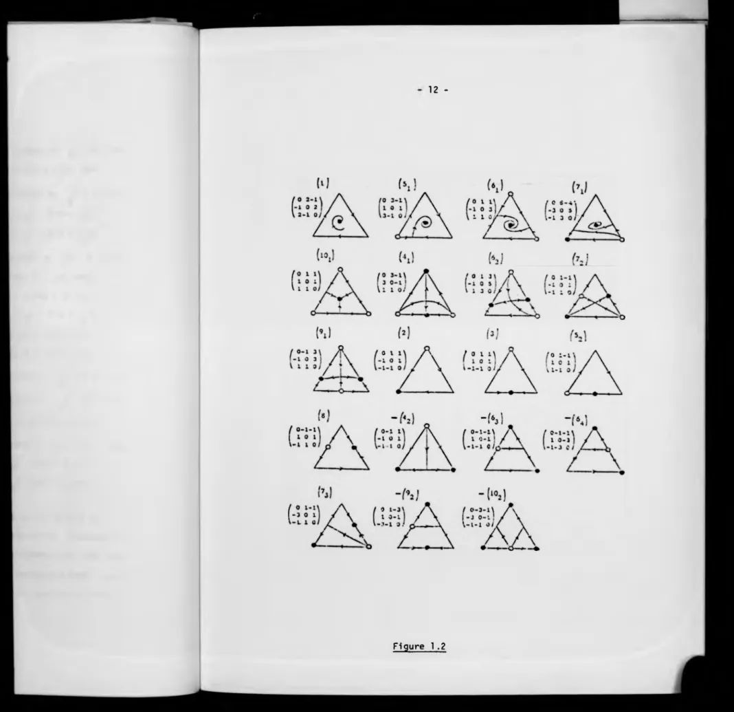
In Figure 1 .2 an example of each stable class, up to time reversal, is sketched. Attractors are marked with a solid dot, repellors by an open dot, and saddles by their insets and outsets. All other orbits
12
Chapter 2 .
Reduction of the parameter space
In this chapter we will look more closely at the parameter space
and by reducing it to a three dimensional parameter space we will study how the stable classes are joined in the parameter space, which will enable us to determine the codimension one strata in this space. The material in this chapter is based on my M.Sc. Thesis [10], where the proofs are presented in more details.
2.1 Stratification of
The decomposition of = 1R^ in Theorem 1.9 into stable classes
by the hypersurfaces (A)^. = a. • = 0 (i f j) ,
(B(A))i = -ai+1 i+2 a.+2 i+] + ai .+1 a.+] i+2 + a. i+2 a i+2 .+] = 0
(indices are mod 3) and det A = a-j2a23a32 + a13a21a32 = 0 is a stratification of Z3 i.e. a partition into finitely many smooth
disjoint submanfiolds (strata) given by algebraic equations and inequalities [ 4 ]. For convenience, we write the codimension of a matrix with respect to this stratification as cod. (In chapter 4, we
to which it belongs. However, to proceed further with the six-
dimensional parameter space and to try to partition the cod 1 stratum to its different components (strata), according to the pair of stable classes nearby, is a formidable task. Fortunately this is not needed as a further reduction of the parameter space is possible. This reduction in the next section is due to Zeeman.
2.2 The Three Torus Q
Let Q be the three torus K3/(2tiZ )3 and define
W : Q - Z3 <
a -► W(a) ♦ a = (a-| »oi2,013) « Q
j
1
0 Sin(a2 - f) Sin ajwhere W(a) = Sin dj 0 Sin(a3
1
\ Sin(a-| “ -j) Sin 012 015
-Proposition 2.1
{stable classes in Z3 > = {stable classes inlmW} 8 IR
Proof
By proposition 1.3(111), {stable classes in Z,} = {stable
+ + ->+
classes in Z3 > . But Z3 d m W 8 IR c z3 so {stable classes
+ 3+
in Z3 } = {stable classes i n l m W 8 IR } . Now lemma 1.5 implies:
3+ •>+
{stable classes i n l m W 8 IR } = {stable classes in lmW} 8 IR . □
The problem of stratification of the parameter space into stable classes therefore reduces to stratifying the set lm W or equivalently
the 3-torus Q . To do this we identify a e Q with W(a) e Z3 and thereby extend the notions of sign class, combinatorial class and stable class to Q , e.g. a e 62 means W(a) e 62 .
We start by studying the combinatorial symmetry
k " 3 “k k + i,j
1 _ 4 it . , 4IT
°1
- T ' ajand
aj T ~“i
action of n3 , the permutation group of {1,2,3} , on Q by
(ij)a = a' , i t J » where
Then it is easy to check that (1) a = a and for distinct i,j,k we
have (ijk)a = a' where • Furthermore one can show by
Q
Q
w
w
->z
3
i.e. The action of on Q gives the combinatorial symmetry of
Q . The time reversal symmetry in Q is obtained by noting that W(a+ir) = -W(a) where (a+ir).j = a^+w .
Next note that the twelve planes = 0 , j (i = 1,2,3)
3
partition Q into 4 cubic regions each of which lies in a sign class. A straightforward calculation in [ 10 ] also shows that we obtain the
/O
expression (SiWia)))^ = Sin(ai+^ - + ^-) , the simple form of
which is due to the choice of j in the definition of W .
Hence the hypersurfaces $. = 0 , 1,2,3, reduce to the planes a.j+i - a..+2 + y = 0 (mod it) , i = 1,2,3, and we can check from Theorem 1.9 that in fact only the three planes a^-j - y = 0
(i = 1,2,3) contribute to the stratification. We also observe that
the hypersurface det A = 0 reduces to the surface det W(a)=Sinc^ Sinc^Sinaj + Sin(a-| - j)Sin(a2 - j)Sin(ag - y) = 0 which in each cubic component
of C-| in Q joins three pairs of the opposite edges (Figure 2.1), and in each cubic component of C7 separates (7j) and (-7-j) from
17
Collecting all this information and using Theorem 1.9 we have deduced:
Proposition 2.2
The stratification of Q into stable classes is determined by the planes “i = 0 , , w , (i = 1,2,3) , the planes
“i “ “i+l + 1 = 0 and the surfaces det W(a) = 0 in and Cy .
□
The stratification of Q is sketched in Figures 2.3 and 2.4. These are obtained by using the algebraic conditions for the stable classes extracted from Theorem 1.9 and applied to Q by proposition 2.2. The combinatorial and time reversal symmetries of Q 4*“«. then used to complete the stratification. Figure 2.3 depicts the layer of
Q with 0 s ai s j while Figure 2.4 corresponds to y s a-| s it The other half of Q is the time reversal of this half under the relation W(a+ir) = -W(a) . For Figure 2.3 we have drawn the cross- section oj = g- and for Figure 2.4 the two sections a-j = y and <»1 = • A perpendicular arrow to the plane a^+i - a1+2 + y = 0
- 5 , ^ *> ♦ -«JL -<"* - 6 , 1
7
I !T
31
\
- V — O 3r
&
k
Qm % & _ 3X k
a
~
n
^ \ 5'
c &/
jit^ à
C/US4 10 r\ b_____________
- 19
1fV
-j
/
' 3
r
X
'
1 \
3 S,
**
6i 5.
-/ 6'
>ci \ 1
*
io, ¡io.
__ L
é. l+2
*
6,
+ i6ii
-?•
** — i6;l i. _
a
J^V
O f . r l L ÙA-OSS S t e l l o »
1 X
2
p
n
1
n
^
—
^ J > ^
3
6
, 4
3
a6,5. 5x
z
S
_
>°i/ ’
/ »C,
... .*
63
io*
A
<+.
c:
"2
63
\ \
Olòii Siiti »»\2.3 Cod 1 strata
In this section we will determine all the cod 1 strata of different types as defined in section 2.1.
Proposition 2.3
Up to time reversal, there are 38 cod 1 strata of different types.
Proof
A cod 1 matrix has at most one zero off-diagonal entry and so it 3+
must be in 1m W 8 IR . Hence {cod 1 strata in Z,} = {cod 1 strata
3+ 3+
in lm W SIR } = {cod 1 strata in 1m W} 8 1RJ . I t is then sufficient to determine the cod 1 strata in lm W or equivalently in Q . Now proposition 2. 2 implies that the cod 1 strata in Q are contained in
the planes * 0 , y , » , , the planes a. - ai +1 + ^ = 0 and in the surfaces det W(a) = 0 in C-| and in the tetrahedron in Cy . Using the three cross sections in Figures 2.3 and 2.4 we find that up to time reversal there a'-e 38 cod 1 strata, each of which lies on the
bounday of a distinct pair of stable classes. □
These 38 cod 1 strata are listed in appendix 1 according to the pair of adjacent stable classes. We have enumerated these by
38
I4 (i = 1,2,...38) so that cod 1 stratum » U I, . To fully under-
1 i=l 1
21
Chapter 3.
Local and Global Bifurcations
In this chapter we first set up the terminology in which all our results are expressed. This terminology is in line with that of Arnold for bifurcation theory in [ 4 1 and C 5 ], which we have adapted to our problem. We then look at the bifurcations induced as a smooth curve intersects a cod 1 stratum transversally and we find that locally degenerate Hopf bifurcations and exchange of stability (transcritical ) bifurcations are possible. The study of these will enable us to determine the phase portraits of the cod 1 flows i.e. those induced by cod 1 matrices.
3.1 Unfoldings and deformations
We start with some basic definitions:
Definition
A k-unfoldinq of A e is a smooth map f : U where U
k
is a neighbourhood of 0 in IR and f(0) = A . The germ of such f
at 0 is called a k-deformation of A . □
We write (U,f)k for a k-unfolding and (0,f)k for its germ.
Given a deformation (0,f)k with a representative f : U -» we
so that we are confined to an arbitrary small neighbourhood of
f(0) in . For convenience 1-unfoldings and 1-deformations
are called unfoldings and deformations, and are denoted by (U,f) and (0,f) respectively.
A deformation of A e is called transversal if it is
transversal (I) to all strata in Z^ . Hence a transversal deformation contains perturbations representing all the stable classes nearby. Clearly a deformation of a cod j matrix, 0 s j s 6 , is transversal iff it is transversal to the cod j stratum. Next we will define the notion of equivalent deformations.
Definition
Two deformations (0,f)k and (0,f)k are equivalent if for
every pair of representative unfoldings (U,f)k and (U,f)k ’ there
* -* * _*
exists U c U , U = U , a homeomorphism n : U -*■ U and a one
*
parameter family of homeomorphisms : A a , e e U , which for each e gives an equivalence between f(e) and f(n(c)) and such
that H£ depends continuously on e . □
The deformation (0,f)k is said to be induced from (O.f)^ if
1
/ nthere exists germ of contonuous maps j : R -*• IR with j (0) = 0 such that ? = foj . A deformation (0,f)k is said to be a topologically
versa! deformation of f(0) e if every deformation of f (0) is
23
-the possible deformations of that matrix. When k is minimal (0,f)k is said to be topologically miniversal and k is called the "codimension" of f(0) . Hence we have two notions of co dimension for a matrix in Z^ : one determined by its position in
the stratified and one deduced from bifurcation theory. To
avoid confusion we indicate the first notion as before by cod and the second by "codimension".
It is the object of this thesis to construct topologically versal deformations of cod 1 matrices of the planar replicator system. In fact we will prove that transversal deformations of these matrices are, in general, topologically miniversal and therefore the two notions of codimensions coincide in the codimension one case. One can also
state our result in another way and say that the cod 1 bifurcations
of the planar replicator system are stable in the sense that every
transversal deformation of a cod 1 matrix is, in general, stable with respect to the above notion of equivalence. This latter statement explains the title of the thesis.
Let us use the terminology of this section to show that all transversal deformations of cod 1 matrices in Z3 have their
representations in lm W and Q . Let (0,f) be a deformation of a
cod 1 matrix f(0) e Z^ . We can write f in the form
f (e) =
0 a12(c) a13(E )
a21(E) 0 a23(c )
a31(£ ) a32^c ) 0
0 r2(e )Sin(a2(e )- ÿ r3(e JSinajie)
f(e) = r ^ e )Sino,(e) 0 r3(e )Sin( ° > 3 ( e
)-y r] (c)Sin(a] (e )- i. CM U JSina^e) 0
where a.^ , r.. and a. are smooth germs. First we assert that
(O.f) is equivalent to (0,f) where
\
0 Sin(a2(e)- V Sina3(e)
f ( 0 = Sina^ (e ) 0
Sin(a3(e)-l Si n(a^(e )- j) Si n»2(c ) 0
This is because given any pair of representative unfoldings (U,f)
_ _
★_
and (U,f) we can choose U = U n U small enough such that
r^(e) ^ 0 for e e U , i = 1,2,3 . Then the family of diffeomorphisms
r1(e)xi
H : A -*• a with (H (x )). = --- , which by lemma 1.5 gives 1 Z r (e)x
j J J
for each e e U an equivalence between f(e) and f(e) , will depend continuously on e (here n = identity), and our assertion is proved.
- 25
respectively). Here we verify the claim for the case (ii) as the other two are entirely similar. We have (0,f) X (ei = 0} <=>
* 0 <=> 3 T T -
-* j
>|.-0
*
0
h
- «,*<'> * T>|c
0
*
0
<=> 3 T (“ i+l(e ) ' °i+2^e ^ + I^|e=0 + 0 ' The fourth inequality in the chain implies that (0,f) I (B.. = 0) while the last implies that (0,a) I ia.j+i"a^ +2 + y = 0} , proving our claim. It therefore follows that transversal deformations of cod 1 matrices in Z3 have their equivalents in lm W and Q . Based on the space Q , appendix 1 presents a transversal deformation for each of the cod 1 strata
Ij (i = 1 ... 38).
3.2 Degenerate Hopf Bifurcation
As remarked in chapter 1 the planar replicator system does not admit stable limit cycles and hence generic Hopf bifrucations which give rise to such limit cycles are excluded. However, a degenerate type of Hopf bifurcation does occur. The canonical form of this degenerate type is given by the system r = er , i = 1 , where (r,*) are polar coordinates and e is the real parameter. The phase portraits are sketched in Figure 3.1.
r
©
0 < 0 0 = 0 0 > 0
Origin is a repellor for e > 0 and an attractor for 9 < 0 . At e = 0 it is a centre and orbits are the circles r = constant. As e goes through zero the repellor is turned into an attractor, but unlike the generic case no limit cycle is born. The vector field at 6 = 0 is Hamiltonian and is highly degenerate; in fact it has infinite codimension in the space of all vector fields in the plane [ 4 ]. However such bifurcations arise in Hamiltonian dynamical systems or systems exhibiting a particular group of symmetry.
In our system, degenerate Hopf bifurcations occur in and C^ .
They were studied by Zeeman using Lyapunov functions with which the global bifurcations involved can also be understood. The results are in the following two propositions which are proved in C 25 3 for the class of central matrices. We have refined the proof in order to remove this restriction.
Proposition 3.1
A transversal deformation of a cod 1 matrix in {det = 0} in C-| induces a degenerate Hopf bifurcation.
Proof
Up to equivalence we can work in the sign class . Let (U,f)
be a representative unfolding of the deformation in question with f(e) c Sj , V e e U . Then for each e e U , adj(f(e)) has positive
entries and hence, by proposition 1.3 (ix), has a unique fixed
27
-the unfolding (U,f) for V e e U and hence assume that, up to equivalence, f has the form:
and hereafter arguments will be suppressed whenever convenient), det f(0) = 0 => e(0) = 0 and the transversality condition becomes g|- + 0 which enables us, by reducing U if necessary, to
repara-e=0
metrize the unfolding and take 0 as the parameter. We shall denote this reparametrized equivalent unfolding by (U,f) again, where f is
as above except that 0 is now the independent parameter.
_ o
Construct a Lyapunov function V. in A as follows. Let
0
X - 3A . V0 takes the maximum value of one at the barycentre E . Level curves of V„ are closed curves surrounding E .0
0
f(E) = 0(e)-a2(e) 0 0(e) + a2(e) with 0s|e(e)|<a.(e)
0(e) + a3(e) 0(e) - a3(e) 0
2
i = 1,2,3. Then det f = 20(0 +p) , where p = z a.a. > 0 . (Here i<j 1 J
where b(e) = (l ^ 0 j)-1 • Then
For 0 e U , define Vq:a -*-IR by b.(0) > 0 and z b .(0) = 1 .
1 i 1
O
Differentiating VQ along the orbits of we obtain after some work (see [25]):
Vq(x ) 9W9(x) where Wg (x)
bi ( 0)
2nx 1 z b (e)b.(e)(x.-xY
i i<j J_____ J
(z bi(6)x.)2 > 0 .
If follows that, at 0 = 0 , orbits of 6f(0) are c^ose<^ curves of V g ( x ) = constant, which fill out a . When 0 > 0 all orbits of Af(0) intersect the level curves V Q( x ) = constant transversally and hence spiral towards the maximum of VQ at E . Finally, when 9 < 0 ,
o
the reverse situation occurs and all orbits in a\E spiral outwards from E . (Figure 3.2)
Figure 3.2
Therefore a degenerate Hopf bifurcation is induced at E similar
to the canonical form of Figure 3.1. □
P ro p o sitio n 3.2
A transversal deformation of a cod 1 matrix in {det = 0}
separating ( 7 ^ and (-7^ in C? induces a degenerate Hopf bifurcation.
Proof
We will work in the sign class S7 and, by steps similar to those in the proof of proposition 3.1, we can assume that a representative unfolding (U,f) of the deformation has the form
f(e)
/ 0
e-a2(e)
e+a3( )
e + 8^ 0)
0
e - a3(e)
e - a.j(e)
e + a2( ) wi th a.j (9 ) ,a2(a ) > 0 ,
0
a,(0) < 0, 101 < | a .(o ) | and 6(0) = £ a.(9)a.(e) > 0 for 0 e U .
J 1 i<j 1 J
2
Note that in this central form 8^(0) = 0 + p(0) and hence the conditions above are equivalent to those in theorem 1.9. For V 0 e U , X1 is an attractor, X2 a repellor, X3 a saddle and E a fixed point. There is a saddle
a.(0)-e -a,(e)-0 —
2-M = (—---- , 0 , --- ) on X, X, and another
a1 (e)-a3(e)-2e a1 (0)-a3(0)-2© J
a_(e)+9 -a,(e)+0 -2—
Q0 = (0 , -i--- , --- ) on X?X
o _b - ( 0 )
Let V :A -*1R be defined by VQ(x) = (n x. 0 0 ^ 1 1 1)r b.(e)x. 1 where
b. = and b = (z 7— ) 1 are as in proposition 3.1. Here b, > 0
1 ai i ai 3
but b, b1 , b^ < 0 . VQ takes the maximum value of one at E and vanishes on the line B.C. , 0 0 where
Be ‘ (a1'c0)-a3(e) • 0 • a ^ o j - a ^ ) and Ce = (°* a2(e)-a3(0) *
-a,(0) ----
----a (9)---a (9)) • ----and on the h----alf °Pen 1ines X^X3\{X^}----and X2X3\{X2) .
The positive level curves of Vg are closed and fill the interior of the triangle XQBQC0 while the negative level curves join X-| and X2 filling the interior of the trapezium X^X2CQBg . Furthermore
V0(x) -« as X -»interior of X^X2 . (Figure 3.3)
a.(0) -a 3(0) a2(0)
Figure 3.3
Differentiating V. along orbits of A0
M 0)
f(0) we obtain
■> V x) = 0W9(x) where W0(x) = -(nxi )z ^ ( e J b j f a H x ^ X j ) .
i ^ j
o
Vq(x) = 0 ; hence orbits of 6f(Q) ’n 6 are ^eve^ curves of VQ . Note that Bq = Mg and Cq = Qq and hence the open line QqMq is an orbit which is therefore a saddle connection. Above this line orbits are closed and fill the interior of the triangle X3QqMq •
In the trapezium X2QgMgX.| orbits flow from the repel lor X2 to the attractor Xj . When e > 0 , V0 > 0 and orbits of
o
intersect level curves of VQ transversally in M E . We observe that p = I a ^ > 0 => (aj+a3)a2 > - a - ^ => a^+a3 > 0 and
similarly a2 + a3 > 0 . So it follows that
-a,(e)-e -a,(e) -a,(e)+e -a,(e)
— i-- < — £--- and — -- > —
---a1(0)-a3(e)-2e a1(9)-a3(9) a2(9)-a3(e)+2e a2(9)-a3(e)
and hence M„ lies below B_ while Qq is above C. . Therefore the
outset of Q. cannot cross B.C„ on which V„ = 0 and must go to E The inset of M0 must therefore come from X2 ; it separates the basins of attraction of E and X-j . For e < 0 , the reverse situation occurs: The inset of M„ must come from the repellor E , while the outset of Q0 goes to X-j and separates the basins of repulsion of E and X2 .
Therefore a degenerate Hopf bifurcation is induced at E and at the same time a crossing of the inset of M„ and the outset of Q.0 0
through the saddle connection QgMg takes place. □
The local and global behaviour of these bifurcations is therefore understood. We shall return to them again in chapter 6.
-3.3 Exchange of Stability Bifurcation
In this section we prove that transversal deformations of cod 1 matrices in ia^j = 0} and (e^ = 0} induce exchange of stability
(transcritical) bifurcation, when the flow is extended to a neighbourhood of a in the invariant plane l x. = 1 . The canonical form of this
i 1 bifurcation is given by the system
2
(a) x = g(x,e) = ± x ± ex
l = 0
x,e c F
Figure 3.4 gives the phase portrait when the plus signs are taken in both terms. For the flow restricted to the invariant lines
e = Constant < 0 , the point x = 0 is an attractor and x = -e is a repellor; whereas for the invariant lines e = Constant > 0 , x = 0 is a repellor and x = -e an attractor. Therefore as e goes through zero the fixed points cross each other and exchange stability.
In general consider the smooth vector field
«O' ^
j X = f(x,e)
(b) < x,e elR
1 « . 0
satisfying the conditions
b(i) f(0,0) = H (0,0) = ¿ 1 (0,0)
9x 9c
b(ii) ¿ 1 (0,0) 4 0 9X9c
92f
b(iii)
U -
(o.o)
4
o
9XThen it can be shown that (b) is locally equivalent to (a).
Conditions b(i)-b(iii) can be generalized for higher dimensions C 12 ], but then they will be tedious and non-intuitive. It is by far better to use the celebrated reduction theorem [ 4 ] [ 12 ] for reducing the vector field to the centre manifold, which we will now explain. Let
(c) x = h(x) , x e R n
[ 12 ] there exists for each r > 0 a Cr-invariant manifold tangent to EQ at origin. The reduction theorem now states that (c) is locally equivalent to the family:
.
P = hQ (p) P £ R
.
< q = -q q £ R
j r = r r £ R
where the first equation gives the dynamics on the centre manifold. In other words we can neglect eigenvalues of non-zero real part and obtain the topological picture by "suspending" the flow induced on the centre manifold.
Combining the above results, we deduce that if (c) has a two dimensional centre manifold on which the dynamics satisfies the conditions b(i)-b(iii), then (c) is locally equivalent to the system
(d)
x = ±x ± ex
e = 0
q = -q
r = r
x ,e e IR
q e IR l r £ IR
35
-portraits of the flow on three invariant planes e < 0 , e = 0 and e > 0 are sketched in Figure 3.5.
>
—4
'
'
'
f
'
1
f
4 c *
‘
i
*
JS.
>
'
>
at
V
1>
±
4C > DC
e < 0 e = 0 e > 0
Figure 3.5
In the space of one parameter family of vector fields, families like (d) which undergo exchange of stability (e is now considered as the parameter rather than a state variable) are not generic. In fact the only generic families are those undergoing Hopf bifurcation or saddle-node bifurcation C 5 3 . However exchange of stability can arise when restrictions are present as in the replicator system.
We now begin to study exchange of stability at a vertex of a In the rest of this chapter we consider the replicator equations
’ a
x = V (x) in a neighbourhood of A in the invariant plane Ex. = 1 .
Proposition 3.3
Let (0,f) be a transversal deformation of A with
f(e) =
( 0 ai2( 0 al3(E )
a2 1(e ) 0 a23(e )
U 3l(e) a32(E ) 0
where a2 1(0) = 0 and, by transversality, a ^ (0) £ 0 . Reparametrizi and taking a12 as the new parameter and using coordinates (x2,x3)
around we obtain the following autonomous system in (x2,a2 1>x3 ) :
x2 = x2^a21-al 2 ^ x? + ^a9i^®^”ai■?(®)“an (0) )x-j + h.O.tl23 13V 31
(e) <a 21 " 0
x3 = x3[a3 1(0) + h.O.t.]
where h.O.t. indicates higher order terms in x2>x3 and a ^ . As
a3l (0) 4 0 • plane x3 = 0 is the centre manifold at (0,0,0) , on which the dynamics is given by:
x2 = a2 1 x 2 ‘ ai2^°^x2 + hl0-t> < .
j^a21 = 0
It is easily seen that the conditions b(i)-b(iii) are satisfied as
b ifu rc atio n on = 0 whose suspension in the hyperbolic d irec tio n
X-jX3 gives the overall b ifu rc a tio n (see Figure 3.5 where both
a 3 l( 0 ) and a ^ ( 0 ) are assumed p o s itiv e ) . □
Figure 3.5
To deduce a sim ila r r e s u lt fo r the b ifu rc atio n at an in t e r i o r
point o f an edge we need a lemma.
Lemma 3.4 * 3
I f A e ( e i = 0} is a cod 1 matrix then det A f 0 .
Proof
3+
We can w rite A = W(o).r with o e Q and r e IR (see
proposition 2.3). Assume WLG that A e (63 = 0} ; then
“ l ”a 2 + T = ® and det w(a ) = Sin°^Sini^Sina2
+ Sin(<*i- y )S in (a2 " •j)Sin(a2~ y) = Sinfo^- yJSino^Sino^
+ Sin(a2~ -j^)Sin(a2_ jJ S in f c ^ - -j) = ) Sinfa^- -j) Cosio^-a^)
-Cos(a^-a^- -j) = Sina^Cos g- C o s g - ) =
C°s g- Sina i Sin (a2 -a3 + g) = 6-j Sina^ + 0 since W(a) is a cod 1 matrix
Proposition 3.5
A transversal deformation of a cod 1 matrix A £ {g. = 0) induces an exchange of stability bifurcation at an interior point of
Xi+lXi+2 *
Proof
Assume A e {6^ = 0} and let (U,f) be a transversal unfolding of A . Using lemma 1.5 we can further assume by multiplication with a suitable matrix and reversing time if necessary that:
0 a a1 3(e)\
f(e) = a 0 a23(e ) ! where e e U
a3l(e) a32^£ ) 0 /
and a is a positive constant. The point H = ($, J, 0) , the mid
point of ^1^2 * 1S then fixed for V e e U . Taking coordinates (x^.x-j) , the vector field around H becomes (arguments are suppressed)
i , .
, («31-» 32)x1 * ( a.3.1.- a3 r a13-a23>,3 l , h . 0 . t .
'3 ' 3 (g)
i , ■ - J X, ♦ ‘‘ » - z s - J i - a a
1
, h . o . t .39
-Furthermore, we can take the eigenvectors of the linear part of the vector field (g) at 83 = 0 as new axes and put
f a
X3 = 7 w
X] = v + (a,3(0)-a23(0)-a3 1(0)-a32(0))
J
Then (g) will be reduced to the autonomous system:
W = 2a S3W + (a3 1(0)-a32(0))vw - (det f(0))w2 + h.O.t.
< 63 = °
v = - | v + h.O.t.
The v direction (corresponding to x^ direction) is hyperbolic for V 63 e U.| . Therefore as in [ 12 ] we seek a centre manifold v = h(v,e3) tangent to (w,e3) plane at (w,e3,v) =(0,0,0) . We
therefore write
v h(w ,83) = pw^ + qwe3 + re3 + h.O.t.
where p,q and r are constants that can be determined by using the invariance of the centre manifold. But this is not necessary. Since the contribution of h to the first term in (g) gives terms of order three in w and 83 , we deduce that up to second order terms the dynamics on the centre manifold is determined by
w =
Furthermore, we can take the eigenvectors of the linear part of the vector field (g) at S3 = 0 as new axes and put
f a
x3 = 7 W
X1 = v + (a1 3(0)-a23(0)-a3 1(0)-a32(0)) J
Then (g) will be reduced to the autonomous system:
W = Ja S3W + (a31(°)-a32(°))vw " (det f <° ))w2 + h.O.t. < 63 = °
v = - | v + h.O.t.
The v direction (corresponding to x-| direction) is hyperbolic for V 63 c Uj . Therefore as in [ 12 ] we seek a centre manifold v = h(v,s3) tangent to (w,s3) plane at (w,e3,v) =(0,0,0) . We
therefore write
2 2
v = h(w ,83) = pw + qw83 + rs3 + h.O.t.
where p,q and r are constants that can be determined by using the invariance of the centre manifold. But this is not necessary. Since the contribution of h to the first term in (g) gives terms of order three in w and 83 , we deduce that up to second order terms the dynamics on the centre manifold is determined by
40
-Since, by the lemma, det f(0) + 0 we find that the conditions b(i )-b(iii) are satisfied and hence the vector field is the
suspension of a system undergoing exchange of stability bifurcation (see Figure 3.6 where we have taken det f(0) > 0) .
l
V V
B3 < 0
s3 = 0
s3 > 0
Figure 3.6
Next we prove a technical lemma which we need in later chapters. Let (U,f) be an unfolding of the cod 1 matrix f(0) e {a^. = 0} or f(0) e is. = 0} .
Lemma 3.5
Given 5 > 0 there exists a neighbourhood N of the non
hyperbolic fixed point of Af(Q) in A such that the length of arcs
of orbits of . in N is smaller than 6 for V e e U .
f ( e )
Proof
(i) Consider first the case f(0) € {a.. = 0} . Assume WLG 1 J
Nn = ^(x2*x3^ I Ix2I < 1 ♦ Ix3I < • Suppose a3 1(0) > 0 , so that the phase portraits are as in Figure 3.5. x3 is positive,
respectively negative, for points in N with positive, respectively dx.
negative, x? coordinate. Also = 1 on a cubic curve C+ which
passes through the two fixed points and is close to the hyperbola
a31 (°)x3 =
Similarly
X2^e~al 2(®)x2+(a23(0)-al3(0)-a3i(0))x3 1 in for small dx3
= -1 on a cubic curve C which passes through the t
two fixed points and is close to the hyperbola
a31 (0 ) x3 = ~x2^e "a i 2 ( ° ) x2+(a 2 3 ^ " a l 3 ^ ° ^ ' a 31 ^ ^ x3
^
’ n N- f o r smaH1
For each e e U , these two curves partition N, into five regions (three regions when e = 0) in each of which the vector field (e)
dx., dx,
satisfies either laid " 1 or laxrl ” 1 • {Figure 3'7)
J
'
4
-, . ' r
' ^ '
C v
^
^
Ì — - - *— —
t
- -
1
'
/
/C"
/
1
'
1
Figure 3.7
An orbit of in can only intersect at most once one
42
-orbit in in a region where dx3dx2 < 1 is at most
\l L
*-i
dx3x2
(gjj— ) dx2 which is therefore less than 2/2 z . Similarly
the length of an orbit in N in a region where
mos
t f
/7
J-i.
dx3
dx2 > 1 is at
dx2 2
(axj} dx3 which is again less than 2/2 z . We
conclude that the total length of an orbit in N£ is at most 4/22 and the result follows. Same argument holds when a ^ O ) < 0 .
(ii) When f(0) e {6^ = 0} we use the vector field (g) and
the proof is exactly as in (i). 0
Remark 3.7
The property in the above lemma always holds for a hyperbolic fixed point of a C^-family of planar vector fields. More precisely if x = X(x,e) is a family of vector fields with X: 1R x ]R ir a
1 2
C -map and 0 e IR a hyperbolic fixed point of x = X(x,0) , then ?
given 5 > 0 there exists a neighbourhood of 0 e IR in which the length of orbits of x = X(x,e) are smaller than S for all e with
nonhyperbolic fixed point. For example the orbits of the flow
r = -rk k 2 2
<,
.
0 = 1»»
have infinite length in any neighbourhood of origin as can easily be checked directly
,dr k .
<39 " -r => L = ds =
f ; A *
fTr,r° r1-k dr = -) . 0
U
A
♦ r ~ X dr0 >
Finally we note that the study of the cod 1 bifurcations in
43
-nonhyperbolic fixed point. For example the orbits of the flow
r = -rk k 2 2
■< 0 = 1
have infinite length in any neighbourhood of origin as can easily be checked directly
,dr k .
= "r => L = { ds = _
dr > f ° r1 Jn
0 h + r2(Ji) 2 dr
-k dr = »)
Finally we note that the study of the cod 1 bifurcations in
Chapter 4 .
Versal deformations of cod 1 matrices (Part one)
We will study topologically versal deformations of cod 1 matrices in two separate chapters. In the present we consider the cod 1 matrices satisfying the condition that no cycle of saddles appears in the flow induced by them or in the nearby stable flows. This is the case for matrices in I.. , 4 s i s 38 (see appendix 1). The remaining three cases are much harder to deal with because of
the presence of cycle of saddles. We will need some preliminary results in chapter 5 before we set to tackle these cases in chapter 6.
The results in this chapter were obtained by me independent from Peixoto's method in [ 19 ]. However in presenting them here I have modified my original version of proofs so that the reader familiar with that classic paper can follow the steps more easily.
4.1 Fundamental Domains
45
-¿A 1S partitioned into a finite number of closed domains each of which is bounded by an attractor, a repellor, a number of saddles and by saddle séparatrices and orbits in 3A . We call these
fundamental domains (F.D.) which are of five different types labelled as in Figure 4.1.
(b) (b‘ ) (C) ( C )
A
A
fl
.
>\
y
V
'f Y i’ / '\
^4
w < 1 /Figure 4.1
Consider transversal deformations of cod 1 matrices in 1^ , 4 s i s 38 . At the bifurcation point a F.D. is transformed into a F.D. except that F.D's of type (a), (b) and (c) can also shrink to the closure of union of one, two or three orbits respectively which
we denote by L1 , L2 and L3 (see Figure 4.4). The matrix of
allowed transitions between F. D. 's is given by:
(a)
/ 1 1 1 0
0
\
(b) 1 1 0 1 0 (a) <-> L1
(b1) 1 0 1 1 1 and (b) <-> L2
(c) 0 1 1 1
0 l (c) <-> L
3
( C ) 0 0 1 0 . /
attractor or the repellor, but not both, may undergo exchange of stability. If the repellor is not undergoing exchange of stability call it the base of the F.D., otherwise call the attractor the base. We note that in (c ') the repellor never undergoes exchange of stability, so it is always the base. Pick a small fixed positive number r . Take the arc, C , of the circle of radius r with the base of the F.D. as its centre and parametrize it arcwise linearly from 4> = 0 to 4> = 1 , anticlockwise if the repellor is the base, clockwise if the attractor is the base (Figure 4.2). Now define the $ coordinate of a point P in the interior of the F.D. to be the value of ♦ at which the orbit through P , aA (P) • inter sects C . The points on the left and the right boundaries of the F.D. are given the $ coordinate 0 and 1 respectively. We consider type (c*) as the limit case of Figure 4.3 for which $ is defined on both boundaries. However,in all cases, 4> remains undefined for the repellor and the attractor points.
To define the z coordinate we first need to introduce what we call an R-curve. Given two points one on each side of the boundary
47
-orbits of the F.D. with a definite ratio of arc length. We define it explicitly for type (a); it is similar in others. Let X and Y be opposite points on the boundary of a F.D. of type (a) with repellor A , attractor C and saddle B (Figure 4.4).
then the R-curve joining X and Y (always drawn by broken lines) is the curve which intersects the orbit with coordinate $ at a point
Lemma 4.1
R-curves are continuous.
Proof
As the proof is similar in F.D.'s of different type, we will give the proof only for Type (a). (Figure 4.4) All we need to check is that the length of orbits with $ $ 0 vary continuously with ♦
and that as $ 0 the length of orbits tend to t(AB) + *.(BC) . To prove the first assertion take an orbit with coordinate $q ^ 0 and choose e > 0 . By lemma 3.6 and remark 3.7 there exists neighbourhoods of A and C such that the length of orbits in each is less than ^ . Outside these neighbourhoods, the continuity of the differential
Put y =
X
fc(AY) + t(YC) t(AB) + (BC)
MAY)
MAX)
and
3
Figure 4.4
orbits of the F.D. with a definite ratio of arc length. We define it explicitly for type (a); it is similar in others. Let X and Y be opposite points on the boundary of a F.D. of type (a) with repel lor A , attractor C and saddle B (Figure 4.1).
q * (¡.(AX)
Put Y =
i(AB) + (BC)
X = J K A Y ) ^ fc(AY) + «.(YC)
Figure 4.4
then the R-curve joining X and Y (always drawn by broken lines) is the curve which intersects the orbit with coordinate $ at a point
D such that — = (1 - <j>)y + <t>x . W e must now prove: t(AD) + «.(DC)
Lemma 4.1
R-curves are continuous.
Proof
equations with respect to initial conditions [ 1 ] implies that the length of orbits with <t> sufficiently close to 4>0 differs from
that of $0 by at most ^ . Hence the total length of orbits with $ close to <f>Q differs from that of <*>0 by at most e and the assertion follows. The second assertion is proved similarly by
considering, in addition to the two neighbourhoods around A and C , a neighbourhood around C in which length of orbits remain small. □
Let (U,f) be a transversal unfolding of f(0) e I. , 4 s i s 38 We now proceed to partition the fundamental domains in Af(e ) • e e U , by R-curves as follows.
Step 1
Start with the F.D.'s of type (a), (b) and (c) which shrink to
1 2 3
L , L and L respectively. Through each saddle take the R-curve joining it to the point on the opposite side of the boundary which lengthwise divides the boundary of that side in the same ratio as the saddle divides its own side of the boundary. (Figure 4.4)
(a) <-> L1 (b) <-> L2 (c) <-> L3
Figure 4.4 Step 2
F.D.'s : If the saddle is undergoing exchange of stability with the repel lor (attractor) of the F.D., choose the opposite point to be at
the same distance on the boundary to the repel lor (attractor) as the saddle is to the repellor (attractor). In other cases, take the R-curve from the saddle to the point on the opposite side which is the endpoint of an R-curve determined by step 1 in a neighbouring
F.D., or, if such a point does not exist, to the saddle on the opposite side, or, if neither of these points exist, to the point on the opposite side with the same dividing ratio of the boundary as in step 1. Figure 4.5 illustrates examples of these cases.
from the endpoints of the R-curve(s) determined in the two steps above to similar endpoint(s) on the opposite side or, in the absence of such endpoint(s), to the point(s) with the same dividing ratio of the boundary.
The complete result is given in appendix 1. The partition of
Af(e) ’ e e u • obtained in this way consists of a number of sub- domains in each F.D. ; a sub-domain is either triangular i.e. bounded
(a) <-> (b) (b) <-> (c) Figure 4.5
(b) <-> (c)
Step 3
50
-by a repel lor (an attractor), two semi-orbits flowing from the repel lor (flowing to the attractor) and an R-curve, or rectangular i.e. bounded by two orbit segments and two R-curves. (Figure 4.6)
Figure 4.6
Now let M be a point on an orbit AB in a sub-domain of a F.D. with, say, A between M and the base of the F.D. We define the
z coordinate of M to be ^ .
*(AB)
Therefore, given e e U , any point M e a lies in a sub-domain of a F.D. in and has accordingly a pair of (<t>,z) coordinates with 0 s <j> s 1 and 0 s z s 1 . Points which lie on the boundary of
two or more sub-domains will have accordingly different coordinates with respect to the sub-domains in question. For simplicity we will not refer explicitly to any particular sub-domain and always assume that (<}>,z) refers to the coordinates of M with respect to a given sub-domain of A,, . .
f ( e )
4.2 The Family of Homeomorphisms