kth order Markov extremal models for assessing heatwave risks

(will be inserted by the editor)

k

th-order Markov extremal models for assessing

heatwave risks

Hugo C. Winter · Jonathan A. Tawn

Received: date / Accepted: date

Abstract Heatwaves are defined as a set of hot days and nights that cause a marked short-term increase in mortality. Obtaining accurate estimates of the probability of an event lasting many days is important. Previous studies of tem-poral dependence of extremes have assumed either a first-order Markov model or a particularly strong form of extremal dependence, known as asymptotic de-pendence. Neither of these assumptions is appropriate for the heatwaves that we observe for our data. A first-order Markov assumption does not capture whether the previous temperature values have been increasing or decreasing and asymptotic dependence does not allow for asymptotic independence, a broad class of extremal dependence exhibited by many processes including all non-trivial Gaussian processes. This paper provides akth-order Markov model framework that can encompass both asymptotic dependence and asymptotic independence structures. It uses a conditional approach developed for mul-tivariate extremes coupled with copula methods for time series. We provide novel methods for the selection of the order of the Markov process that are based upon only the structure of the extreme events. Under this new frame-work, the observed daily maximum temperatures at Orleans, in central France, are found to be well modelled by an asymptotically independent third-order extremal Markov model. We estimate extremal quantities, such as the prob-ability of a heatwave event lasting as long as the devastating European 2003 heatwave event. Critically our method enables the first reliable assessment of the sensitivity of such estimates to the choice of the order of the Markov process.

H.C. Winter, J.A. Tawn

Department of Mathematics and Statistics, Lancaster University, Lancaster, LA1 4YF, U.K.

Present address:of H.C. Winter

Keywords asymptotic independence · conditional extremes · extremal dependence·heatwaves· Markov chain· time-series extremes

1 Introduction

Many devastating natural hazards are caused by events that are extreme and rare. Extreme value theory provides a general framework for modelling such extreme values. In many situations a singular extreme observation does not have a great effect, whereas combinations and runs of extreme values can cause widespread devastation. A heatwave is defined as a set of consecutive days and/or nights that lead to an increase in mortality. So when estimating risks attributed to heatwaves we need to account for the fact that one very hot day may not cause a large increase in mortality whereas a run of consec-utive less hot days can be far more damaging. Therefore any extreme value model utilised to help assess the risk of heatwaves must be able to model such behaviour reliably. In the terminology of extreme value theory, this requires a model that can capture the extremal temporal dependence structure along-side marginal tail characteristics. The data that we will model in this paper relates to summer daily maximum temperatures from a single site observed over a number of years. Therefore we want to model the extreme events of a univariate stationary series.

Let{Yt}be a stationary time-series with upper endpointyF. We are interested

in modelling the behaviour for{Yt}above some high thresholduY. Following

copula time series methods (Joe 1997), our approach is to separately model the margins and dependence structure of{Yt}. The most common approach to modelling the marginal distributions of extreme values is to fit a generalized Pareto distribution (GPD) to exceedances ofuY. The GPD takes the form

P(Yt−uY > y|Yt> uY) =

1 + ξy

σu_Y

−1/ξ

+

for y≥0, (1)

where c+ = max(c,0), σuY >0 and ξ ∈ R are the scale and shape

param-eters of the GPD respectively (Coles 2001), with the scale parameter being threshold dependent. The justification for this model is an asymptotic result of Pickands (1971) that showed that, under weak conditions on Yt, the

dis-tribution of suitably scaled exceedances of a threshold byYtconverges to the

GPD as the threshold tends to the upper endpointyF. Thus the GPD model in

equation (1) assumes that the limiting result holds exactly for a large enough thresholduY.

where within each cluster groups of dependent exceedances occur and between clusters values are treated as independent. Clusters are not necessarily consec-utive exceedances, in fact the most popular technique for cluster identification is the runs method (Smith and Weissman 1994), with run lengthl, which takes a cluster to be exceedances of uY that are not separated by a run of l

con-secutive non-exceedances ofuY. The value of l can be selected automatically

using methods of Ferro and Segers (2003). The number of clusters is Poisson distributed (Davison and Smith 1990). We wish to accurately model the tem-poral dependence of the within cluster values, i.e., the local time-series during an extreme event. Empirical distributions of cluster functionals could be used for inference of within cluster behaviour, but they have major limitations for extrapolation and so are only really suitable for model checking. Our approach is to use akth-order Markov chain for{Yt}, using only values ofYtwithin lag

kof an exceedance ofuY. We term such a model an extremal Markov chain.

Many different approaches exist for modelling the multivariate dependence structure of extreme values. First, consider two random variables (Y0,Yτ) at a time lagτ. A key way to discriminate between approaches is through the lag

τ extremal dependence measureχτ, often termed the tail coefficient, where

χτ = lim

y→yF

P(Yτ> y|Y0> y). (2)

When χτ > 0, i.e., the largest values of the variables can occur together,

the pair are termed asymptotically dependent. Asymptotic dependence arises when the conditions for multivariate regular variation hold and for max-stable distributions/processes; see de Haan and Ferreira (2006), Resnick (1987) and Davison et al (2012). Whenχτ = 0, i.e., the largest values of the variables can-not occur together, the pair are termed asymptotically independent. Asymp-totic independence arises for all non-trivial Gaussian processes and for a broad range of examples identified by Ledford and Tawn (1997) and Heffernan (2000). The conditional extremes approach of Heffernan and Tawn (2004) currently is the only model that has the flexibility to capture both of these extremal dependence classes whilst being generalisable to higher-dimensional problems. We shall base our inference on this class.

Markov processes have been assumed. After marginal preprocessing, Dupuis (2012) models heatwaves using an asymptotically independent AR(8) model. However this model is fitted to the whole series, not simply the extremes, so may lead to bias when applied to the extremes. Bortot and Tawn (1998) use theory from Ledford and Tawn (1997) to derive a class of models for first-order Markov chains that permits both asymptotic independence and asymptotic de-pendence. However these models are only justified when consecutive values are large, i.e.,Yt> uY andYt+1> uY, which is restrictive for our application.

Winter and Tawn (2016) built a first-order Markov approach, based upon the conditional extremes approach of Heffernan and Tawn (2004), that can account for both asymptotic dependence and asymptotic independence and applies if at least one component of (Yt, Yt+1) is greater than uY. The limit theory for this model has been studied by Papastathopoulos et al (2017). They find the limiting joint behaviour of (Yt+1, . . . , Yt+m)|Yt > uY, after suitable

normalisation, as uY → yF, for any integerm ≥1. For the daily maximum temperature data that are analysed in our paper, Winter and Tawn (2016) found that standard time series diagnostics, e.g., PACF and a comparison of observed and modelled cluster functionals, suggest that the first-order Markov assumption was reasonable. However, the physical mechanisms of heatwaves suggest that this is perhaps an oversimplification that could lead to an under-estimation of the risk of a heatwave event. They also found strong evidence of asymptotic independence, with significant positive dependence, and that falsely assuming a first-order Markov model with asymptotic dependence leads to overestimation of heatwave characteristics. This paper seeks to take advan-tage of the higher-order structure of the extreme values of the process through akth-order Markov model for extremes to provide more accurate estimates of the risk of a heatwave event.

Section 2 sets out the copula formulation for kth-order stationary Markov chains, with the asymptotic representations for these processes when in ex-treme states being identified in Section 3. Our asymptotically justified model forkth-order chains is set out in Section 4 and the inference for this is discussed in Section 5. A discussion of diagnostic methods for the choice of the order of the extremal Markov process is given in Section 6. Section 7 gives results for our temperature data set, from Orleans in central France, and includes com-parisons with the results of Winter and Tawn (2016) for a first order Markov model. Discussion and conclusions are presented in Section 8.

2 Copula formulations for stationary Markov processes

We shall model the stationary time-series {Yt} by a kth-order Markov chain using copula time series methods. Under the assumption that a stationary time-series{Yt}follows akth-order Markov process, the joint density function

f1:n ofY1:n= (Y1, . . . , Yn) can be written as

f1:n(y1:n) =f1:k(y1:k) n−k

Y

t=1

fk+1|1:k(yt+k |yt:t+k−1),

wherefk+1|1:k(· | ·) is the conditional density function ofYk+1|Y1:k. Here and

throughout we subscript densities and vector variables to denote the associated indices of {Yt}. We also use the notation i :j to denote (i, i+ 1, . . . , j). For stationarity the joint densityf1:k+1(y1:k+1) must satisfy the property that its m-dimensional joint margins satisfy the condition

fi1,...,im(y1:m) =fi1+τ,...,im+τ(y1:m), (3)

for all m < k+ 1, τ ∈ _N, ij ∈ N for j = 1, . . . , m, with 1 ≤ i1 < . . . <

im+τ≤k+ 1 andy1:m∈Rm(Joe 1997). As a consequence of condition (3)

the marginsfi must be identical and we subsequently denote them byf. Ad-ditional dependence conditions must also hold, e.g., (Yi, Yj) and (Yi+τ, Yj+τ)

have identical joint distributions.

We shall adopt a copula framework for modellingf1:k+1, with associated joint

distribution functionF1:k+1satisfying

F1:k+1(y1:k+1) =C(FY(y1), . . . , FY(yk+1))

=CX(F_X−1{FY(y1)}, . . . , F_X−1{FY(yk+1)}), (4)

where C is a copula with uniform margins and CX _{is the associated joint}

stationarity conditions (3) that are required forf1:k+1. Specifically, forCX we

require that itsm-dimensional marginalC_i1,...,iX _m satisfies

C_i1,...,iX _m(x1:m) =Ci1X+τ,...,im+τ(x1:m), (5)

for allm < k+ 1,τ∈_N,ij∈_Nforj= 1, . . . , m, with 1≤i1< . . . < im+τ≤

k+ 1 andx1:m∈Rm.

The reason for considering the joint distributionsCX _{with non-uniform}

iden-tical margins, instead of copulas with uniform margins, is that the extremal properties are more simply expressed for some non-uniform marginal choices. The most convenient choice of FX depends on the context: the Fr´echet or Pareto distributions are typically assumed for max-stable distributions; for conditional extremes Heffernan and Tawn (2004) use Gumbel margins; whereas for joint tail modelling Wadsworth and Tawn (2013) used exponential mar-gins. Keef et al (2013) showed that a more comprehensive approach arises for Laplace margins with

FX(x) =

(₁

2exp(x), x <0, 1−1

2exp(−x), x≥0.

Trivially, if{Yt} is a stationary kth-order Markov chain, then{Xt}, defined by

Xt= (

log{2F(Yt)} if F(Yt)<1/2,

−log{2 [1−F(Yt)]} if F(Yt)≥1/2,

is a stationarykth-order Markov chain with Laplace margins. With this for-mulation it follows that the likelihood is

f1:n(y1:n) =f1:k(y1:k) n−k

Y

t=1

cX_1:k+1(xt:t+k) cX

1:k(xt:t+k−1)

f(yt+k) fX(FX−1(FY(yt+k)))

, (6)

wherecX

1:k+1 andc

X

1:k are the copula densities for Xt:t+k andXt:t+k−1 respec-tively and xt =FX−1{FY(yt)} for all t. Here cX1:k+1 satisfies the joint density condition that arises from the stationary copula condition (5). Note that the term in the product of the likelihood factorises into separate terms for the marginal and dependence structure of the time series.

3 Asymptotic representations for stationary extremal Markov chains

3.1 Preliminaries

events as we don’t want the dependence structure of the body of the process to influence the fitting of the model to the extreme events. In particular we do this by defining an extreme event to be when the first component of the vector Yt:t+k is extreme, i.e., Yt > uE, where uE is a high threshold. Here uE is not necessarily equal to the marginal modelling threshold uY, defined

in Section 1, as it is a dependence structure definition of an extreme which can differ from a marginal definition as the rate of convergence to the limiting form can be different for these two characteristics.

So we only model the conditional distribution Yt+k|Yt:t+k−1 parametrically whenYt> uE, and we model this conditional distribution non-parametrically when Yt ≤ uE. Equivalently, this corresponds to modelling Xt+k|Xt:t+k−1 when Xt > u, where u = F_X−1(FY(uE)). Similarly, marginally we model the distribution FY parametrically for Yt > uY and non-parametrically for

Yt ≤ uY. If we use the copula formulation (4) then for large n, the likeli-hood (6) for our model simplifies to

f1:n(y1:n)≈

Y

t:xt>u

cX_1:k+1(xt:t+k) cX

1:k(xt:t+k−1)

Y

t:yt>uY

f(yt), (7)

as the terms that have been dropped contribute little or nothing to the like-lihood for the extreme value model. Details of the marginal model for FY, that is required for the second product in this likelihood, are given in Sec-tion 4.1. The first term requires the condiSec-tional distribuSec-tion ofXt+k |Xt:t+k−1 when Xt > u. Section 3.2 presents our main method for modelling extremal dependence based upon the conditional approach outlined in Heffernan and Tawn (2004). However, this model gives a limiting representation only for

Xt+1:t+k|(Xt> u) asu→ ∞. Therefore we propose an extension to give the

behaviour of the distribution ofXt+k|Xt:t+k−1 whenXt> uforu→ ∞.

3.2 Asymptotics for conditional extremes

Heffernan and Tawn (2004) propose an asymptotically justified conditional multivariate extremes approach for modelling the extremes of a vectorXt:t+m,

for any integer m >0, with all variables having Laplace margins and a joint density. We present that model and then discuss the additional conditions re-quired for{Xt}to be a stationarykth-order Markov process. Throughout the

rest of the paper all vector calculations are to be interpreted componentwise.

To explore the conditional distribution P{Xt+1:t+m≤x|Xt> u} for large uwe use an asymptotically justified form for this distribution as u→ ∞. If

x is fixed, in general the limit distribution will be a degenerate distribution. Hence Xt+1:t+m needs to be normalised appropriately so that the limiting

oru. For statistical purposes it is most simple to use the approach of Heffernan and Tawn (2004) and to normalise byXt, so that is the approach that we will take.

Heffernan and Tawn (2004) assume that there exist functions a: _R → Rm

andb: _R→Rm+, such that

P Xt+1:t+m−a(Xt)

b(Xt)

≤z1:m, Xt−u > x

Xt> u

!

→G1:m(z1:m) exp(−x),

(8)

as u→ ∞ with z1:m∈ Rm, where G1:m is a joint distribution function that

is non-degenerate in each margin, i.e., for j= 1, . . . , m thejth margin Gj of

G1:mis non-degenerate. There is no finite parametric form forG1:m.

Under weak assumptions on the joint distribution of Xt:t+m, Heffernan and

Resnick (2007) show that componentwise aand b must be regularly varying functions satisfying certain constraints, which for Laplace margins corresponds to each of the components ofa (respectivelyb) being regularly varying func-tions of index 1 (respectively less than 1). Within this structure Heffernan and Tawn (2004) found that a simple form foraandbholds for a very broad range of copulas. In particular, they assume that

a(Xt) =α1:mXtandb(Xt) =X

β_1:m

t (9)

where α1:m= (α1, . . . , αm)∈[−1,1]mand β1:m= (β1, . . . , βm)∈(−∞,1)m. This canonical parametric subfamily of aand b provides a parsimonious yet flexible family for statistical modelling.

A key property of the limit (8) is that the limiting distribution factorises, corresponding to large values of Xt being independent of the associated nor-malised Xt+1:t+m. Here, stationarity of {Xt} ensures that α1:m, β1:m and G1:mdo not depend ont. Whenβi<0 thenXt+iis asymptotically a multiple

ofXtfor all Xt> uas u→ ∞. As this deterministic structure is unlikely to occur in practice, we take a pragmatic approach and restrict the parameter space forβ_1:mso that (β1, . . . , βm)∈[0,1)m.

Different types of extremal dependence lead to different values of the extremal dependence parameters α1:m and β1:m. For 1 ≤ j ≤ m, when αj = 1 and βj = 0 the variables (Xt,Xt+j) are asymptotically dependent and are

asymp-totically independent whenαj<1. Within the asymptotic independence case a further resolution of the dependence structure is possible with 0< αj <1 or αj = 0 and βj > 0 corresponding to positive dependence; independence when αj =βj = 0 andGj is the Laplace distribution function; and negative dependence when−1≤αj<0. For more information see Keef et al (2013).

appear to impose any further constraints on the α1:k, β1:k and G1:k, when k is the order of the Markov process in expression (8), for k ≤ m. We have explored a range of examples that seem to support this. The reason for this freedom appears to be that we are not looking at the whole copula but at a slice with largeXt. Based on these empirical findings, we conjecture that there

is no relationship between these features and so in our model these features are unconstrained. In contrast the values of αk+1:m, and βk+1:m and joint

distribution functionGk+1:m, for any m≥k+ 1, do have structure imposed

by the stationary Markov behaviour and are determined entirely byα1:k,β1:k

andG1:k.

For stationary kth-order Markov chains with k > 1 no theoretical results are published other than for asymptotically dependent processes (Yun 2000). However for asymptotically dependent and asymptotically independent sta-tionary first-order Markov processes, k = 1, Papastathopoulos et al (2017) derive two possible forms forα2:m,β2:mandG1:mfor allm≥2 depending on

the value ofα1. Specifically, when if 0< α1≤1 then, for 2≤τ ≤m,ατ =ατ1,

βτ =β1 and whereG1:τ is the joint distribution ofZ1:τ where

Zj =

j

X

i=1

ατ₁−i+iβ1Z1,i forj= 1, . . . , τ,

whereZ1,iare independent and identically distributed overi, with distribution

functionG1. Note that the situation whereα1= 1 andβ1= 0, i.e., asymptotic dependence at lag one leads to asymptotic dependence at all lags, and that {Zτ}is a random walk, thus giving the results of Smith (1992). Alternatively, whenα1= 0 and 0≤β1<1, they find that, for 2≤τ≤m,ατ = 0,βτ=β1τ withG1:τ the joint distribution of

Zj =

j

Y

i=1 (Z1,i)β

i−1

1 _{forj= 1, . . . , τ,}

with Z1,i≥0 being independent and identically distributed overi, with

dis-tribution functionG1. These results prove helpful in Section 6 for developing tests for the process being a first, or higher, order extremal Markov chain.

Finally note that a kth-order Markov process can behave as a Markov pro-cess with orderkE, withkE≤k, in its extremes. In this case the information

in expression (8) for m = kE is only required to determine αkE+1:m, and

β_kE+1:m and joint distribution functionGk_E+1:m for anym > kE. The

situ-ation kE < k arises for akth-order Markov process when (αkE+1:k,βkE+1:k)

are determined by (α1:kE,β1:kE) and G1:k factorises into G1:kE and GkE:k,

4 Models for conditional extremes

4.1 Marginal modelling

As{Yt} is a stationary series the marginal distributionsFY are identical. As

discussed in Section 1, there is an asymptotic justification for modelling the marginal excesses of uY by Yt as following a GPD with distribution func-tion (1). But we do not specify a parametric form for the distribufunc-tion of Yt

belowuY. Following Coles and Tawn (1991) we model the marginal distribu-tion ofYt as

FY(y) =  



1−[1−F˜(uY)]1 +ξy−uY

σ_uY

−1/ξ

+

, y > uY,

˜

F(y), y≤uY,

where ˜F(y) is the empirical marginal distribution function ofY1:n.

4.2 Temporal dependence modelling

The limiting form of the conditional distribution (8) motivates our asymptoti-cally justified model for the conditional distribution ofXt+1:t+k givenXt> u

for a large fixed value u, and k the order of the extremal Markov process. Specifically, we assume that the limiting form (8) holds exactly for all values ofXt> uwithm=k, that the normalising functionsaandbcan be given by forms (9), and thatXt:t+k has a density. It follows that we have

Xt+1:t+k|(Xt> u) =α1:kXt+X

β_1:k

t Z1:k, (10) forα1:k ∈[−1,1]k,β1:k ∈[0,1)k andZ1:k is a random variable, independent

of t andXt, with distribution function G1:k and joint densityg1:k. Trivially,

model (10) satisfies the limiting property (8) asZ1:k andXtare independent

and exceedances of uY > 0 are unit exponential. The recurrence

relation-ship (10) cannot be interpreted as holding for all Xt, as it only applies for Xt> u. As such, series generated under this process (like tail chains in Smith

(1992) and Papastathopoulos et al (2017)) have negative drifts that ensure the process returns from an extreme state to the body of the distribution.

We need an asymptotically motivated model forXt+k |Xt:t+k−1whenXt> u. As no formal limiting results exist our approach provides a heuristic approach which provides a flexible modelling framework. By assuming that model (10) holds exactly forXt=xt> uit follows that

Xt+k|(Xt:t+k−1=xt:t+k−1) =αkXt+XtβkZk|1:k−1, (11) where Zk|1:k−1 is a random variable with the same distribution as the condi-tional distribution ofZk given that

Z1:k−1=

x1:k−1−α1:kxt xβ1:k

t

This conditional variableZk|Z1:k−1=z1:k−1has distribution function

Gk|1:k−1(z|z1:k−1) = Z z

−∞

gk|1:k−1(s|z1:k−1)ds,

wheregk|1:k−1(· |z1:k−1) is the associated conditional density function, given by g1:k(z1:k−1,·)/g1:k−1(z1:k−1). It follows iteratively that for j = 1, . . . that

Xt+k+j|(Xt:t+k+j−1 = xt:t+k+j−1) is also given by expression (11).

Conse-quently we can simulate the values ofXt+k+j, for 1≤j ≤m, without

explic-itly evaluatingαk+1:m,βk+1:mandGk+1:m.

As this is a statistical model developed based on heuristic arguments it may not give a structure that is consistent with the limiting tail chain of thek th-order process, but what is critical here is that it gives a flexible and parsi-monious statistical model for capturing the dependence of the process over a high threshold. Section 7 presents evidence that supports our statistical model through the realistic realisations of extreme events that it generates.

5 Inference

5.1 Inference for model parameters

Here we assume that the process is a stationary kth-order extremal Markov process, with k known. The estimation ofk is discussed in Section 6. Under this assumption we estimate the extremal marginal parameters (σu_Y, ξ), the extremal dependence parameters (α1:k,β1:k) and the distribution Gk|1:k−1.

Our approach is a pseudo maximum likelihood inference scheme with block bootstrap methods for obtaining confidence intervals. Specifically, we use step-wise inference, with marginal parameters estimated first, then the dependence parameters, and thenGk|1:k−1is estimated non-parametrically. This approach to separate inference for marginal and dependence structure is standard in copula modelling and has been shown to not lose much efficiency; see Genest et al (1995) and Liang and Self (1996).

From likelihood (7) our approach corresponds to standard maximum likeli-hood estimation for (σu_Y, ξ) using all the threshold exceedances of uY by {Yt}. Likelihood (7) then simplifies down to a product over the density con-tributions forXt+k|Xt:t+k−1 whenXt> u. Since G1:k and its marginals do

not take any finite parametric form, we make a temporary working assump-tion that Z1:k are independent Gaussian variables with Zj ∼ N(µj, γj2) for j= 1, . . . , k (Keef et al 2013). Under this assumption

Xt+j | {Xt=x} ∼N αjx+µjxβj, γj2x

2βj

where j = 1, . . . , k for all t with Xt > u. If we denote the corresponding Gaussian likelihood byLj, for j= 1, . . . , k, then the overall likelihood is

L(α1:k,β1:k,µ1:k,γ1:k) = k

Y

j=1

Lj(αj, βj, µj, γj), (13)

due to the independence assumption. Maximisation of likelihoodLgives esti-mates ( ˆα1:k,βˆ1:k,µˆ1:k,γˆ1:k). Unless there are constraints on the parameters

across lags then in practice these values can be most easily be obtained through maximising Lj separately for each j. Although it may appear that ignoring the dependence of Z1:k would bias the inference forα1:k and β1:k, standard

regression results show this is not the case. Furthermore, Lugrin et al (2016) find that estimating ( ˆα1:k,βˆ1:k) while accounting for the dependence inZ1:k,

through a Bayesian non-parametric estimate ofG1:k, gives only small

improve-ments relative to our much simpler approach.

At this stage the Gaussian assumption is discarded and a non-parametric estimate of the conditional distribution functionGk|1:k−1is formed. This step accounts for the dependence ofZ1:kin the subsequent inference. Our approach

to estimating Gk|1:k−1 is to obtain an estimate of the joint density function

g1:k and use this to derive the conditional distribution. For this purpose we

use kernel density estimation, similar to Papastathopoulos and Tawn (2013). Under model (10) we have that Zt+1:t+k ∼ G1:k for all t with Xt > u. We

first derive an estimated identically distributed sample ˆz(_1:i)_k, i= 1, . . . , nufrom

Z1:k, where nu is the number of exceedances by {Yt} of uE. Specifically, let t1, . . . , tnu be the indices of t = 1, . . . , n where xt > u. By inverting

equa-tion (10) we have fori= 1, . . . , nu

ˆ

z_1:(i)_k =xti+1:ti+k−αˆ1:kxti−µˆ1:k(xti)

ˆ

β_1:k

ˆ

γ_1:k(xti)

ˆ

β_1:k . (14)

For eachj = 1, . . . , k, the sample ˆzj= (ˆz

(i)

j , i= 1, . . . , nu) has zero mean and

unit variance.

Based on the ˆz1:k data, we estimate the joint densityg1:k using a multivariate

kernel density estimation methods, i.e.,

˜

g1:k(z) =

1

nu nu

X

i=1

KH

z−ˆz(_1:i)_k, (15)

whereKHis the independent multivariate Gaussian kernel function, withH=

(h1, . . . , hk) the vector of the marginal bandwidths. It follows that our estimate

of the conditional distribution functionGk|1:k−1 is

ˆ

Gk|1:k−1(z|z1:k−1) =

nu

X

i=1

wiΦ z−zˆ

(i)

k hk

!

where the weights

wi=

k−1 Y

j=1

φ zj−zˆ

(i)

j hj

! , nu

X

r=1

k−1 Y

j=1

φ zj−zˆ

(r)

j hj

!

i= 1, . . . , nu, (16)

satisfy 0≤wi≤1,P nu

i=1wi= 1, and where φis the standard normal density.

5.2 Inference for cluster functionals

From the estimates of the model parameters we can derive estimates of inter-esting cluster functionals by using the estimated model to repeatedly simulate the within cluster behaviour of the process. Our strategy for generating within cluster behaviour is to use the properties of the tail chain, where a tail chain describes the nature of the Markov chain after an extreme observation, ex-pressed in the limit as the observation tends to the upper endpoint of the marginal distribution; see Rootz´en (1988), Smith (1992), Smith et al (1997), Yun (2000) and Drees et al (2015).

Tail chains were originally developed for asymptotically dependent processes, where for Laplace margins, they correspond to the limiting process of {Xt−

u;t = 0,1, . . .}|X0 > u as u → ∞. Normalisation of Xt by a subtraction of u leads to non-degeneracy for asymptotic dependence. Denote the limit-ing tail chain by {X_t+;t = 0,1, . . .}. It follows that X₀+ follows an standard Exponential distribution and subsequent values that exceed 0 contribute to the limiting cluster. This tail chain is used to approximate the behaviour of the asymptotically dependent processes during extreme events which exceed a high thresholdv, giving the approximation for{Xt}, subject toX0> v, being provided{X_t(v):=v+X_t+;t= 0,1, . . .}. In essence the tail chain is assumed to hold exactly overv. The tail chain has a negative drift and so after sufficient steps no further exceedances ofv are possible within the cluster.

Kulik and Soulier (2015) and Papastathopoulos et al (2017) consider tail chains for first-order asymptotically independent processes. Normalising using a sub-traction ofuleads to degeneracy in this case, and less powerful location-scale norming is required. In fact for kth-order Markov chains with Laplace mar-gins, the required normalisations under the Heffernan and Tawn (2004) model formulation are given by the results in Section 4.2, with both location and scaling required.

To be precise we now set out how to simulate from the kth-order tail chain approximation above threshold v. The tail chain {Xt(v);t = 0,1, . . .}, is

sim-ulated in three steps. First the initial exceedance, X₀(v), of v is simulated as

are generated jointly, conditional onX₀(v), as

X(_1:v_k)₋₁= ˆα1:k−1X (v) 0 +

X₀(v)

ˆ

β_1:k−1

Z1:k−1, (17) whereZ1:k−1is sampled independently from ˆg1:k−1, the marginal of ˆg1:k given

by equation (15). At all subsequent time-stepsj ≥k, the transition kernel of the tail chain is used, i.e.,

X_j(v)=αkX

(v)

j−k+

X_j(₋v)_k βk

Zj|j−k+1:j−1, (18)

where theZj|j−k+1:j−1values are sampled independently from ˆGk|1:k−1. The final stage is to transform the simulated tail chain back to the original mar-gins, i.e., Y_t(v)=F_Y−1(FX(X_t(v))) fort= 0,1, . . ., and so when X_t(v)> uthen

Y_t(v)> uY.

The justification for the use of the asymptotically motivated transition ker-nel (18) is thatX_j(v₋)_k> u. WhenX_j(v₋)_k< uthe algorithm can still be used but

the quality of the approximation is likely to become poor the further X_j(₋v)_k

drops belowu. WhenX_j(v₋)_k <0 the transition (18) cannot be used asβk <1

and so the tail chain is immediately terminated before generating X_j(v). This

is not restrictive as X_j(v₋)_k < 0 corresponds to the process falling below the median and so it is reasonable to treat the extreme event as having finished. The tail chain is run untilX_j(v)is small enough that there is a negligible prob-ability of obtaining a further exceedance ofv. In practice it is most simple to run the chain for a fixed long timem, with m= 40 found to be sufficient for our examples in Section 7.

For first-order processes, Winter and Tawn (2016) showed that it is equally easy to simulate the tail chain forwards and backwards from a cluster maxi-mumM, given that M > v, or to simulate an arbitrary exceedance of v and simulate forwards only. Forkth-order tail chains it is more computationally ef-ficient to use the latter approach since it requires only forward simulation and does not require the initial simulated value to be the cluster maximum, which would lead to the simulation scheme requiring rejection methods to ensure this property. As all the cluster functionals that we are interested in can be evaluated using only forwards simulation we restrict attention to this approach.

There are a range of cluster functionals that we are interested in estimat-ing. The extremal dependence measure χτ, defined by expression (2), is not

helpful as for all processes that are asymptotically independent at lagτ then

χτ = 0. However the sub-asymptotic extremal dependence measure χτ(v) for τ= 1,2, . . ., i.e.,

whereyv=F_Y−1(FX(v)), provides a helpful summary of the level of dependence in the tail. This can be evaluated as the proportion of tail chains which are above the thresholdj steps after an exceedance. We are also interested in the distributionπ(i, v) ofDv, the number of exceedances ofv, in a cluster. To be precise

Dv=X

t∈C

I(Xt−v)+,

where _I(.) is the indicator function and C is a set of values constituting a cluster and π(i, v) = P(Dv =i | Dv >0). Furthermore we use the notation

Π(i, v) = P(Dv ≥i| Dv >0) to denote the probability of a cluster abovev

with at leastiexceedances.

The mean of the cluster size distributionπ(·, v) is the most widely used cluster functional of the extremes in a time-series at a levelv, i.e.,

∞

X

i=1

iπ(i, v) =θ(v)−1, (20)

which is given by the reciprocal of the sub-asymptotic extremal indexθ(v) (Led-ford and Tawn 2003), withθ(v)∈[0,1]. See Winter and Tawn (2016) for details of how to use the forward tail chain for estimating these functionals.

When reporting results it is more instructive to give estimates of the proba-bility of a cluster functional value occurring within a given time period rather than in a single event. To make such a conversion we need to account for there being a Poisson, meanψv, number of independent and identically distributed clusters of the levelv in the time period, where forv≥u

ψv=θ(v)[1−F˜(u)]nT

1 +ξ

_v−u

σu

−1/ξ

+

,

wherenT is the number of observations in the period (Winter and Tawn 2016).

The expression forψv can be seen to be the expected number of exceedances

of v if the series was independent multiplied by θ(v). Asθ(v) is the ratio of the probability of a cluster divided by the probability of an exceedance, this convertsψv to be the expected number of clusters in the period. To illustrate

the type of calculation involved, consider the probability of observing at least one cluster with at leastidays above the critical levelv occurring in the time period. By averaging over the Poisson number of clusters it follows that this probability is 1−exp{−ψvΠ(i, v)}.

6 Selection of the order of the extremal Markov process

methods for the selection of the order of the process whenk is unknown. We denote the order of our modelled process by τ and the true order by k. If

τ > k then the inclusion of unnecessary higher-order information introduces extra parameters than are required which leads to higher than necessary vari-ability in our cluster functional inferences. If τ < k we may not adequately capture the extremal dependence structure which will lead to biases in our estimates of cluster functionals. Therefore, we are interested in developing di-agnostic methods to selectτ so that it is as close as possible to k. Inference methods for first order processes already exist, i.e., testing a null hypothesis ofk= 0 against and alternative of k= 1 (Winter and Tawn 2016). We want to test whether incorporating higher order structure into the modelling leads to significantly different inferences, i.e., testing ifk= 1 ork >1.

A standard approach to estimate the order of a Markov chain is to identify the largest lag at which the partial auto-correlation function (PACF) is deemed to be significantly different from zero (Chatfield 2003), since this function, at lag j, gives the strength of the dependence between (Xt, Xt+j)| Xt+1:t+j−1.

However this is not necessarily appropriate for an extremal Markov process as the PACF inference is dominated by the data in the body of the distribution and extremal data may exhibit either more or less complex behaviour than data from the body of the distribution. The PACF is helpful as one of a set of diagnostics, but we require other diagnostics which focus more explicitly on the extreme events.

Our new diagnostic methods for the selection of the orderτ of the extremal Markov process are motivated by standard univariate threshold selection di-agnostics. Essentially these diagnostics are equivalent to using a threshold stability plot which assesses the stability of extremal parameters relative to a range of thresholds (Coles 2001). Here we compare the stability of estimates of the cluster functionals, discussed in Section 5.2, over a range of τ. For the inference of any cluster functional all the data are used from the τ-tuples (Xt, . . . , Xt+τ−1), with Xt> u, whereuis the modelling threshold. We take

our selected value, ˆτ, to be the lowest value ofτ above which the estimated cluster functionals are stable, other than for sampling variability. This exploits the changing bias in these cluster functionals asτ increases when τ < kand that there is no bias for allτ ≥kbut simply increasing variance in the cluster functional estimates. This leads to a value of ˆτ that if decreased (increased) cause the estimates of cluster functional to change (not change) relative to the variability of the estimates.

ex-ceedances of a high level.

If no particular cluster functional is required then we have found that the threshold dependent extremal dependence measureχj(v) and the sub-asymptotic extremal index θ(v), introduced in equations (19) and (20) respectively, are particularly helpful for use in the selection of τ, particularly when studied over a range of j and v. To be specific how we use the diagnostic methods, consider these two cluster functionals explicitly. Let ˜χj(v) and ˜θ(v) be the

respective empirical estimates ofχj(v) andθ(v). Here ˜χj(v) is the proportion

of pairs (Xt, Xt+j) withXt> v that also haveXt+j > v and ˜θ(v) is the runs

estimator of Smith and Weissman (1994) using the optimal run length given by Ferro and Segers (2003). These empirical estimates are reliable only over a subset R of j and v, e.g., v and j not too large. Over R we pick nJ and

nV equally spaced values for j and v respectively. Under a fitted τth-order extremal Markov model we denote the respective estimates of these cluster functionals by ˆχ(_jτ)(v) and ˆθ(τ)(v), where these estimates are derived using the methods of Section 5.2. Then the best estimate of the order of the Markov process is ˆτ, where

ˆ

τ = min  



τ >0 :X

v∈R

{|θˆ(τ)(v)−θ˜(v)|+ 1

nJ

X

j∈R

|χˆ(_jτ)(v)−χ˜j(v)|}<

 



,

for a choice of >0.

When v is sufficiently large that ˜θ(v) is unreliable, we also assess the per-formance of ˆχ(_jτ)(v) using the unconstrained pairwise conditional model of Heffernan and Tawn (2004) for Xt+j | Xt when Xt > u. We denote the

corresponding estimate by ˆχj(v), for v ≥ u, and term it the unconstrained parametric estimate.

The diagnostic methods we propose for selecting the order of the extremal process do not check formally whether the inclusion of higher order structure leads to statistically significant differences. Winter and Tawn (2016) presented a likelihood ratio test fork = 1 againstk = 0. So here we present a test for

k >1 againstk= 1, by testingk=τ againstk= 1, for range ofτ >1. Reich et al (2014) perform such a test for their asymptotically dependent model. If the τth-order approach is found to obtain a significantly better fit than the first-order approach, a natural next step is to ask whether theτth-order result is a better fit than the jth-order result for all j = 2, . . . , τ−1. Such a set of nested tests exists when modelling time-series using AR models (Brockwell and Davis 2006), but has not been developed yet in our context.

Details of our likelihood ratio test are as follows. If the extremal process is believed to be of order τ, we fit the model as described in Section 5.1 with

the maximised likelihood for model (12), by Lτ. If the extremal process is believed to be of order 1 then the parameters (α1:τ,β1:τ) simplify under the

results of Papastathopoulos et al (2017). As identified in Section 4.1, there are two possible forms for (α1:τ,β1:τ) with either

αj=α j

1, βτ =β1 when 0< α1≤1 (21)

or

αj= 0, βτ =β j

1 whenα1= 0. (22)

We maximise likelihood (13) over (α1:τ,β1:τ,µ1:τ,γ1:τ) with (α1:τ,β1:τ)

un-der the different sets of constraints given by expressions (21) and (22). We denote the respective maximised likelilhoods by L1,a and L1,b. We then use

the test statistics Da = 2 log(Lτ/L1,a) and Db = 2 log(Lτ/L1,b). Under the

null hypothesis that k= 1, following standard likelihood methods these test statistics follow a chi-squared distribution on 2τ −2 and 2τ−1 degrees of freedom respectively. To counteract any problems associated with multiple testing, the Bonferroni correction is used (Dunn 1961).

7 Data analysis

Daily maximum temperature observations are taken at Orleans, in central France, for the period 1946-2012. Four missing values exist in the time-series and are omitted, none occur during the 2003 heatwave event that we focus aspects of our analysis on. Heatwaves are most likely to occur in summer months. The temperature data from the three month period of June-August are extracted from each year and exploratory analysis suggests that they form an approximately stationary time-series. Given that extreme hot temperature days are unlikely to occur outside this period the return levels that are esti-mated for the summer season correspond to the yearly return levels.

Throughout this section, unless stated otherwise, the critical level for extreme events is set at the one-year return level, denoted by v1. In 2003 there were two events, of length 2 and 11, above the critical levelv1 during a four week period. Winter and Tawn (2016) used a first-order extremal Markov chain to estimate the probability of an event that lasts at least as long as each of these 2003 events. We are interested in how unlikely such events are when estimated using higher-order extremal Markov chains, and how sensitive these estimates are to the selected order of the chain.

First, a GPD is fitted to exceedances of the modelling thresholduY, whereuY

was chosen to be 29.7o_{C, based on standard diagnostics (Coles 2001).} Diag-nostic plots for this data set and justification of the GPD model and threshold choice are given in Winter and Tawn (2016). The estimated threshold ex-ceedance probability is 1−F˜(uY) = 0.099 (0.007), with estimated GPD scale

j αˆj βˆj χˆj(v1)

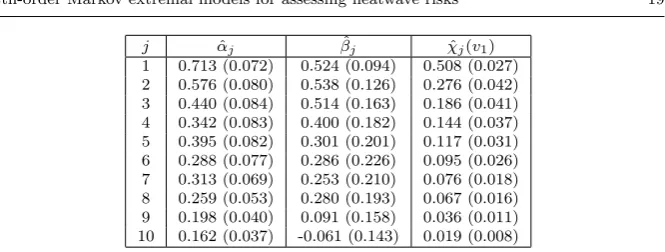
1 0.713 (0.072) 0.524 (0.094) 0.508 (0.027) 2 0.576 (0.080) 0.538 (0.126) 0.276 (0.042) 3 0.440 (0.084) 0.514 (0.163) 0.186 (0.041) 4 0.342 (0.083) 0.400 (0.182) 0.144 (0.037) 5 0.395 (0.082) 0.301 (0.201) 0.117 (0.031) 6 0.288 (0.077) 0.286 (0.226) 0.095 (0.026) 7 0.313 (0.069) 0.253 (0.210) 0.076 (0.018) 8 0.259 (0.053) 0.280 (0.193) 0.067 (0.016) 9 0.198 (0.040) 0.091 (0.158) 0.036 (0.011) 10 0.162 (0.037) -0.061 (0.143) 0.019 (0.008)

Table 1 Estimates for the extremal dependence parameters (αj,βj) and estimated extremal

dependence measure ˆχj(v1) for a set of different lag valuesj = 1, . . . ,10 at the one year return levelv1. The estimates ofχj(v) are obtained from the pairwise model forXt+j|Xt.

Standard errors are given in parentheses.

return level isv1= 35oC.

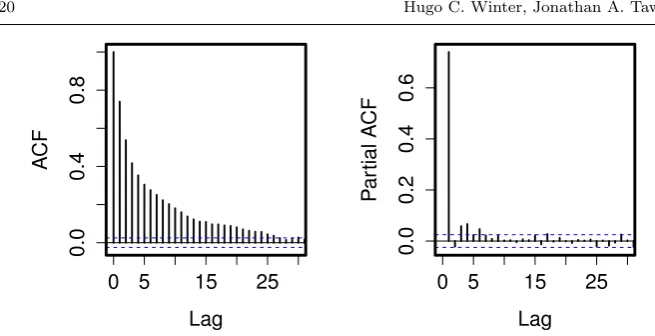
Before we examine the precise form of the extremal Markov process we in-vestigate how the extremal dependence decays with lag. Figure 1 (left) shows that the auto-correlation function for the Orleans daily maximum temperature data decays monotonically in a near exponential form. However, this estimate is dominated by the data in the body of the series and so may not reflect the extremal dependence.

To assess if this feature is observed for the extreme events we examine the extremal dependence parameters (α1:10,β1:10). Estimation uses a threshold corresponding to the 90% marginal quantile, with this level being selected based on the diagnostics proposed by Heffernan and Tawn (2004). Estimates (and standard errors in parentheses) of these parameters are given in Table 1. These estimates are obtained without making any extremal Markov process assumptions. The estimated values ˆα1:10are all statistically significantly differ-ent from one and zero, indicating the positive dependence form of asymptotic independence at lags 1−10. Furthermore, there is a general pattern of the val-ues decreasing with lag, though it is not entirely monotone. The ˆβ_1:10 exhibit a similar pattern. As ( ˆα1:10,βˆ1:10) are often correlated it is helpful to also consider a cluster functional estimate as the extremal dependence parameters combine to produce these. Here we examine the extremal dependence measure

χj(v1);j = 1, . . . ,10 estimated using the unconstrained parametric estimate, where ˆχj(v) is as described in Section 6. Table 1 shows that ˆχj(v1) decreases monotonically with increasing lag, so the pattern of dependence decay is sim-ilar for both typical and extreme values.

0 5 15 25

0.0

0.4

0.8

Lag

A

CF

0 5 15 25

0.0

0.2

0.4

0.6

Lag

P

ar

tial A

CF

Fig. 1 Auto-correlation function (left) and partial auto-correlation function (right) for Or-leans daily maximum temperature data. Dashed intervals represent a 95% tolerance inter-vals.

motivate their choice of a first-order Markov model. However, there are some values of the PACF that lie outside the 95% tolerance intervals up to lag 6. These values suggest that a first-order Markov model might omit some impor-tant higher-order structure and, as discussed in Section 6, this diagnostic may miss features of the extremal process.

We wish to examine whether there is statistically significant evidence for higher-order dependence than first-order for the process when in an extreme state, defined here to be when the process exceeds the 90% marginal quantile. A hypothesis test is constructed to test whether aτth-order dependence struc-ture provides a significantly better fit than a first-order approach. However, if the null hypothesis is rejected this only suggests that the true order of the extremal Markov process is greater than or equal to 2. The test is explained in Section 6. Under a first-order model the parameters (α2:10,β2:10) are con-strained to satisfy either condition (21) or (22), whereas for the τth-order model (α2:τ,β2:τ) are unconstrained. Tests are constructed forτ = 2, . . . ,10

and using Bonferroni bounds the significance level is set at 0.05/9. All tests for whichτ≥7 were found to be significant at the 5% significance level.

Section 5 set out that our main diagnostic for the selection of the order of the extremal Markov process is a comparison of estimates of χj(v) forj≥1. We have two reference estimates to compare our extremal Markov models to: non-parametric estimates ˜χj(v) whenv is low enough that empirical esti-mates ofχj(v) are reliable and the unconstrained parametric estimates ˆχj(v) for largerv. In each case we compare these estimates withτth-order extremal Markov model estimates ˆχ(_jτ)(v).

2 4 6 8 10 12 14

0.0

0.1

0.2

0.3

0.4

0.5

j χj

(

v

)

2 4 6 8 10 12 14

0.0

0.1

0.2

0.3

0.4

0.5

j χj

(

v

)

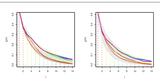
Fig. 2 Estimates of the threshold dependent extremal measureχj(v) using empirical

ap-proach (black) and different order extremal Markov chains (rainbow) withvset at 90% (left) and 95% (right) quantiles respectively. Grey shaded region corresponds to 95% confidence interval for empirical obtained via a block bootstrap approach.

that ˆχ(_jk)(v) is close to ˜χj(v) for all j for low v and to ˆχj(v) for highv.

Fur-thermore as

ˆ

χ_j(τ2)(v) = ˆχ_j(τ1)(v) for allj≤τ1< τ2,

our ability to distinguish between models of ordersτ1< τ2is only through the values of ˆχ(τ2)

j (v) and ˆχ

(τ1)

j (v) forj > τ1. Consequently in the plots of ˆχ

(τ)

j (v)

againstj in Figure 2 we select a different colour whenj > τ.

Figure 2 plots these diagnostics forvcorresponding to the marginal 90% and 95% quantiles (denoted v0.9 and v0.95). With v0.9 it appears that the third-order scheme comes closest to the pattern observed in the empirical estimates. First- and second-order schemes seem to underestimate the strength of the dependence whereas higher-order estimates seem to lead to an overestima-tion, reflecting their greater variation. Similar patterns are found for v0.95,

although the higher-order schemes seem to be contained within the empirical confidence bands for higher values ofj due to the increased uncertainty in the empirical estimate. Figure 3 shows the diagnostic forv =v1, which suggests that lower-order schemes are picking up the general behaviour better, being contained with the confidence intervals at all values ofj. However, the higher-order schemes do seem to pick up some higher-higher-order structure that is present in the original data set that is missed by a lower-order scheme. Taking all the diagnostics into account, we conclude that the third-order scheme seems to provide the most reliable estimates ofχj(v) at all levels.

prob-2 4 6 8 10 12 14

0.0

0.1

0.2

0.3

0.4

0.5

j χj

(

v1

)

Fig. 3 Estimates of the threshold dependent extremal measureχj(v1) using unconstrained

parametric estimates (black) and different order extremal Markov chains (rainbow). Grey shaded region corresponds to 95% confidence interval for unconstrained parametric approach obtained via a block bootstrap approach.

2 4 6 8 10 12 14

0.30

0.35

0.40

0.45

0.50

0.55

τ

θ

(

v1

)

2 4 6 8 10 12 14

0.40

0.45

0.50

0.55

0.60

τ

Π

(2,v

1

)

2 4 6 8 10 12 14

0.02

0.04

0.06

0.08

0.10

0.12

τ

Π

(6,v

1

)

2 4 6 8 10 12 14

0.000

0.005

0.010

0.015

τ

Π

(11,v

1

)

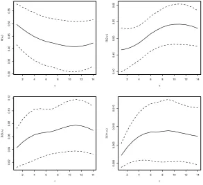
abilities of short and long events are of particular interest as these correspond the observed durations of the 2003 European heatwave at Orleans. We wish to assess the sensitivity of these cluster functional estimates to the choice of the order of the extremal process.

Figure 4 shows estimates of these cluster functionals for orders ofτ = 1. . . ,14 for the extremal Markov model. As explained in Section 6, we aim to iden-tify the lowest order for which these cluster functionals remain constant at all higher orders, other than for sampling variability. The uncertainty bounds used in this figure are obtained via the block bootstrap. As the accurate evalu-ation of cluster functional is computevalu-ationally intensive it is not feasible to run many bootstrap replications. Instead we run a reduced number of replications to approximate the standard error for the cluster functional sampling distri-bution and then construct symmetric confidence intervals around the point estimate using this standard error.

The estimates of the average duration of a heatwave and the probabilities of short, median and long clusters all increase when a higher-order extremal Markov chain is used. Typically the estimates increase rapidly until τ = 3, continue to increase until τ = 7 and then stabilise. However, this pattern is somewhat masked by the confidence intervals which broadly cover all esti-mates at all orders, so there is limited information about choice of the order. Of course we could have used a lower value of the critical level thanv1which would have been better for diagnostic purposes, but would not have shown the sensitivity issues of the features most relevant in practice. But even at level

v1 we find that for probabilitiesΠ(2, v1) our diagnostic suggests that we need

τ≥3.

8 Discussion and conclusion

This paper provides a new framework for incorporating higher-order Markov models for temporal dependence when modelling extreme events covering pro-cesses which can be either asymptotically dependent or asymptotically inde-pendent. For this purpose we have developed a kth-order extremal Markov model framework for incorporating higher-order information using the condi-tional extremes approach of Heffernan and Tawn (2004). Such an approach is motivated by an application to heatwave events, since all the existing time se-ries extremes models, which have been developed under assumptions of either a first-order Markov model or that the variables are asymptotically dependent, do not adequately capture the properties we observe for heatwaves.

Our results show that using standard time series diagnostics to identify the or-der of an extremal Markov process can lead to errors when interest is restricted to the extremes of the process. This necessitated the development of a range of new diagnostics for choosing the ‘best’ order scheme to use for extreme events. Specifically, in our example the use of standard time-series diagnostics ignored structure in the extremes which leads to the underestimation in the probabil-ity of longer and potentially devastating heatwave events. One area for further work is to formalise and unify our range of heuristic diagnostic methods for estimating the order of the extremal Markov process. To help achieve this a systematic study of the performance of these methods in a simulation study is needed. This study should cover both asymptotically independent and asymp-totically dependencekth-order Markov processes, each with varying strengths of dependence.

As in Winter and Tawn (2016), daily maximum temperatures have been anal-ysed instead of looking at the joint distribution of daily maximum and mini-mum temperatures. An extremal Markov model would still be appropriate in such a situation but a different order scheme might be required and stationar-ity be imposed separately on the maximum and minimum temperature series. The effect of climate change and other large scale climatic phenomena have not been incorporated into this paper. Winter et al (2016) illustrate how the tail chain simulation approach with first-order dependence structure can be altered to take into account the effect of covariates. A similar extension could be applied to the methodology outlined here.

References

Bortot P, Tawn JA (1998) Models for the extremes of Markov chains. Biometrika 85(4):851– 867

Brockwell PJ, Davis RA (2006) Introduction to Time Series and Forecasting. Springer Chatfield C (2003) The Analysis Of Time Series: An Introduction. CRC Press

Coles SG (2001) An Introduction to Statistical Modeling of Extreme Values. Springer Verlag Coles SG, Tawn JA (1991) Modelling Extreme Multivariate Events. Journal of the Royal

Statistical Society: Series B 53(2):377–392

Davison AC, Smith RL (1990) Models for exceedances over high thresholds (with discussion). Journal of the Royal Statistical Society: Series B 52(3):393–442

Davison AC, Padoan SA, Ribatet M (2012) Statistical modeling of spatial extremes. Statis-tical Science 27(2):161–186

Drees H, Segers J, Warchol M (2015) Statistics for tail processes of Markov chains. Extremes 18:369–402

Dunn OJ (1961) Multiple comparisons among means. Journal of the American Statistical Association 56(293):52–64

Dupuis DJ (2012) Modeling waves of extreme temperature: the changing tails of four cities. Journal of the American Statistical Association 107(497):24–39

Fawcett L, Walshaw D (2006) Markov chain models for extreme wind speeds. Environmetrics 17(8):795–809

Ferro CAT, Segers J (2003) Inference for clusters of extreme values. Journal of the Royal Statistical Society: Series B 65(2):545–556

Genest C, Ghoudi K, Rivest LP (1995) A semiparametric estimation procedure of depen-dence parameters in multivariate families of distributions. Biometrika 82(3):543–552 de Haan L, Ferreira A (2006) Extreme Value Theory: An Introduction. Springer, New York Heffernan JE (2000) A directory of coefficients of tail dependence. Extremes 3:279–290 Heffernan JE, Resnick SI (2007) Limit laws for random vectors with an extreme component.

The Annals of Applied Probability 17(2):537–571

Heffernan JE, Tawn JA (2004) A conditional approach for multivariate extreme values (with discussion). Journal of the Royal Statistical Society: Series B 66(3):497–546

Hitz A, Evans R (2015) One-component regular variation and graphical modeling of ex-tremes. ArXiv e-prints 1506.03402

Joe H (1997) Multivariate Models and Dependence Concepts. Chapman and Hall/CRC Keef C, Papastathopoulos I, Tawn JA (2013) Estimation of the conditional distribution of

a multivariate variable given that one of its components is large: Additional constraints for the Heffernan and Tawn model. Journal of Multivariate Analysis 115:396–404 Kulik R, Soulier P (2015) Heavy tailed time series with extremal independence. Extremes

18:1–27

Ledford AW, Tawn JA (1997) Modelling dependence within joint tail regions. Journal of the Royal Statistical Society: Series B 59(2):475–499

Ledford AW, Tawn JA (2003) Diagnostics for dependence within time series extremes. Jour-nal of the Royal Statistical Society: Series B 65(2):521–543

Liang KL, Self SG (1996) On the asymptotic behaviour of the pseudolikelihood ratio test statistic. Journal of the Royal Statistical Society: Series B 58(4):785–796

Lugrin T, Davison A, Tawn JA (2016) Bayesian uncertainty management in temporal de-pendence of extremes. Extremes 19:491–515

Papastathopoulos I, Tawn JA (2013) Graphical structures in extreme multivariate events. In: Proceedings of 25th Panhellenic Statistics Conference, pp 315–323

Papastathopoulos I, Strokorb K, Tawn JA, Butler A (2017) Extreme events of Markov chains. Advances in Applied Probability 49

Pickands J (1971) The two–dimensional Poisson process and extremal processes. Journal of Applied Probability 8:745–756

Reich BJ, Shaby BA, Cooley D (2014) A hierarchical model for serially-dependent extremes: A study of heat waves in the western US. Journal of Agricultural, Biological, and Envi-ronmental Statistics 19:119–135

Ribatet M, Ouarda TBMJ, Sauquet E, Gresillon JM (2009) Modeling all exceedances above a threshold using an extremal dependence structure: Inferences on several flood charac-teristics. Water Resources Research 45:W03,407

Rootz´en H (1988) Maxima and exceedances of stationary Markov chains. Advances in Ap-plied Probability 20:371–390

Smith RL (1992) The extremal index for a Markov chain. Journal of Applied Probability 29(1):37–45

Smith RL, Weissman I (1994) Estimating the extremal index. Journal of the Royal Statistical Society Series B 56(3):515–528

Smith RL, Tawn JA, Coles SG (1997) Markov chain models for threshold exceedances. Biometrika 84(2):249–268

Wadsworth JL, Tawn JA (2013) A new representation for multivariate tail probabilities. Bernoulli 19(5B):2689–2714

Winter HC, Tawn JA (2016) Modelling heatwaves in central France: a case study in extremal dependence. Journal of the Royal Statistical Society: Series C 65(3):345–365

Winter HC, Tawn JA, Brown SJ (2016) Detecting changing behaviour of heatwaves with climate change. Submitted