Some qualitative results for the quadratic function approximation

SOME QUALITATIVE RESULTS FOR THE

QUADRATIC FUNCTION APPROXIMATION

R.G. Brookes

and

A. W. Mcinnes

Abstract

By means of a detailed investigation of some particular examples, this paper attempts to

assess some qualitative properties of the quadratic function approximation. Particular attention

is paid to the size of the region over which this is a good approximation, and to comparisons of

the accuracy of the approximation with the more traditional Pade and Taylor approximations.

No. 46 November, 1988.

AMS Classification: 41A30, 41A21, 65D15

Key words and phrases: Hermite-Fade approximation, quadratic function approximation,

1. Introduction

In the previous report [2] the existence of local quadratic approximations to any analytic function

f (

x)

was established. The questions which we now attempt to answer, mainly by means of illustrative examples, are these:

(i) Can the approximation

y(

x ), unique in some neighbourhood of the origin, be extended to approximate

f(x)

over some larger region?

(ii) Does this method of approximation give significantly better results than more traditional methods (eg. Pade and Taylor approximations) and if so, for what types of functions?

2. Discussion

2 .

In what follows it will be assumed that

2.:::

ai( x

)y(

x )' = 0 and that i=O

(i) the ai(

x)

do not have a common factor (ii)

2.:::

ai( x

)y(

x

)i

cannot be factorised.

i.e. $polynomials

p(x),q(x),r(x),s(x),

such that

L:ai(x)y(x)i

=

(p(x)y(x)

+

q(x))(r(x)y(x)

+

s(x)).

It will be shown in later work that this is not a serious restriction.

It then follows (Hille [3] Theorem 12.2.1) that

y(

x)

(as defined in [2]) is analytic everywhere except possibly at the points x E C such that a_{2 (}

x)

= 0 (poles) and the points x E C such that

D(

x)

= 0 (branch points). It is clear that

y( x)

is single valued and analytic in any simply connected neighbourhood of the origin not including any of the above points. It will be assumed that

f (

x ), the function being approximated is single-valued, or at least, that we wish to approximate only one of its Riemann sheets. It is then clearly necessary to restrict the region of approximation,

R,

so that

y(

x)

is single valued on

R.

This consideration, with some additional information about

f (

x)

(for instance, the knowledge that /(

x)

is analytic on some region, or the approximate location of any singularities) turns out to give enough information to accurately approximate some functions over a wide area.

3. Examples

3.1 Example 1

3.1.1 The (2,2,2) approximation to log(l+x.)

Consider the

(2,2,2)

quadratic approximation to the principal branch of f(x) = log(l +x)

(with a cut taken along

{x

ER:

x

E (-oo,-1]}). Note that:

(i) (x2 - 6x -

6)f(x)

2 -

(9x

2

+

18x)f(x)

+

24x

2 =

O(x

8) so that (using results from [2])

the approximation is

( ) 9x

2_{+18x - x)-15x}2

+

_900x

+

₉₀₀

y x

=

2

(x

2 - 6x - 6)

with y(x)=f(x)+O(x7) .

(ii) D(x)

=

-15x4

+

900x3

+

900x2 so the roots of D(x) are x = 0 (twice)

x = -0.9839

x = 60.9839.

The roots of a2( x) are x = -0.8730, x = 6.8730. Consideration of the proof of Theorem 1 in [2] shows that each of these roots corresponds to a pole on only one of the sheets

. ( ) -a1 (x) - x)-15x2

+

900x

+

900

y x =

2a2(x)

( ) -a1 (x)

+

x)-15x

2

+

_900x

+

₉₀₀

Yl x

=

2a2 (x)

and a removable singularity on the other. A simple calculation or consideration of the later

graphs shows that

y(

x) has no poles and to ensure that

y(

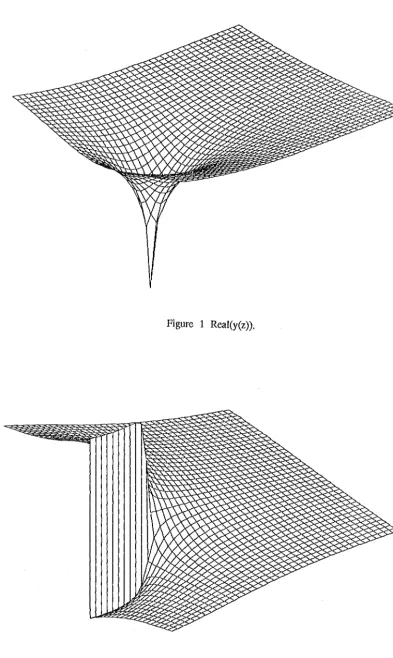
x) is single valued we simply need to · define its domain Ras C\ {x ER: x E (-oo,0.9839) or x E (60.9839,oo)}. Graphs of

y(z)

and the error function e( z) =

y(

z) - log(l

+

z) are now presented. These graphs are over the region

{x

+

iy EC:

lxl

~ 2,

lvl

~ 2} with mesh spacing of 0.1 using PC-Matlab. The point -2 - 2i corresponds to the lower left corner. It should be noted that some calculation error, particularly near z = -1 is inevitable but given that PC-Matlab uses double precision and that

it is understood that we are working with an open mesh, this effect is minimal.

Fig. I and Fig.2 are the real and imaginary parts respectively of the approximation. To

the naked eye these surfaces are virtually indistinguishable from those of log( 1

+

z)

(although lim log(l

+

t)

= oo -:/: y(-1)).

t-->-l

Figure 1 Real(y(z)).

Figure 2 lmag(y(z)).

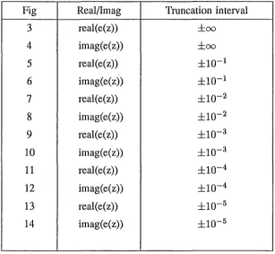
[image:4.617.108.502.91.750.2]

Graphs of the real and imaginary parts of the error function (clearly not exact at z = -1)

follow. These are shown truncated at successively smaller values so as to illustrate the error

behaviour throughout this region.

Fig Real/lmag Truncation interval

3 real(e(z)) ±oo

4 imag(e(z)) ±oo

5 real(e(z)) ±10-1

6 imag(e(z)) ±10-1

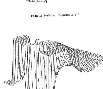
7 real(e(z)) ±10-2

8 imag(e(z)) ±10-2

9 real(e(z)) ±10-3

10 imag(e(z)) ±10-3

11 real(e(z)) ±10-4

12 imag(e(z)) ±10-4

13 real(e(z)) ±10-5

14 imag(e(z)) ±10-5

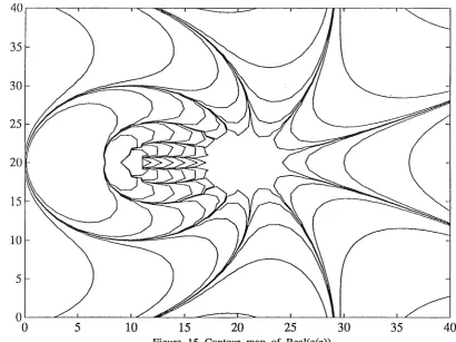
Fig. 15 and Fig. 16 are contour maps of the real and imaginary parts of

e(

z)

with contours drawn at {±10-3 _{±10-4 ±10-5 ±10-}6 _±10-7 _{±10-8 }}

'

'

'

'

'

' [image:5.597.155.463.188.471.2]

35 30 25 20 15 10 5

5 10 15 20 25 30 35 40

Figure 15 Contour map of Real(e(z)).

35 30 25 15 10 5

5 10 15 20 25 30 35 40

Figure 16 Contour map of Imag(e(z)).

[image:12.595.86.497.94.401.2] [image:12.595.79.502.213.733.2]

Comparison to a Pade approximation and to a Taylor polynomial.

In order to gauge whether the quadratic approximation is worthwhile it is useful to compare

its performance with those of the Pade and Taylor approximations which match

f (

x) to the same

order. Here we choose

p(x),

the (3, 3) Pade approximation and

t(x),

the Taylor polynomial of degree 6.

Note that

y (

x)

=

f (

x)

+

0 (

x

7)

p (

x)

=

f (

x)

+

0

(x

7)

t(x)=f(x)+O(x

7) .

3.1.2 The (3,3) Pade approximation to log(l+x).

The (3, 3) Pade approximation to log(l

+

x) is given by

llx3 - 60x2 - 60x

p ( x )

-- 3x3

+

36x2

+

_90x

+

₆₀

p(a:)

has poles at

x

= -8.87, -2.00, -1.13.

Graphs of the real and imaginary parts of

p(

z) follow. Because of the obvious difficulties, p(-2) has been set to zero.

Fig.17 and Fig.18 are the real and imaginary parts respectively of

p(

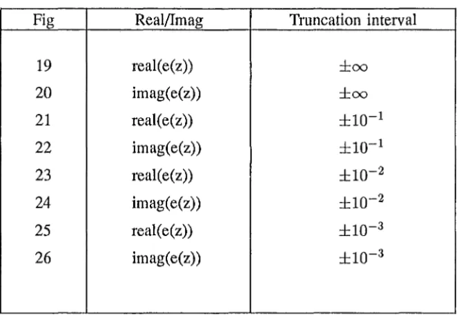
z ).

Graphs of the real and imaginary parts of the error function

e(z)

=

p(

z )-

log(l

+

z)

follow.

Fig Real/lmag Truncation interval

19

real(e(z)) ±oo

20

imag(e(z)) ±oo

21

real(e(z)) ±10-1

22

imag(e(z)) ±10-1

23

real(e(z)) ±10-2

24

imag(e(z)) ±10-2

25

real(e(z)) ±10-3

26

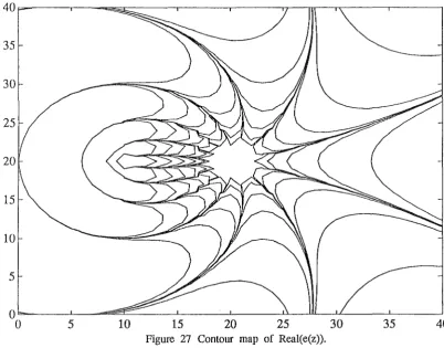
imag(e(z)) ±10-3

Figures 27 and 28 are contour maps of Real(

e( z))

and Imag(

e( z))

with contours drawn at {±10-3_,±10-4_,±10-5_,±10-6_,±10-7_{,±10-8 } as in the previous case.} [image:15.598.142.473.141.379.2]

Figure 23 Real(e(z)). Truncation ±10-2

Figure 24 Imag(e(z)). Truncation ±10-2

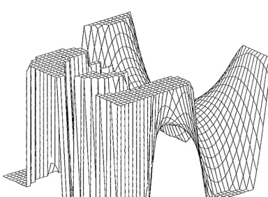
[image:18.615.100.487.126.364.2] [image:18.615.104.497.357.696.2]

Figure 25 Real(e(z)). Truncation ±10-3

Figure 26 Imag(e(z)). Truncation ± 10-3

[image:19.618.121.492.88.752.2] [image:19.618.118.503.448.731.2]

35 30 25 20 15 10 5 Qb-~~_t_~....,.;;;~:::_~~L-~~_l_~~~~--11L~L.L_~~_l_~~_J

0 5 10 15 20 25 30 35 40

Figure 27 Contour map of Real(e(z)).

35 30 25 20 15 10 5 o~~~~~~_,_~~~.__~_,__,,,,_~~_._~~~.__~_,_~_...~__._.

0 5 10 15 20 25 30 35 40

Figure 28 Contour map of Imag(e(z)).

[image:20.598.93.496.95.410.2]

Consideration of these pictures makes it clear that

y(

z)

(the quadratic function) is a considerably better approximation to

f(z)

than

p(z)

(the rational function) both around the origin and the branch point. Clearly the branch point structure of

y(z)

is very similar to that of

f(z).

3.1.3 The degree 6 Taylor polynomial approximation to log(l+x)

Finally graphs of

t(z),

the Taylor polynomial of degree 6 and the error function

e(z)

=

t(z)-

log(l

+

z)

are given.

t(z)

is clearly inferior to both

y(z)

and

p(z)

as an approximation.

Figures 29 and 30 are the real and imaginary parts of

t(

z ).

Figures 31 and 32 are the real and imaginary parts of e(

z)

truncated at

±

10-1.

Figures 33 and 34 are contour maps of Real(

e( z) ),

Imag(

e( z))

with contours drawn at {±10-3,±10-4,±10-5,±10-6,±10-7,±10-8} as in the previous cases.

35 30 25 20 15 10 5 o~~~~~~--'--~~~'---'-~~~~-'---'~~'--~~-'-~~~

0 5 10 15 20 25 30 35 40

Figure 33 Contour map of Real(e(z)).

35 30 25 20 15 10 5 0'--~~-'-~~-'--L-~~'--~~-'--'-~-'-~~---''---"~--'-~~--'

0 5 10 15 20 25 30 35 40

Figure 34 Contour map of Imag(e(z)).

3.2 Example 2

3.2.1 The (4,4,4) approximation to log(l+x). Note that :

(i)

(ii)

(6x4 - 360x3

+

180x2

+

1080x

+

540)

f

(x)2

+

(-75x4

+

1620x3

+

5310x2

+

3540x)

f (

x)

+

260x4 - 4080x3 - 4080x = 0 ( x14)

D

(x)

= -

615x8

+

229320x7 - 4136580x6

+

12612600x5

+

59667300x4

+

64033200x3

+

21344400x2 •

Let

d(

x) =

D(

x) / x2• Using the results of [2] the approximation is :

The roots of

d(

x)

are :

while the roots of

az ( x)

are :

( ) -

-ai(x)+x~

y x - _2a2 ( ) . x

x

=

354.0459

x = 10.8301

±

0.06444i x

=

.-0.9155

±

0.0005i

x = -0.9972

x

=

59.4440 x

=

2.2298

x

=

-0.6904

x = -0.9835.

To ensure that

y( x)

is single valued, cuts must be taken from the roots of d(

x ).

There are, of course, an infinite number of ways in which this may be done. It turns out that the

simplest method gives a very good approximation to log(l

+

x ). In the region presently under

consideration d( x) has 3 zeros. x = -0.9972 is close to the known branch point of

f (

x) at x = -1 and this point is treated as in the previous example by taking ( oo, -0.9072] as a cut. The other zeros are the conjugate pair x = -0.9155

±

0.0005i. A cut could be taken from each point towards oo but in view of the fact that

f (

x)

is analytic on C\ {

x

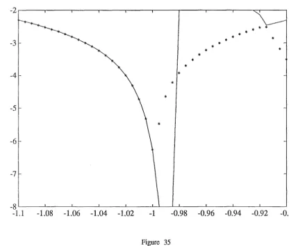
E R : :r E ( -oo, -1]}

this choice cannot be expected to give a good approximation. The other alternative is to take a cut between the two points. In fact the behaviour of the two possible values of

y(

x) on the real axis close to these points (Fig.35) suggests that the best choice is to take the cut { x

+

iy

E C : x = -0.9155,

Jyj ::::;

0.0005} . It is of interest to note that this choice of cuts ensures that none of the roots of

az( x)

are poles of

y( x ).

Fig. 35 shows the real parts of both possible continuations of

y(

x) along the real axis; one, Y+(x), denoted by a solid line, the other y_(x), by"*"· Y+(x), which is the analytic continuation of

y( x)

along the real axis, has a pole at

z

= -0.9835. The effect of taking the cut between the points z = -0.9155

±

0.0005i is to "jump" from Y+(x) to y_(x) at x

=

-0.9155. Fig.36 shows real(log(l

+

x )) (although real(log(O))

=

-oo) and Fig.37 shows simultaneously real(log(l

+

x)) and real(y( x)) our approximation.

-3 * -4 -5

*

-6 -7 * * * * * * * * * -8'--~--'-~~-'-~~-'-~~'--~-L--'---'--'-~~-'-~~'--~--'-~~-'

-1.1 -1.08 -1.06 -1.04 -1.02 -1 -0.98 -0.96 -0.94 -0.92 -0.9

Figure 35

[image:26.600.84.500.346.699.2]

-3 -4 -5 -6 -7 -8'--~-'-~~'--~-'-~~'--~-'-~~'--~-'--~~L..-~--L-~---J

-1.1 -1.08 -1.06 -1.04 -1.02 -1 -0.98 -0.96 -0.94 -0.92 -0.9

Figure 36

-3 -4 -5 -6 -7 -8'--~-'-~~'--~-'-~~'--~-'--'--_._'--~-'-~~'--~-'-~--J

-1.1 -1.08 -1.06 -1.04 -1.02 -1 -0.98 -0.96 -0.94 -0.92 -0.9

Figure 37

R ~

{x

+

iy

EC :

Jxl ::;;

2,

lvl ::;;

2} has now been defined. so that

y(z)

has a unique analytic continuation on R. It remains to calculate

y(z)

at points in R. Clearly it is not sufficient to just write

y

(z)

=

-ai(z)

+

x/d(Z)

2a2(z)

and the attempt to do so results in imag(y(

z))

behaving as in Fig.38.

Figure 38

It is necessary to follow a path inside R "analytically" from the origin to each point. The following algorithm is used for this "analytic" procedure.

[image:28.595.103.499.251.641.2]

Algorithm.

The process is given for the first quadrant only. The rest are similar. (Note that i2 _{= -1).}

sign= 1

dz(O, 0)

=

y'd(6)

argl = arg(dz(O,O))

For j = 0.1 step 0.1 to 2 do

dz(O,j)

= sign

/d[Jf)

arg2 = arg

(dz(O,j))

If largl - arg2I

>

2{ then

sign= - sign

dz(O,j)

=

-dz(O,j)

arg2 = arg

(dz(O,j))

end

argl = arg2

end.

Note that

dz(O,j)

now has the appropriate value of

/JN

for

z

= 0

+

ji. To cover the remainder of points we step outward in lines from the imaginary axis as follows :

For j = 0 step 0.1 to 2 do sign = 1

z = ji

argl

=

arg(

dz(

0,

j))

For'"= 0.1 step 0.1 to 2 do

z

=

k

+

ji

dz(k,j)

=sign

/JN

arg2 = arg

(dz( k, j))

If largl - arg2I

>

2; then

sign= - sign

dz(k,j)

=

-dz(k,j)

arg2 = arg

(dz(k,j))

end

argl = arg2

end

end

It now remains only to form the matrix

-ai(z)+zdz(k,j)

-k

.•

2a2 (

Z)

'

z -

+

J I

to get

y(

z)

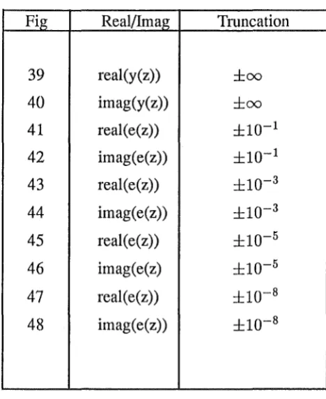
on all points of the mesh. Graphs of the real and imaginary parts of

y(

z)

and e(

z)

=

y( z) -

log( 1

+

z)

along with contour maps of real( e(

z))

and imag( e(

z))

are now presented.

Fig Real/Imag Truncation

39 real(y(z)) ±oo

40 imag(y(z)) ±oo

41 real(e(z)) ±io-1

42 imag(e(z)) ±10-1

43 real(e(z)) ±10-3

44 imag(e(z)) ±10-3

45 real(e(z)) ±10-5

46 imag(e(z) ±10-5

47 real(e(z)) ±10-8

48 imag(e(z)) ±10-8

Figures 45 and 50 are contour maps of real( e(

z))

and imag( e(

z))

with contours drawn at

{±10-3 _{± 10-4, ... '±10-8} .}

[image:30.597.188.422.268.554.2]

Figure 45 Real(e(z)). Truncation ±10-5

Figure 46 Imag(e(z)). Truncation ±10-5

[image:34.628.97.500.128.725.2] [image:34.628.102.501.476.709.2]

Figure 47 Real(e(z)). Truncation ±10-8

[image:35.621.112.491.82.754.2]

30

25

20

15

10

5 10 15 20 25 30 35 40

Figure 49 Contour map of Real(e(z)).

35

30

25

15

10

5

5 10 15 20 25 30 35 40

Figure 50 Contour map of Imag(e(z)).

3.2.2 A comparison with the (6,6) Pade approximation to log(l+x).

Note that

49x6

+

1218x 5

+

7980x4

+

20720x3

+

23100x2

+

9240x p ( x) = 10x6

+

420x5

+

420Qx4

+

16800x3

+

_31500x2

+

_27720x

+

₉₂₄₀

and that

y(x)

=

f

(x)

+

0

(x

13)

p(x)

=

f

(x)

+

0

(x

13) •

Figures 51 and 52 are graphs ofreal(p( z)) and imag(p(

z))

while figures 53 and 54 are contour maps of real( e(z)) and imag(

e(z ))

with contours drawn at {±10-3, ±10-4, ... , ±10-8 } •

Clearly

p(x)

is inferior to

y(x)

as an approximation and examination of the Taylor polynomial of degree 12 shows that it is still less accurate.

35 30 25 15 10 5

5 10 15 20 25 30 35 40

Figure 53 Contour map of Real(c(z)).

35 30 20 15 10 5

5 10 15 20 25 30 35 40

Figure 54 Contour map of Imag(e(z)).

[image:39.595.95.499.97.778.2]

3.3 Example 3

3.3.1 The (2,2,2) approximation to e-x •

Note that

so that

(x2 + 9x + 24) f (x)2 - (8x 2 +48) f(x) + x2 -9x + 24

=

0 (x8)

y(x)=

8x2+48-xV60x2+900

=J(x)+O(x1).

2(x2+9x+24)

Figures 55 and 56 are graphs of real(y(z)) and imag(y(z)) while figures 57 and 58 are

contour maps ofreal(

e(z ))

and imag( e(z )) with contours drawn at {±10-3, ±10-'1, •.• , ±10-8}

35 30 25 20 15 10 5

5 10 15 20 25 30 35 40

Figure 57 Contour map of Real(e(z)).

35 30 25 15 10 5

5 10 15 20 25 30 35 40

Figure 58 Contour map of Imag(e(z)).

[image:42.598.88.496.95.753.2]

3.3.2 A comparison with the Taylor polynomial of degree 6 .

The Taylor polynomial approximation to e-x, of degree 6 is

x2 x6 7

t(x)=l-x+

21 - ...

+6T=f(x)+O(x).

Figures 59 and 60 are the usual contour maps of real(

e( z))

and imag(

e( z)) .

Certainly

t(

x)

is inferior toy(

x)

but the difference is markedly less dramatic than with log(l

+x) .

This is to be expected since e-x is a smoother function, with a faster converging power series than log(l

+x) .

5 10 15 20 25 30 35 40

Figure 59 Contour map of Real(e(z)).

35

30

25

15

10

5

5 10 15 20 25 30 35 40

Figure 60 Contour map of Imag(e(z)).

[image:44.595.75.508.88.763.2] [image:44.595.90.499.95.407.2]

3.4 Example 4

3.4.1 The (5,5,5) approximation to e-x •

Note that

so that

(x5

+

45x4

+

885x3

+

9450x2

+

54495x

+

135135)

f

(x )2

+ (

64x5

+

7680x3

+

161280x)

f

(x)

+

(x

5

- 45x4

+

885x3 - 9450x2

+

54495x - 135135) = 0 (x17)

t x _ -64x5 - 7680x3 - 161280x

+

./D(X)

_

x

0 x17 1J ( ) - 2 (x5

+

_45x4

+

_885x3

+

_9450x2

+

_54495x

+

_{135135) -}

f ( )

+ (. ) '

where

D ( x) = 4092x10

+

984060x8

+

79459380x6

+

2497294800x4

+

24348624300x2

+

73045872900

Figures 61 and 62 are contour maps of real(

e(

z)) and imag(

e(

z)) this time with contours drawn at {±10-6,±10-7 , •.. ,±10-11 }.

35 30 25 20 15 10 5

5 10 15 20 25 30 35 40

Figure 61 Contour map of Real(e(z)).

35 30 25 20 15 10 5

5 10 15 20 25 30 35 40

Figure 62 Contour map of Imag(e(z)).

[image:46.603.94.502.88.782.2] [image:46.603.98.500.91.412.2]

3.4.2 A comparison with the Taylor polynomial of degree 16 .

Note that

t(x)

=

J(x)

+

O(x

11).

Figures 63 and 64 are contour maps of real(

e( z))

and imag(

e( z))

with contours drawn at

{±10-6' ... '±10-11} .

35

30

20

10

5

5 10 15 20 25 30 35 40

Figure 63 Contour map of Real(e(z)).

35 30 25 20 15 10 5

5 10 15 20 25 30 35 40

Figure 64 Contour map of Imag(e(z)).

[image:48.605.100.500.96.403.2]

4. Conclusion

This paper has attempted to assess some qualitative prope1ties of the quadratic approximation by means of detailed investigation of some particular examples. Particular attention was paid to the size of the region over which this was a good approximation and to comparisons of the accuracy of the quadratic approximation with the more traditional Pade and Taylor approximations. An algorithm for obtaining a smooth, analytic approximation over the wider region was given.

It is clear from these examples that when using the quadratic approximation, care must be taken in defining the region of the approximation, and particularly in the placement of cuts from the branch points. However if this is done in a sensible manner, the approximations in these examples appear to be significantly better than the usual approximations, particularly for a function with some branch point structure. It is also of interest to note that the approximation is able to accurately represent this branch point structure. It is apparent from the contour maps of the error function, that the quadratic approximation to the log function is at least two significant figures better than the corresponding Pade approximation.

The function exp(

-x)

was used as an example of a smooth function. The quadratic approximation to this function is also an improvement over the traditional approximations. However, the roughly one significant figure improvement in the error over the corresponding Taylor polynomial approximation does not appear to justify the additional computational cost for functions of this type. It is interesting to compare these results with the specific numerical results obtained by Borwein [l].

References

1. P.B. Borwein (1986) : Quadratic Hermite-Pade Approximation to the Exponential Function. Constr. Approx., 2 : 291-302.

2. R.G. Brookes, A.W. Mclnnes (1988) : The existence and local behaviour of the quadratic function approximation. Math Research Report 45, University of Canterbury.

3. E. Hille (1962) : Analytic Function Theory, vol II. Boston : Ginn and Company.