Integrated Traffic Control with Variable Speed Limits and Coordinated Ramp Metering based on Traffic Stability

Integrated Traffic Control with Variable Speed Limits and

Coordinated Ramp Metering based on Traffic Stability

Oskar A.L. Eikenbroek

Integrated Traffic Control with Variable Speed Limits and

Coordinated Ramp Metering based on Traffic Stability

by

Oskar A.L. Eikenbroek

s1003518

July 29, 2013

University of Twente

California PATH, University of California, Berkeley

April to July, 2013

Summary

For the last decades, congestion on highways has been a serious issue. Congestion causes more air pollution, accidents and delays, resulting in late arrival for employment or meetings. One of the main goals of the field of transportation engineering is to reduce or prevent delays and accidents caused by congestion, although, the last years it has been becoming more apparent that congestion cannot be completely solved. The main reason is simple; the highways are carrying too much vehicle miles, more than for it was designed

At first sight, an easy way to resolve congestion is the construction of new roads. By constructing new roads the capacity of the highway system will be higher and the number of traffic jams will be reduced, but is an expensive solution. Innovative solutions such as ramp metering and vari-able speed limits can be used to reduce congestion on a highway. In order to resolve or prevent congestion essential is the predictability of congestion.

Congestion is a result of a combination of three ingredients; a high traffic volume, a local per-turbation and a spatial inhomogenity. Studies by Lee et al. (2000) and Treiber et al. (2000) have shown that the relation between these three ingredients can be predicted by traffic stability. The influence of a local perturbation (e.g. a lane change) on the flow can eventually cause congestion if the traffic flow is unstable. This validates that it is essential to measure the stability of traffic flow.

Two discussed stability indicators are able to determine the stability of traffic in free flow. A stochastic approach is able to determine whether traffic has entered the metastability regime (only large perturbations lead to congestion) and a reliability indicator, based on the variance in flow, is able to determine the stability.

To make sure congestion will not arise, traffic can be controlled. Two control strategies, ramp metering and variable speed limits, are discussed. Ramp metering strategies control the amount of vehicles entering the mainline. Literature has shown that local and coordinated ramp metering strategies are able to improve the efficiency of a highway. Variable speed limits can be used in order to homogenize traffic or to prevent traffic breakdown by limiting the inflow of a highway segment. The homogenization approach is, based on the definition of traffic stability, causing a lower capacity. The more complex approach, preventing breakdown, is able to reduce travel time as simulation studies have shown an improvement of travel time up to 50 % (Lu et al., 2011; Su et al., 2011).

As it was shown that ramp metering strategies and variable speed limits are able to reduce travel time and stability indicators are able to predict congestion, these two are combined for new control strategies. Based on a local ramp metering strategy, a correction factor is proposed based on traffic stability. If traffic flow is unstable fewer vehicles should be allowed to enter the highway, if traffic stable the correction factor is high. Further research is needed to determine the performance and the influence of infrastructure layout and flow characteristics on the correction factor.

An integrated control strategy, where the variable speed limit is determined before the ramp meter rate, is proposed based on the preventing breakdown approach. As the detector measurements show that traffic is getting unstable, the control is switched on. Here, the speed limit on a highway segment is based on the difference between the desired and the measured occupancy. After the variable speed limits are set, a model predictive control scheme is used to find the optimal ramp meter rate. Every detector interval (30 seconds) the control scheme minimizes the total travel time and maximizes the total traveled distance. These calculations are used for implementation.

The proposed strategies are implemented in the simulation environment in order to test their per-formance. The network, modeled in the microsimulation software Aimsun, is a part of the I-880 NB in California, USA. Implemented in the simulation software is the section from post mile 9

vi

(Dixon Landing Road, Milpitas) to post mile 18.66 (Central Ave, Fremont). Five different strate-gies are compared; the uncontrolled case, the local ramp metering strategy ALINEA, the proposed variable speed limit strategy, the proposed coordinated ramp metering strategy and the proposed integrated strategy. Results show that the integrated strategy is best performing, improving the to-tal time spent with 6 %. Other control strategies show less improvement and the ALINEA strategy shows even less performance. The results are in line with literature but show less performance, expectedi s that the short on-ramps are highly influencing the performance. Concluded is that the control strategy is able to resolve the congestion earlier.

Acknowledgements

This thesis marks the end of my Bachelor programme Civil Engineering at the University of Twente and is the result of an 11-week during research at the California Partners for Advanced Transportation TecHnology (PATH), part of the Institute for Transportation Studies at the Univer-sity of California, Berkeley.

I would like to express my gratitude to my daily supervisors, Dr. Steven Shladover and Dr. Xiao-Yun Lu. Steven, thank you for giving me the opportunity to come to California and your feedback. Xiao-Yun, thank you for your help, your advice and the useful critiques. Special thanks to Dr. Danjue Chen for her help with Aimsun, which was a hard struggle. Thanks to all colleagues at PATH for answering my questions, I have had a wonderful time.

Special thanks go to Dr. Tom Thomas, supervisor at the University of Twente. Thank you for the interesting discussions about the topic of my research, although, finally, my research topic turned out different. I am grateful to you for the feedback to my preliminary and interim report.

I am grateful to the Dutch Ministry of Transport, Public Works, and Water Management - Rijk-swaterstaat - Centre for Transport and Navigation and Dr. Andreas Hegyi from the TU Delft for providing the SPECIALIST traffic data. Thanks to Enrique Vallejo for his help with my visa and thanks to my roommates in Berkeley for a great time.

Finally, I wish to thank my parents, friends and my girlfriend for their support.

Contents

Summary v

Acknowledgements vii

Contents ix

1 Introduction 1

2 Research Objective and Approach 3

2.1 Research Objective . . . 3

2.2 Research Questions . . . 3

2.3 Research Methodology . . . 4

2.4 Research Relevance . . . 4

2.4.1 Theoretical Relevance . . . 4

2.4.2 Practical Relevance . . . 4

2.5 Institute: PATH . . . 5

2.6 Overview . . . 5

3 Background 7 3.1 Congestion Causes . . . 7

3.2 Microscopic Traffic Characteristics . . . 7

3.3 Macroscopic Traffic Characteristics . . . 8

3.4 Traffic Stability . . . 10

3.4.1 Classification of traffic stability . . . 10

3.4.2 Indicating Stability . . . 10

3.5 Conclusion . . . 11

4 Traffic Control 13 4.1 Traffic Control . . . 13

4.1.1 Demand for Traffic Control . . . 13

4.1.2 Traffic Control Objectives . . . 13

4.1.3 Principles of Traffic Control . . . 14

4.2 Ramp Metering . . . 14

4.3 Variable Speed Limits . . . 15

4.4 Conclusion . . . 16

5 Control Strategy based on Traffic Stability 17 5.1 Local Ramp Metering Strategy . . . 17

5.2 Integrated control . . . 18

5.2.1 Speed Limit Design . . . 19

5.2.2 Optimal Ramp Meter Rate . . . 21

5.2.3 Discussion . . . 25

5.3 Conclusion . . . 25

6 Case Study 27 6.1 Simulation . . . 27

6.1.1 Introduction . . . 27

6.1.2 Selection . . . 27

6.1.3 Implementation . . . 28

6.2 Traffic Scenario . . . 29

CONTENTS x

6.3 Set-up . . . 29

6.3.1 Number of simulation runs . . . 30

6.3.2 Parameter Settings . . . 30

6.4 Results . . . 31

6.5 Discussion . . . 32

6.6 Conclusion . . . 34

7 Conclusions 35 7.1 Conclusions . . . 35

7.2 Further Research . . . 37

7.3 Research contributions . . . 38

7.4 Discussion . . . 38

7.5 Conclusion . . . 38

Bibliography 39 A Stability Indicators 43 A.1 Classical indicator . . . 43

A.2 Reliability indicator . . . 46

A.3 Conclusion . . . 46

B Traffic Control 49 B.1 Ramp Metering . . . 49

B.1.1 Ramp Metering Strategies . . . 49

B.2 Speed Limits . . . 52

B.3 Conclusion . . . 52

C Model Development 53 C.1 Aimsun . . . 53

C.2 Model Development . . . 53

C.2.1 Study Purpose, Scope and Approach . . . 53

C.2.2 Data Collection and Preparation . . . 55

C.2.3 Base Model Development . . . 55

C.2.4 Error Checking . . . 55

C.2.5 Microsimulation Model Calibration . . . 55

C.2.6 Alternative Analysis . . . 57

C.2.7 Final Report . . . 58

C.3 Discussion . . . 58

D Calibration Results 59

1

Introduction

For the last decades, congestion on highways has been a serious issue. Congestion causes more air pollution, accidents and delays, resulting in late arrival for employment or meetings. One of the main goals of the field of transportation engineering is to reduce or prevent delays and accidents caused by congestion. The last years, it has been becoming more apparent that congestion cannot be completely solved. The main reason is simple; the highways are carrying too much vehicle miles, more than for it was designed.

At first sight, an easy way to resolve congestion is the construction of new roads. By constructing new roads the capacity of the highway system will be higher and the number of traffic jams will be reduced. It has been becoming clear that it is impossible to construct extra roads to meet the demand of vehicle miles; new roads will cause a higher demand. Increasing the capacity of the existing road network, without the construction of new roads, requires innovative solutions. Traffic flow control, such as ramp metering, route guidance, driver information systems and variable speed limits, can be used to improve traffic flow, traffic safety and to reduce the environmental impact.

Basically, congested traffic is the result of a too high demand. If the demand for a highway section is exceeding the supply (bottleneck) a traffic jam arises. Empirical findings by Treiber & Kesting (2013) have shown that bottlenecks on highways is the result from a combination of three ingredients; high traffic volume, spatial inhomogenity and temporary perturbations of the traffic flow. These three ingredients come together in a bottleneck and causes a limited flow upstream of the bottleneck, approximately 5 to 20 % below its capacity (Lu et al., 2010b). So, the highway carries, during congestion, less vehicle miles than it was designed for.

Several methods have been proposed in the past to limit congestion and to improve the flow on highways. The last decade a lot of studies were done proposing ramp metering of an on-ramp and/or setting variable speed limits to homogenize or to limit the inflow of traffic. The most of the approaches are very complex but show an improvement of total travel time between 10 and 20 %. A simulation study of Lu et al. (2011) reported even a decrease of 50 % in travel time on the I-80 highway in California, USA.

Essential in proposing different traffic control strategies is the predictability of the network. If it is possible to predict where congestion arises and how long it takes before it disappears, it is more feasible to find a solution. Therefore, the most highways are supplied with detectors. These detectors measure several characteristics of a traffic flow and based on these characteristics it is possible to measure the congestion. More complex methods are required to predict the location and the ’amount’ of congestion.

Studies by Lee et al. (2000) and Treiber et al. (2000) have shown that the type of congestion can be predicted using the fundamental diagram. Lee et al. (2000) made an empirical study of a highway, and found a relationship between the on-ramp and upstream highway flow and the type of congestion that arises. Treiber et al. (2000) further identified these types of congestions and proposed a theory for several macroscopic and microscopic models in which it is possible, based on the flow and stability, to predict which kind of congestion will arise. These studies have shown that based on traffic stability one is able to predict congestion. However, this theory has not been used previously for improving traffic flow and lowering the travel time. This report proposes an integrated traffic control strategy to improve travel time based on traffic stability.

2

Research Objective and Approach

Congestion is an undesired phenomenon on the highway and can be limited by constructing new roads or using innovative solutions such as ramp metering and variable speed limits. If it is possible to predict the congestion on the highway, it is more feasible to prevent or resolve congestion. It was shown (Lee et al., 2000; Treiber et al., 2000) that using the stability of traffic one can predict congestion. Goal of this research is providing a traffic control strategy based on traffic stability.

2.1

Research Objective

Studies by Lee et al. (2000) and Treiber et al. (2000) have shown that stability of traffic gives a prediction about the arising of congestion. Central in this report is measuring the stability with existing measuring techniques, and based on these measurements developing a traffic control strat-egy. As a wide range of traffic control strategies are available, only two strategies (ramp metering and variable speed limits) are used which have proven their performance. The research objective is defined as follows:

Developing a variable speed limit and coordinated ramp metering strategy based on traffic stability.

As it is essential to measure the performance of the strategy, the control strategy will be tested on a part of the I-880 highway in California, USA in a simulation environment.

2.2

Research Questions

A central research question is formulated, derived from the research objective:

How can congestion be limited using a variable speed limit and coordinated ramp metering strategy based on traffic stability?

In order to answer the central research question and to reach the research objective, the following sub research questions are formulated:

What is traffic stability and how can it be measured using existing measuring techniques?

How can traffic stability contribute limiting the congestion on highways?

How can variable speed limits and coordinated ramp metering improve traffic flow?

What is the microsimulation performance of the control strategy on the I-880 highway in California, USA?

How can the control strategy be best introduced in the real world given the simulation results?

2.3. RESEARCH METHODOLOGY 4

2.3

Research Methodology

This research consists out of two phases, a literature study and a simulation study. First of all, a literature study will be made. Literature gives insight into the concept of traffic flow theory and how the dynamics of congestion can be described. Literature will also gain insight into the current measurement techniques and whether these techniques are able to explain the arising of congestion. The theory of traffic stability will be investigated and stability indicators will be tested in order to measure the stability of traffic.

In order to control traffic, a lot of variable speed limits and controlled ramp metering have been developed the last years. Strategies for ramp metering, variable speed limits, as well as the com-bination of these strategies, will be discussed including their contributions to limit congestion on highways. The strategies can be used for expansion or as starting point for a new approach. Based on the theory of traffic stability and traffic control strategies, a strategy will be proposed to limit or prevent congestion.

As the strategy is formulated, the second phase of the research is a microsimulation study. Simula-tion is a powerful technique to determine the performance of the strategy. The simulaSimula-tion software Aimsun will be used to model traffic of the I-880 Northbound on one particular day. Goal of the simulation study is measuring the performance of the combined variable speed limit setting and the coordinated ramp metering strategy and comparing the performance with the uncontrolled case. It is clear that one day is not sufficient to give a good approximation of the results in real world, but just limited time is available.

To determine the performance of the strategy, first, the I-880 Northbound highway needs to be modeled into the simulation software. It is essential that the model mirrors real world behavior, therefore, the model needs to be calibrated. After calibration, simulations will be made comparing the strategy and the uncontrolled case. The performance will be based on efficiency; the less time individuals spent on the highway and the better the performance.

Finally, the outcomes of the literature and simulation study will be used to give recommendations for application of the algorithm in real world and it will be used to give recommendations for future research.

2.4

Research Relevance

2.4.1 Theoretical Relevance

Investigating how existing measurement techniques are able to determine traffic stability, including their limitations, could be contributing to the existing publications about traffic stability (summa-rized in Pueboobpaphan & van Arem (2010)).

Lots of literature is available about setting variable speed limits and/or using controlled ramp metering. On the other hand, no literature (with exception: Elbers (2005)) is available improving travel time based on the stability of traffic flow. This research might give new insights into setting speed limits and/or with coordinated ramp metering.

2.4.2 Practical Relevance

5 2. RESEARCH OBJECTIVE AND APPROACH

2.5

Institute: PATH

The research is conducted in the United States of America at the California Partners for Ad-vanced Transportation tecHnology (PATH) in Richmond, CA. PATH was established in 1986 as the California Program on Advanced Technoloy for the Highway and is part of the Institute of Transportation Studies, University of California in Berkeley in collaboration with Caltrans. In 2011 PATH has merged with the California Center for Innovative Transportation. PATH’s mission is to develop solutions to the problems of California’s surface transportation systems through cut-ting edge research, divided into three program areas (Transportation Safety, Traffic Operation and Modal Applications). PATH has 45 full-time staff members and supports the research of nearly 50 faculty members and 90 graduate students.

2.6

Overview

The report is structured as follows:

Chapter 3 gives an introduction to traffic congestion. It describes how congestion can be modeled using three ingredients of the arising of congestion. The influence of the ingredients on congestion is described using traffic stability. In this chapter, the arising of congestion and the predictability of congestion using stability indicators are discussed.

Chapter 4, Traffic Control, focuses on improving the efficiency of the network. Based on traffic control objectives, control strategies using variable speed limits and ramp metering are compared and their performance in other studies are indicated.

The theory of traffic stability and traffic control is used, in Chapter 5, in order to provide a local ramp metering and an integrated control strategy.

The integrated control strategy is tested on the I-880 Northbound highway in California, in a simulation environment. The results are compared to other studies and several improvements are suggested.

3

Background

This chapter delivers a theoretical framework for modeling traffic flow, a discussion of congestion causes and, based on traffic stability and two methods to predict traffic congestion.

3.1

Congestion Causes

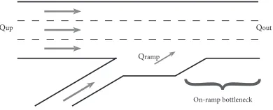
Empirical research (Schönhof & Helbing, 2004; Carlson et al., 2010) has shown that congestion (indicated by lower speeds and longer trip times (Bertini, 2006)) on the highway is the result of a combination of (i) high traffic volume, (ii) a spatial inhomogenity and (iii) a temporary pertur-bation. Considering an example of an on-ramp merging into a highway, a bottleneck can arise as the total traffic volume of the mainline and the on-ramp is high, the lane drops and an individual makes a lane changing maneuver (leaving the merging-lane). Clear is that congestion is caused by a stream of vehicles (macroscopic traffic characteristic), the infrastructure layout and an individual vehicle (microscopic traffic characteristic).

}

On-ramp bottleneck Qup

Qramp

Qout

ramp

Figure 3.1 Schematic indication of an on-ramp bottleneck. Three ingredients for congested traffic

are available; high traffic volume (Qup+Qramp), a spatial inhomogenity (merging lane drop) and

perturbations caused by the merging vehicles.

3.2

Microscopic Traffic Characteristics

In microscopic traffic theory each vehicle is considered individually. The microscopic approach is focusing on describing the detailed manner in which one vehicle follows another (Gartner et al., 2001), the longitudinal behavior of traffic, and on the lane changing behavior of traffic; the lateral driving behavior.

Considering vehicles are in the same lane of a road, longitudinal driving behavior describes the relationships between a follower and a leader. If the distance between the rear bumper of the predecessor and the front bumper of the following vehicle (gap) is too small, unsafe conditions can occur. In order to obtain a safe gap between vehicles, individuals can brake or change lanes (lateral driving behavior). To make sure the gap is large enough, one can change lanes to improve driving conditions, the so-called discretionary lane change (DLC). If the lane change is required due to e.g. a lane drop, one speaks of a mandatory lane change (MLC). As was indicated (Schönhof & Helbing, 2004) a MLC is caused by a spatial inhomogenity and is causing a temporary perturbation (two of the three congestion ingredients).

The process from considering a lane change to making the maneuver is modeled by Ahmed et al. (1996) and is described as a four step process:

1. Decision to consider a lane change; drivers who want to make a lane changing maneuver estimate the space they need and estimate the available space. Based on this comparison,

3.3. MACROSCOPIC TRAFFIC CHARACTERISTICS 8

they decide to make a maneuver or to postpone it. The required space is dependent on several characteristics of the driver, the vehicle and the road. An individual has to perceive all the characteristics, before coming to a decision. Gipps (1986) formulated six factors (physically possible, location of obstructions, presence of designated lanes, intended turning movement, speed and presence of heavy vehicles) for those considering changing lanes.

2. Choice of a target lane; an individual is considering the possible target lanes. In case of an on-ramp the target lane is clear, one wants to change lanes to the left (for right-hand traffic countries).

3. Acceptance of gaps in target lane; a lane change will only take place if the given gap, to the predecessor and the following vehicle in the target lane, is acceptable (in perception of the subject vehicle). These acceptable gaps should be higher than the minimum acceptable gaps (critical gap), and differ for the lead (target predecessor) and lag (target follower) vehicle. Most gap acceptance models describe the acceptance of a gap stochastically. The critical gap is, based on the MLC-models from Ahmed et al. (1996) and Lee (2006), changing over time and dependent on the volume of traffic on the mainline, the average speed in the mainline, and, majorly, depending on the remaining distance to the end of the merging lane (in case of an on-ramp).

4. Performing the lane change maneuver; if a vehicle wants to make a lane change, has chosen the target lane, and considered the gaps as acceptable, the maneuver is made. In the target lane the lag vehicle wants to remain, after the lane change, a safe gap to its new predecessor and therefore a lane change (local perturbation) can cause a new lane change or a braking vehicle.

The model of Ahmed et al. (1996) identifies that making a MLC is highly dependent on individual behavior. Individuals, approaching the end of the merging lane (due to busy mainline traffic), are getting impatient, accept small gaps which triggers a braking maneuver in the target lane. The follower of the braking vehicle also tries to keep a safe distance to its predecessor; therefore a new braking maneuver is triggered. One will only observe this behavior if the vehicles in the mainline are impeded by each other, in other words: if traffic volume is high.

3.3

Macroscopic Traffic Characteristics

The total volume of traffic is one of the ingredients of the cause of congestion. Here, traffic is considered as a fluid, instead of considering each vehicle separately. The macroscopic traffic theory describes traffic on a system level and consists out of the flow rate (or volume), density and mean speed. Flow rate (q) is defined as the number of vehicles passing a point in a given period of time, usually expressed as an hourly flow rate per lane. The flow is based on vehicle counts in a time period. Traffic density is the number of vehicles occupying on a length of road. It gives an indication how crowded a road section is. The density can be found by making an aerial photograph of a road segment and counting the number of vehicles in a single, one mile (or kilometer) long, lane. The density differs from 0, indicating no vehicle on the lane, to a maximum value, representing vehicles are bumper to bumper. As indicated, it is hard to measure the density of a road section. A widely used technique in the USA, loop detectors, is measuring the occupancy (o). Occupancy is the fraction of time that vehicles are over the detector, and is based on the detector interval, the length of the vehicle, length of the detector and the vehicles speed. Occupancy and density are constants of each others. The final macroscopic traffic flow characteristic is the mean (or harmonic) speed, expressed in miles (or kilometers) per hour. The mean speed differs from the velocity. The mean speedu is the total distance traveled by all the vehicles in the region, divided by the total time spent in the region. It equals the sum of the speed of all vehicles divided by the number of vehicles.

9 3. BACKGROUND

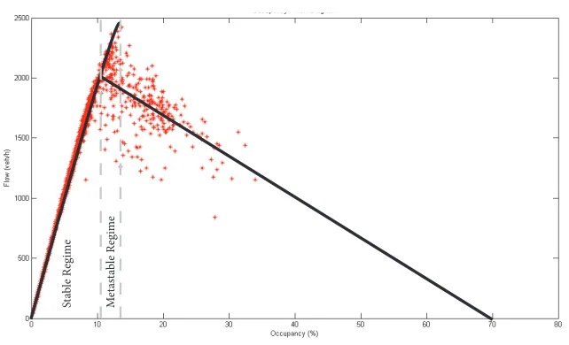
et al., 1935). This fundamental relation of traffic flow theory provides a bond between flow, density (or occupancy) and mean speed:q =ku. This relationship is visualized in a fundamental diagram (Figure 3.2), and plays a crucial role in traffic modeling. The fundamental diagram separates the traffic fluid from all other fluids and provides a static relation between the three macroscopic traf-fic characteristics. Empirical fundamental diagrams (Figure 3.3) show a more scattered pattern of flow, (in this case) occupancy and speed. This is because a theoretical diagram makes two as-sumptions; traffic is stationary (flow rates do not change over time and space) and homogeneous (all vehicles are equal) (Immers & Logghe, 2002). However, in traffic flow modeling the theo-retical fundamental diagrams are used, which can be validated by ’recognizing’ the theotheo-retical fundamental diagram in the empirical diagrams.

(a) Flow - speed (b) Density - Speed (c) Density - Flow

Figure 3.2 Three related fundamental diagrams, assuming that traffic is stationary and

homoge-neous (Immers & Logghe, 2002).

0 500 1000 1500 2000 2500 10 20 30 40 50 60 70 80 90 100

Flow − Speed Diagram

Flow (veh/h)

Speed (mph)

(a) Flow - speed

0 5 10 15 20 25 30 35 10 20 30 40 50 60 70 80 90 100

Occupancy − Speed Diagram

Occupancy (%)

Speed (mph)

(b) Occupancy - Speed

0 5 10 15 20 25 30 35 0 500 1000 1500 2000 2500

Occupancy − Flow Diagram

Occupancy (%)

Flow (veh/h)

(c) Occupancy - Flow

Figure 3.3 Three related empirical fundamental diagrams, based on 5-minutes measurements of

April 4, 2013 on the I-880 Highway in California. Lane 2 of detector 400309 (Caltrans, 2013).

The fundamental diagram shows different regimes (in literature also called states or phases). Free flow traffic is a regime with light traffic conditions and vehicles are able to travel at their own desired speed (Maerivoet & De Moor, 2005), impeded by the maximum speed limit on the road segment. If the flow has reached a maximum value, the capacity flow is reached. Approaching a congested traffic regime on a highway stretch, more vehicles want to use the highway than capacity flow (demand is exceeding supply). To avoid a collision between two cars individuals have to brake, triggering a speed breakdown (congestion; significant speed drop). In case of a mean speed of0, density has reached a maximum.

3.4. TRAFFIC STABILITY 10

capacity.

Theoretically, as long as the total demand is not exceeding the nominal capacity, no congestion will arise. However, empirical findings (Koshi et al., 1983; Schönhof & Helbing, 2004) have shown that congestion does not significantly depend on the flow, but on the local perturbation. In contrast, the propagation of the perturbation does depend on the traffic flow. As it is desired to predict congestion (to prevent capacity drop); a relationship between the total flow, the local per-turbation (a mandatory lane change due to the spatial inhomogenity) and the arising of congestion is required.

3.4

Traffic Stability

What the influence of a local perturbation is on the flow can be determined by the stability of traffic (Lee et al., 2000; Treiber et al., 2000). A stable traffic system is one that when perturbed from equilibrium state tends to return to that equilibrium state (Pueboobpaphan & van Arem, 2010). In other words; if traffic is stable, it is able to adapt to a lane changing maneuver of a vehicle. For the onset of congestion this has interesting implications; if the upstream traffic is unstable, an on-ramp merging maneuver can cause large perturbations in traffic (stop-and-go waves). If upstream traffic is stable, traffic flow is able to handle disruptions in traffic and to prevent breakdown (Elbers, 2005). This suggests that if one is able to indicate the stability of the traffic flow, it is possible to predict congestion and to prevent the capacity drop.

3.4.1 Classification of traffic stability

Treiber & Kesting (2013) made a classification of traffic stability, depending on the number of vehicles influenced and the amplitude of the perturbation. Based on the number of vehicles in-fluenced, a distinction can be made into three types of traffic stability (Elbers, 2005; Pueboob-paphan & van Arem, 2010; Treiber & Kesting, 2011). Local (in)stability is concerned with the car-following dynamics of a single or a few vehicles. If a perturbation is introduced and the gap and fluctuations of the (one) follower increase in time, it is called locally unstable. If a platoon of vehicles is considered, one speaks of string (or platoon) (in)stability (Treiber & Kesting, 2013; Leutzbach, 1987). If a local perturbation eventually will damp out, the flow of traffic is string stable (Pueboobpaphan & van Arem, 2010). Traffic flow stability is not concerned with the car-following dynamics, but it concerns the disruptions in macroscopic characteristics (speed, density, occupancy and/or flow) of traffic (Elbers, 2005). Similarly to string stability; in flow stable traffic a perturbation will eventually damp out (Darbha & Rajagopal, 1999).

When the amplitude of a small perturbation increases in course of time, one speaks of instability. If the amplitude of a small perturbation eventually will damp out, one speaks of stable traffic. If small perturbations decay, but severe perturbations develop to persistent traffic waves, one speaks of metastability (or nonlinear instability (Yi et al., 2003)) (Treiber & Kesting, 2013). In other words; metastable traffic flow is stable for perturbations with small amplitudes and unstable for severe perturbations (Ossen, 2008).

The classification indicates that measuring traffic stability is essential. The stability of traffic is indicating whether a perturbation will fade out, or, in case of traffic instability, congestion arises.

3.4.2 Indicating Stability

11 3. BACKGROUND

in real world the measured data from the road side should be used to indicate the stability. Notice that the stability needs to be measured before the perturbation occur. This indicates that, in case of an on-ramp, the stability of the upstream flow should be measured.

Traffic is detected in many different ways, a widely spread used method in the United States is the usage of single loop detectors (a cross-sectional method). Single loop detectors provide every 20 or 30 seconds, occupancy and flow as raw measurements (Lu et al., 2010a). Based on the g-factor approach (Jia et al., 2001) the speed can be estimated, as well as the density. Therefore, assuming that the measurements of the detectors are available and good, used for indicating stability could be the (macroscopic characteristics) mean speed, flow, occupancy and/or density. In other words; only traffic flow (in)stability can be measured.

The available stability analysis methods describe traffic flow as stable or unstable. The most classical view indicates that traffic is unstable if the traffic density is above the critical density; otherwise it is stable (Pueboobpaphan & van Arem, 2010). This is in contrast to the classification of stability earlier described. For macroscopic traffic flow models, Yi et al. (2003) based their stability analysis on the nonlinear stability criterion using wavefront expansion. However, for real world application, it is necessary to use a stability indicator which is able to measure traffic instability.

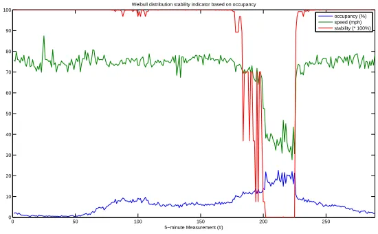
Based on the definition of metastability, a stochastic approach could be used. In this case, traffic flow is metastable as the probability of breakdown is larger than 0. The probability is based on historical data and uses the Product Limit Method of Kaplan & Meier (1958) and the Weibull distribution function (Appendix A). Drawback of this indicator is that it is assuming stationary and homogeneous flow. In other words; at a certain occupancy, in different situations, it will determine the same stability. Based on stationary and homogeneous flow, this indicator could be used to macroscopically measure whether traffic flow is in the metastable regime (regime where chance of breakdown larger than 0). The metastable regime is necessary for traffic control; as traffic has entered the metastable regime, a large perturbation can cause a breakdown. Therefore, this control could be used as it is giving a fixed value for the border of the metastable regime.

To overcome the drawback of the stochastic indicator, the reliability indicator of Ferrari (1988) could be used (Ferrari uses the word ’reliability’ for stability). Here, if a decrease in speed of a certain vehicle (in order to obtain a safe gap) can cause greater and greater decreases in the speed of the following vehicles, traffic flow is unstable (Ferrari, 1988). The indicator is based on the flow, the variance in flow and the (log normal) density (see Appendix A). It resolves the drawback of the stochastic stability indicator; the reliability indicator gives different values in different situations with the same demand. The stochastic approach could be used whether traffic has entered the metastable regime (based on historical data) and the reliability indicator could be used to measure the stability of traffic based on instationary flow. Here, this indicator could be used for more local traffic control as local ramp metering (section 5.1).

Note that both indicators should only be used for indicating stability in (uncontrolled) free flow.

3.5

Conclusion

4

Traffic Control

Previous chapter has shown that congestion on a highway is caused by a combination of high traffic flow, spatial inhomogenity and a temporary perturbation. To make sure the bottleneck will not be activated (and capacity will not drop) traffic can be controlled. Basically, the outflow of traffic can be improved using ramp metering, speed limits, route guidance, dedicated lanes (e.g. lane for high-occupancy vehicles), peak lanes, bi-directional lanes and by applying ’keep your lane’-signs. This report will only focus on two of these strategies; ramp metering and speed limits.

4.1

Traffic Control

4.1.1 Demand for Traffic Control

The increasing number of vehicles on the road has caused some serious congestion problems in the last decades. On a more local scale, the congestion forming at an active bottleneck causes a capacity drop and is blocking off-ramps. As discussed before, bottleneck activation leads to a drop in capacity. This is caused by accelerating vehicles from lower speeds (within the congestion) to higher speeds (downstream of the bottleneck) (Carlson et al., 2010). Besides, the tail of the formed congestion propagates upstream (Papageorgiou & Kotsialos, 2000). It is possible that the congestion covers on- and off-ramps upstream of the bottleneck. Here, vehicles wanting to leave the mainline are also delayed due to the congestion and contribute to an accelerated spatial increase of the congestion (Carlson et al., 2010). One solution to solve these problems is constructing new roads; adding lanes to existing roads or creating alternative new highways, both expensive solutions. Dynamic traffic control (or management) is an alternative; increasing the efficiency of the traffic network without constructing new roads (Hegyi, 2004).

4.1.2 Traffic Control Objectives

Traffic control may be applied for one or several objectives. Increasing the efficiency of the traffic network by minimizing the total travel time of an individual (user optimum) or minimizing the network travel time (network optimum) is one of these objectives. Another objective of traffic control could be safety; as accidents are in some cases the cause of traffic jams, a safer network will cause higher flows. Besides, in the congested flows more accidents arises and therefore less congestion will increase safety. On the other hand, lower densities combined with low speeds influence safety positively (Hegyi, 2004). This can cause a conflict with the efficiency objective. As traffic jams are not always prevented, it is valuable for drivers when travel time is predictable (Hegyi, 2004). If travel time is predictable, the arrival time can be estimated and choosing the de-parture time is easier. A, more recently developed, objective is lowering (negative) environmental effects of traffic. Emissions of a vehicle are influenced by the status of a vehicle, the technology of a vehicle, infrastructure and external conditions (Zegeye et al., 2009). Emissions per hour increase if the average speed increase, which is conflicting with reducing congestion. This report will only focus on traffic control to enhance the efficiency of a highway, in order to decrease the travel time of individuals.

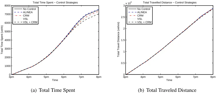
The efficiency of the network is measured by the total travel time of an individual or network. As this report is focusing on resolving congestion the network travel time needs to minimized. The total travel time in the network is formulated as the total time spent (TTS). The total (travel) time spent is the sum of the travel time of all vehicles between two fixed locations. The total travel time plus the total waiting time (time for vehicles waiting to enter the network) is the total time spent.

4.2. RAMP METERING 14

TTS is a variable to compare the performance of different control strategies, the lower the TTS the better the performance of the strategy. If the TTS is lower, vehicles spent less time between entering and leaving the network.

Another criterion used to estimate the efficiency performance is the total traveled distance (TTD). TTD reflects the total distance traveled by the vehicles between two points of time (note difference with TTS). If the TTD is higher at a certain time, vehicles were able to make more miles. Note, that in the a simulation environment the total traveled distance at the end of the simulation period is always the same, as no extra vehicles are able to enter the network. The ratio of the total distance covered by the total time spent gives the mean speed; as the total time spent can be minimized and the total traveled distance is maximized; the mean speed of all vehicles is maximized (in drivers’ perception: one can drive faster).

Although a strategy may perform better, still, it can show some undesired behavior. The strategy can cause new congestion areas and therefore the number of new traffic jams arisen should be identified empirically.

4.1.3 Principles of Traffic Control

The principles of traffic control are based on the three ingredients of congestion. As it is de-sired to prevent congestion, control is used to make sure the total flow is not exceeding capacity. Based on stability, it is desired to obtain a stable traffic flow. If traffic is stable, a disturbance will vanish without intervention. If traffic has entered the metastable regime, a large disturbance can cause congestion, the unstable regime indicates that any traffic disturbance will cause conges-tion. Therefore, if one wants to prevent traffic breakdown one should prevent traffic entering the unstable regime. If traffic has entered the metastable regime, control should be used to control perturbations.

4.2

Ramp Metering

To increase the performance of the network, several control strategies have been developed. Ramp metering is used to control the inflow of a ramp and based on occupancy; if the occupancy (lower than the critical occupancy) can be (approximately) continuous over time, no traffic jams will arise. Ramp metering can be implemented by installing traffic lights at the on-ramp of a highway, controlling the amount of traffic flow allowed to enter the highway (the ramp metering rate) (Figure 4.1). It can be used in order to increase or decrease travel time. When drivers try to bypass congestion on a highway it can be used to increase the travel time of these drivers (Middelham, 1999). Second, used in this report, a ramp metering strategy is used to preserve capacity flow on the mainstream and to avoid congestion (Kotsialos et al., 2002a). Referred is to Appendix B for more information about different ramp metering control strategies.

Basically, ramp metering strategies can be classified as static or dynamic, traffic responsive or feed forward, and local or coordinated (Hegyi, 2004). A fixed strategy, where the amount of vehicles allowed to enter the highway is based on historical demands, assumes, which is naive, that the demand is constant. This strategy is not able to adapt to variations in traffic (Hegyi et al., 2005). To overcome this (static) issue, the ramp metering strategy can be based on on-line data (traffic responsive strategy).

15 4. TRAFFIC CONTROL

ramp metering variable speed limits

50 55

Figure 4.1 Ramp metering and variable speed limits in order to control traffic (after Hegyi et al.

(2005)).

desired (occupancy) value. This strategy could be validated using traffic stability; as the desired value of occupancy lies in the stable regime congestion could be prevented. The summary of field results (Papageorgiou et al., 1997) shows that this traffic responsive strategy is outperforming other strategies, reducing travel time between 5 and 18 % and improving total traveled distance up to 3 %.

Local control strategies are focusing on controlling the ramp metering of a particular on-ramp. Coordinated ramp metering combines the use of several ramp meters to control the ramp flow on several on-ramps. Note that it is possible to (independently) control several ramps with a local con-trol strategy. It was shown (Papageorgiou et al., 1997) that a coordinated ramp metering strategy is more complex and in case of recurrent congestion is not better performing than ALINEA. This validates that the local ramp metering strategy ALINEA is a standard to which other strategies can be compared and therefore will be implemented in the simulation environment, and will be imple-mented in the simulation software. Simulation tests from Hegyi (2004), Carlson et al. (2010), Lu et al. (2011) and Bhouri et al. (2011) have shown that other coordinated ramp metering strategies are able to improve TTS performance up to 25 %, the TTD shows very little or no improvement (Bhouri et al., 2011; Lu et al., 2011). Concluded can be that coordinated ramp metering strategies have the potential to improve performance.

4.3

Variable Speed Limits

Nowadays, a lot of highways are equipped with variable speed limit signs. These signs are cur-rently used in The Netherlands to increase safety by lowering speed limits upstream of congested areas (Hegyi, 2004). Although, the signs could also be used to improve efficiency using a speed limit strategy.

Literature shows two approaches using speed limits; homogenization and preventing traffic break-down (Hegyi et al., 2005). The idea of homogenization is that speed limits can reduce differences in speed and density (and thus flow). A field test (Van den Hoogen & Smulders, 1994) has shown that capacity is not improved by this approach. The speed variations and number of very small gaps decreases using this approach. This could be validated by traffic stability; as the variance in gaps decreases and the flow is high, this would decrease the opportunity to change lanes (less large gaps available) and this will cause more imprudent lane changes triggering a breakdown. The reliability indicator (Ferrari, 1988) supports this statement. This is in contrast with the statement of Van den Hoogen & Smulders (1994) and Zackor (1991) that homogenization causes a more stable traffic flow and, thus, a higher capacity. This can be validated because Van den Hoogen & Smulders (1994) do not define stability and Zackor (1991) shows only a very small (negligible) increase of capacity.

4.4. CONCLUSION 16

speed limits lower than critical speed to limit the inflow of the bottleneck (Figure 4.1). Several speed limit strategies have been developed. The SPECIALIST (Hegyi et al., 2008) strategy is the only strategy applied in real world, used to resolve moving jams and showed a gain of travel time of 35 vehicle hours per resolved jam (Hegyi & Hoogendoorn, 2010). Drawback of this algorithm is that the detection of moving jams (relatively short jams with an upstream moving head and tail) requires high dense installed detectors. Strategies used to prevent or postpone traffic breakdown (sometimes in combination with coordinated ramp metering) use a predictive control method, optimizing an objective. The different simulation studies (Carlson et al., 2010; Lu et al., 2011; Hegyi et al., 2005) show an improvement of TTS up to 50 % and an improvement of TTD up to 35 %. These studies show that a combination of (coordinated) ramp metering and variable speed limits are able to further improve the TTS up to 55 % (Lu et al., 2011; Hegyi et al., 2005).

It is clear that a local ramp metering strategy and variable speed limit strategies (in combination with coordinated ramp metering) are able to improve travel time significantly. The literature shows that a strategy using variable speed limits in combination with coordinated ramp metering shows the best performance. Condition is that a speed limit approach focusing on preventing or resolving traffic breakdown is used.

4.4

Conclusion

5

Control Strategy based on Traffic

Stability

In the previous chapters is indicated that if traffic flow is entering the metastable regime, traffic needs to be controlled. In uncontrolled cases, disturbances can eventually lead to a breakdown. Traffic flow entering the metastable regime can be determined using historical traffic data. As the main objective of ramp metering and variable speed limits is preventing traffic breakdown, traffic may never enter the metastable regime. As the metastable regime has a significant lower flow than the capacity flow, it is undesired letting traffic flow never entering this regime. Besides, not every disturbance in the metastable regime will cause a breakdown. The desired control is, therefore, maximizing the flow in the metastable regime and controlling the disturbance to make sure the disturbances fade out. As in the previous chapter is shown that ramp metering strategies and variable speed limit strategies are able to improve the efficiency, here, these strategies are used for traffic control.

5.1

Local Ramp Metering Strategy

A local ramp metering strategy is able to improve the efficiency of a highway. It is able to control the inflow of the on-ramp and is therefore able to (temporary) prevent traffic breakdown. As the local ramp metering strategy is based on the total flow, it does not take into account the influence of a perturbation. According to Ferrari (1988), if traffic is unstable, vehicles further upstream will have a larger decrease in speed. This leads to an intuitive correction factor to the ramp meter rate Elbers (2005): if traffic flow is stable more vehicles are allowed to enter the highway. The cor-rection factor can be validated as the ramp metering strategy controls traffic based on the stability regime and the correction factor controls traffic based on the instationary stability (measured by the reliability indicator) of the flow:

rapplied(t) =rstrategy(t)∗c (5.1)

Here, rstrategy(t) is the ramp meter rate (number of allowed vehicles to pass the traffic light in

one hour) calculated by the local ramp metering strategy (based on stationary flow) at time step

t. The correction factor (c) is based on the instationary stability and gives the applied ramp meter raterapplied(t). Referred is to Appendix B for the calculation of the ramp meter rate by local and

coordinated ramp metering strategies.

Based on literature, it is suggested that the correction factor should be determined based on the following variables:

• Length on-ramp (fixed): Lee (2006) has shown that the gap acceptance is mainly influenced by the distance left to the end of the on-ramp. If the length of the on-ramp is small, vehicles will lower the gap acceptance more quick, which will lead to more disturbances. Lee (2006) has shown that more variables are influencing the gap acceptance, only the length of the on-ramp is introduced in this correction factor as Lee (2006) has shown that this is the major factor influencing the gap acceptance.

• Mainline shoulder lane flow (measured): if the mainline flow is increased, the variance in gaps increases and the average gap is lower (Vasconcelos et al., 2012; Brilon, 1988; Sullivan & Troutbeck, 1994); assuming that every vehicle will eventually make the mandatory lane change this is giving a higher probability of a serious disturbance.

5.2. INTEGRATED CONTROL 18

• Stability of the shoulder lane (indicated): if the flow is high and the stability of the traffic flow is also high, the chance that the disturbance will lead to a breakdown is low.

• Stability all the other lanes (indicated): if traffic is facing a merging vehicle (leaving the on-ramp) this indicates whether this vehicle is able to make a discretionary lane change (to the left), and so on.

• Number of vehicles passing the ramp meter (calculated): a ramp metering model (such as ALINEA) will calculate the number of vehicles entering the highway, Ahn & Cassidy (2007) indicated that a disturbance is amplified by another local disturbance.

• Speed at the shoulder lane (measured): if traffic flow has a high speed at the shoulder lane, lag vehicles will face a lower speed of the lane changing vehicle and the amplitude will be higher.

• Homogeneous traffic (measured): If a variable speed limit is active, the variance in gaps decreases. Literature has shown that this will decrease the capacity of the bottleneck, it was shown that the reliability indicator is able to adapt to this situation.

The mainline shoulder lane flow and the homogeneous traffic and their influence on the stability are already indicated using the stability indicator of Ferrari (1988). The total stability of the the flow upstream can be determined as follows:

Stability= 1

n

n X

i=1

φi (5.2)

Here,φi is the stability of lanei(Appendix A), andnis the number of lanes excluding a

desig-nated lane (HOV-lane). Mostly, desigdesig-nated lanes are not allowed to use by all vehicles and give, therefore, not the opportunity to change lanes to this designated lane. One must notice that the parameters of the reliability indicator should be changed as variable speed limit control is active. The correction factor has the following form:

c=β 1

n

n X

i=1

φi

+ (α1l−α2∆v) (5.3)

Here,lgives the length of the on-ramp, it is the length of the ramp entering the mainline and where this lane drops. ∆vgives the speed difference between the most right line (the merging lane) and the shoulder lane.

Where α1, α2 and β are control parameters. α2 has a negative sign as the speed difference is

negatively influencing the chance of a serious disturbance. Note that the ramp meter rate is based on measurements downstream of the on-ramp and the correction factor is based on measurements (stability) upstream of the on-ramp. Assuming that the measurements are made just upstream of the bottleneck, indicating that vehicles are only able to make a single lane change, stability will not change before facing the merging lane. The exact location of the detectors, influence of the variables and the control parameters is topic for further research before used as a control strat-egy. The performance of the strategy can, therefore, not be predicted. A, more simple, correction factor (Elbers, 2005) shows an improvement up to 15 % in total travel time in comparison with the ALINEA strategy. The correction factor of Elbers (2005) is based on microscopic measure-ments and is therefore not a proper indication of the performance of the proposed strategy in this section.

5.2

Integrated control

19 5. CONTROL STRATEGY BASED ON TRAFFIC STABILITY

a (simulation) improvement in total time spent up to 55 %. Therefore, an integrated strategy is proposed using both control strategies. To integrate these two control strategies three possible ways exist (Lu et al., 2011):

• Determine ramp metering rate before determining variable speed limits;

• Determine variable speed limits first before determining ramp metering rate;

• Determine ramp metering and variable speed limits simultaneously.

The third approach is more complex, a method for this strategy is proposed by Ghods et al. (2010), using a game theory approach. The first approach has some practical implications as highways already have implemented ramp meters (Lu et al., 2011). The second approach is used by Su et al. (2011) and Lu et al. (2011), showing an improvement of 55 % in total travel time. As this approach has shown it capability to improve the efficiency, it is used, here, as a starting point.

5.2.1 Speed Limit Design

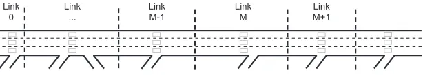
Assume a bottleneck on a highway caused by an on-ramp. Variable speed limits are able to limit the inflow of the mainline. As it is desired to differ the speed limit of different part of the highway (only a small section of the highway is a bottleneck and only the inflow needs to be controlled), the corridor is divided intoN links (m ∈ {0,1,2, . . . , N−1, N}). Each link has a set of loop detectors (for measurements), one on-ramp (as congestion is caused by a spatial inhomogenity) and may contain off-ramps. Although more loop detectors may be available in the corridor, the speed limit design does not use all these detectors for now. Assumed is that it is possible to set one speed limit per link.

Link ...

Link M-1

Link M

Link M+1 Link

0

Figure 5.1 Schematic corridor is divided intoN links, every link with one set of detector and an on-ramp. The link where the congestion is detected is linkM.

Here, the strategy is activated if traffic is approaching the metastable regime. This link is set as bottleneck linkMand will be controlled. In practice, the actual location of the bottleneck, caused by an on-ramp, is near the end of the on-ramp. Due to implementation reasons the entire link is set as bottleneck (Figure 5.1). Based on to the local ramp metering strategy ALINEA, the speed limit in the link upstream (M −1) of the bottleneck is based on the desired occupancy (oc) and

the measured occupancy (oˆ) (Su et al., 2011) in the bottleneck link. The set speed limitum(k)

is based on these variables and is a responsive strategy including a regulation parameter (ζ). The speed limit in the link upstream of the bottleneck can be calculated as new measurements are available from the loop detectors (everyT seconds). The time interval used iskT.

The equation used to set the speed limit in the link upstream of the bottleneck (M−1) is as follows (Su et al., 2011):

uM−1(k) =uM−1(k−1) +ζ(oc−oˆ(k−1)) (5.4)

5.2. INTEGRATED CONTROL 20

from upstream to downstream (see Figure 5.2). Assumed is that the most upstream link (m= 0) is in free flow and cannot be controlled (speed limits here could influence links outside of the considered section). Also, links downstream of the bottleneck and the bottleneck itself (m≥M) are not controlled by speed limits. The downstream links are not controlled as there is not demand for control (no approaching congestion detected), the bottleneck link is not controlled as only the inflow of the bottleneck (supply) needs to be controlled.

Figure 5.2 Schematic visualization of the variable speed limit strategy where the speed limit in a

linkmis gradually decreased up to the bottleneck linkM. Downstream links of the bottleneck, the most upstream link (m= 0) and the bottleneck link itself, are not controlled.

The following equation assumes that the speed limit in the upstream link is equal to the static speed limit (Vf) of the highway:

u0(k) =Vf (5.5)

The variable speed limit for each link is based on interpolation between the free flow speed (in

u0) and the speed in the link just upstream of the bottleneck. It can be determined as follows (Lu

et al., 2011):

um(k) =um−1(k) + max{−∆u,min{(ηαm(k) + (1−η)βm)[uM−1(t)−u0(k)],0}} (5.6)

Here, the maximum speed limit difference between two links is∆u(e.g.5mph). The speed limit in a link is, due to this equation, always lower or equal than the adjacent section upstream, and higher or equal than the section downstream. The speed limit in a section should be lower if the on-ramp demand (dm) is higher or if the on-ramp length Lm,o is lower. If on-ramp demand is

high, the speed limit should be lower to create more ’space’ for the on-ramp flow (Appendix B). Besides, if traffic is not able to leave the on-ramp a queue will grow and may be spill back to upstream adjacent infrastructure (outside of the network).

Therefore, Lu et al. (2011) and Su et al. (2011) have definedαandβ based on the length of the on-ramp, the fixed capacity (Qm) and the flow of the link (qm(k)).ηis used as a control parameter,

prioritizing the mainline or the on-ramp flow.

αm(k) =H(Qm−qm(k)) (5.7)

α causes a lower speed limit if the available ’space’ is low. β causes a lower speed limit if the on-ramp length is low:

21 5. CONTROL STRATEGY BASED ON TRAFFIC STABILITY

To allow more vehicles to be injected from the on-ramp the speed limit reduction at that link should be greater (Lu et al., 2011). Besides, if the available space is low on a link, the speed limit should be lowered. If the speed limit reduction is greater, would implicate that H is increased. The harmonic function calculates the ratio of a link based on all other controlled links. Letx₌

[x1, x2, . . . , xn]be a real vector, then (Su et al., 2011):

H(xm) =

1 x2

m

M−1 P

µ=1 1 x2

µ

(5.9)

Assume no ramp metering is active on the link. The flow leaving the on-ramp (Rm(k)) is restricted

by the demand of the ramp, capacity of the ramp (Qm,o) or ’space’ at the link (vehicles until

capacity) (Su et al., 2011). The ’space’ at a link is the capacity (Qm) of a link minus the net

measured inflow of the link (measured outflow of the upstream linkqˆm−1(k−1)). Here is assumed

that the off-ramp is located downstream of the on-ramp (within a link). This indicates that the ’space’ at the link is restricted by the mainline inflow and the capacity.

Rm(k) = min{dm(k), Qm,o, Qm−qˆm−1(k−1)} (5.10)

The expected flow of the link is the outflow from the previous link (measured:qˆm−1(k−1)) plus

the on-ramp flowRm(k)minus the off-ramp flowsm(k)(Lu et al., 2011). This indicates that the

speed limit in a link is updated based on the local (loop detectors) measurements.

qm(k) = ˆqm−1(k−1) +Rm(k)−sm(k) (5.11)

Here, as a link traffic is approaching the metastable regime, traffic can breakdown and needs to be controlled. The strategy bases the speed limit upstream of the bottleneck on the difference between the desired and the measured occupancy in the bottleneck link. However, the perturbations are not controlled and breakdown upstream of the bottleneck is still possible. To limit the chance of breakdown in a link, the ramp metering rate on a link should be controlled.

5.2.2 Optimal Ramp Meter Rate

After the variable speed limits are set in the links upstream of the bottleneck a model predictive control scheme is used to find the optimal ramp meter rate. Note that, without setting a speed limit, the predictive control can also be used (instead of speed limit the measured mean speed should be used).

Model Predictive Control

A model predictive control (MPC) scheme is used to find the optimal ramp metering rate (Cama-cho et al., 2004; Hegyi, 2004). The MPC controller (Figure 5.3) uses a linear traffic model and optimizes the control signal. This signal is applied to the traffic process (applied ramp metering rate) until new data is available. With the new data the signal is re-optimized with a shifted time horizon. In MPC, at each time step (every time new measurements are available), the optimal ramp meter rate is computed (using the simplex method) over a (finite) prediction horizonNp.

Assum-ing the inflows of the network are in the next time steps the same as the measurements, the MPC scheme calculates how many vehicles are allowed into the network to maximize the efficiency. As traffic situations change rapidly, only the ramp meter rate for the next time step is applied. In the next time step (k+ 1) a new optimization is performed, whereby the prediction horizon is shifted one step further, the so-called rolling horizon.

5.2. INTEGRATED CONTROL 22

conrol input: speed limits ramp metering

expected demand

traffi c demand

rolling horizon

(each k)

traffi c system

prediction

(N_p & N_c)

optimization

traffi c state:

speed fl ow density

control signals

perfor-mance controller

Figure 5.3 Schematic Model Predictive Control scheme, after Hegyi et al. (2005)

ramp meter rate until the control horizon Nc are used, other calculations are thrown away. Per

time step the following ramp meter rates are calculated, note that here the ramp metering is also applied in the bottleneck link (assuming the on-ramp is cause of the bottleneck).

r= [r1(k+ 1), . . . , r1(k+Np), . . . , rM(k+ 1), . . . , rM(k+Np)]T (5.12)

The predictive control takes irregular conditions into account, and the prediction is based (as will be shown in the next section) to predict traffic conditions if infrastructure changes. Thereby, the model predictive control makes frequent recalculations and therefore the control is updated frequently if traffic behaves different than expected (Schreiter, 2013).

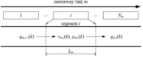
For the prediction of the traffic situation in the next time steps, the second order model METANET (Messner & Papageorgiou, 1990) is used. The motorway network is represented by a directed graph whereby the links of the graph represent motorway stretches with no on- or off-ramps and no major changes in geometry. Each link has all macroscopic characteristics (Figure 5.4):

• Traffic densityρm(k)(veh/mi/lane) is the number of vehicles in linkmat timekT divided

by the length of the linkLmand by the number of lanesλm.

• Mean speedvm(k)(mi/h) is the mean speed of the vehicles in linkm. In case of variable

speed limit, assumed to be equal to the calculated speed limit.

• Traffic flow qm(k)(veh/h) is the number of vehicles leaving linkm, divided byT (Loop

detectors give measurements per 20 or 30 seconds).

Figure 5.4 The original METANET (Messner & Papageorgiou, 1990) discretized motorway link,

after Kotsialos et al. (2002a).

23 5. CONTROL STRATEGY BASED ON TRAFFIC STABILITY

1971), where the density in the next time stepρm(k+ 1)is based on the current density (ρm(k)),

the inflow (qm−1(k)), the outflowqm(k), length of the on-ramp (Lm), number of lanesλmand the

time stepkT:

ρm(k+ 1) =ρm(k) +

T

Lmλm

(qm−1(k)−qm(k)) (5.13)

Adding an on- and off-ramp (respectively rm(k) andsm(k)) to this equation gives the

follow-ing:

ρm(k+ 1) =ρm(k) +

T

Lmλm

(qm−1(k)−qm(k) +rm(k)−sm(k)) (5.14)

The flow can be determined linear, therefore the density in the next time step is calculated as follows (Messner & Papageorgiou, 1990):

ρm(k+1) =ρm(k)+

T

Lmλm

(λmρm−1(k)um−1(k)−λmρm(k)um(k)+rm(k)−sm(k)) (5.15)

Clear is that the density in the next time step is a linear process, where the detector intervalT, length of the link Lm and the number of lanesλm are fixed values. Here, assumed is that the

speed limit in a linkum(k)is already calculated. The ramp metering rate are set as unknown and

will be set using the predictive control scheme.

Note that every link has detectors available. Each time step the macroscopic characteristics of a link at timekare, therefore, known. As each time step new measurements are available, the model is taking rapid changing traffic situations into account. Assumed is here that the loop detectors give information for the entire link.

The previous equations have determined the influence of the ramp metering rate on the mainline density. Besides influencing the mainline density, the ramp meter rate is also influencing the queue at an on-ramp.

The on-ramp demand (dm,o) at linkmis forwarded into the network. The queue at an on-ramp

is the old queue wm(k), the demand of the on-ramp (dm(k)) minus the on-ramp leaving flow

(qm,o). In case of ramp metering rate, the on-ramp leaving flow is the ramp meter rate (Messner &

Papageorgiou, 1990).

wm(k+ 1) =wm(k) +T[dm(k)−qm,o(k)] (5.16)

Due to this linear model, the macroscopic characteristics of the highway can be calculated. The unknown variables are the ramp meter rates for all the links until the prediction horizon. The optimal ramp metering rate will be calculated using an objective function.

Objective Function

As the goal of the strategy is to maximize performance, the total time spent needs to be minimized and the total traveled distance needs to be maximized. First, to obtain the optimal ramp metering rate the total time spent, in all speed limit sections and the bottleneck, need to be minimized. Due to this optimization function the ramp metering rate is set such that vehicles spend as little as possible time on the highway. Here it is important to also take the time delay due to on-ramp queue into account; this is the number of vehicles waiting times the time interval. Minimizing this value minimizes the total time spent and avoids all traffic waiting at the on-ramp (Lu et al., 2011; Hegyi, 2004; Hegyi et al., 2005; Carlson et al., 2010).

T T S=T

Np

X

j=1 M X

m=1

Lmλmρm(k+j) +T

Np

X

j=1 M X

m=1

5.2. INTEGRATED CONTROL 24

The total traveled distance should be maximized as to maximize the link flow (Lu et al., 2011):

T T D=T

Np

X

j=1 M X

m=1

Lmλmqm(k+j) (5.18)

The optimization problem becomes (Su et al., 2011; Lu et al., 2011):

minJ =T T S−σT T D (5.19)

Whereσis a factor to balance the TTS en TTD.

Constraints

The designed ramp meter rate needs to satisfy a set of (technical) constraints to avoid unrealistic and undesired situations:

• The queue length may not exceed the length of the on-ramp. Here formulated as: the number of waiting vehicles may not exceed the maximum possible vehicles on the on-ramp (length times maximum density) :

0≤wm(k+j)≤Lm,oρJ

• The ramp meter rate should not be higher than the ramp demand (dm(k)), ramp capacity

(Qm,o) or space available in the mainline (this validates equation 5.16) (Lu et al., 2011):

0≤rm(k)≤min{dm(k), Qm,o, λmQm−qˆm−1(k)}

• The density in a section may not exceed the jam density (unrealistic situation):

0≤ρm(k)≤ρJ

Algorithm

The proposed strategy assumes a bottleneck linkM, the location of this bottleneck is based on the detection of congestion. The strategy is more adaptive for non-recurrent congestion (e.g. acci-dents) if it is dynamic (no fixed bottleneck locationM. An algorithm is developed:

1. Congestion detection: After measurements, test whether a the occupancy is exceeding a threshold (based on metastability or intuitive value).If several links are congested, pick the most downstream area. If the control strategy is already active and still congested, go to step 2. If no congestion is detected, wait for next measurements.

2. Set Variable Speed Limits: Based on the occupancy of the bottleneck link, set the speed limits upstream of the bottleneck. For application of the control scheme it is necessary that there are enough links upstream available for control. As the maximum speed limits between two links is set as∆u, indicating that the minimum speed limit in linkM −1is

max ={umin,(umax−(M−1)∆u)}. Go to step 3.

3. Set Ramp Meter Rate: Based on Model Predictive Control and the linear density dynamics, set the ramp meter rate for the links upstream of the bottleneck as well as for the bottleneck link itself. Apply the speed limits and the ramp metering rate, go to step 1.

Using this algorithm, allows the designer of the strategy to select the following tuning parame-ters:

• ostart,mthreshold which switches the control on/off, could be different per link and is based

on the metastability principle.