Factors in the Paid-Incurred
Chain Reserving Method
by Michael Merz and Mario V. Wüthrich
AbSTRACT
In many applied claims reserving problems in P&C insurance,
the claims settlement process goes beyond the latest
devel-opment period available in the observed claims develdevel-opment
triangle. This makes it necessary to estimate so-called tail
development factors which account for the unobserved part of
the insurance claims. We estimate these tail development
fac-tors in a mathematically consistent way. This paper is a
modi-fication of the paid-incurred chain (PIC) reserving model of
Merz and Wüthrich (2010). This modification then allows for
the prediction of the outstanding loss liabilities and the
cor-responding prediction uncertainty under the inclusion of tail
development factors.
KEYwORdS
Tail factors, claims reserving, paid-incurred chain, outstanding loss liabilities, PIC model, claims development triangle, ultimate claim prediction,
1. Introduction and
model assumptions
Often in P&C claims reserving problems, the claims settlement process goes beyond the latest development period available in the observed claims development triangle. This means that there is still an unobserved part of the insurance claims for which one needs to build claims reserves. In such situations, claims reserv-ing actuaries apply so-called tail development factors to the last column of the claims development triangle which account for the settlement that goes beyond this latest development period. Typically, one has only limited information for the estimation of such tail development factors. Therefore, various techniques are applied to estimate these tail development factors. Most of these estimation methods are ad hoc methods that do not fit into any stochastic modeling framework. Popular estimation techniques, for example, fit para-metric curves to the data using the right-hand corner of the claims development triangle (Mack 1999; Boor 2006; Verrall and Wüthrich 2012). In practice, one often does a simultaneous study of claims payments and claims incurred data, i.e., incurred-paid ratios are used to determine tail development factors (see Sec-tion 3 in Boor 2006).
In this paper we review the paid-incurred chain (PIC) reserving method. The log-normal PIC
reserv-ing model introduced in Merz and Wüthrich (2010) can easily be extended so that it allows for the inclu-sion of tail development factors in a natural and mathematically consistent way. Similar to common practice, the tail development factor estimates will then be based on incurred-paid ratios within our PIC reserving framework.
In the following, we denote accident years by i ∈
{0, . . . , J} and development years by j ∈ {0, . . . , J,
J+ 1}. Development year J refers to the latest observed
development year of accident year i = 0 and the step
from J to J + 1 refers to the tail development factors
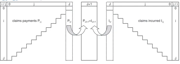
(see Figure 1). Cumulative payments in accident year
i after j development years are denoted by Pi, j and
the corresponding claims incurred by Ii, j. Moreover,
for the ultimate claim we assume Pi, J+1 = Ii, J+1 with
probability 1 (see Figure 1). This means that we assume that—after several development periods beyond the latest observed development year J—the cumulative payments and the claims incurred lead to the same ultimate claim amount. That is, ultimately,
when all claims of accident year i are settled, Ii, J+1 and
Pi, J+1 must coincide.
Model Assumptions 1.1 Log-normal PIC reserving model, Merz and Wüthrich (2010)
• Conditionally, given parameters Q = (F0, . . . ,
FJ+1, Y0, . . . , YJ, s0, . . . , sJ+1, t0, . . . , tJ), we have
i / j 0 j
J 1
+ J J
j 0
j / i
0 0
i claims payments Pi,j PiJ PiJ+1=IiJ+1 IiJ claims incurred Ii,j i
J J
Figure 1. PIC reserving model. Left panel: cumulative payments Pi,j development triangle;
– the random vector (x0,0, . . . , xJ,J+1, z0,0, . . . , zJ,J)
has a multivariate Gaussian distribution with uncorrelated components given by
xi, j~ N(Fj,s2j) for i ∈ {0, . . . , J} and
j∈ {0, . . . , J + 1}, and
zi, j~ N(Yj,t2j) for i ∈ {0, . . . , J} and
j∈ {0, . . . , J};
– cumulative payments Pi, j are given by the
recur-sion, j = 0, . . . , J + 1,
Pi, j= Pi, j-1 exp{xi, j}, with initial value Pi, -1= 1;
– claims incurred Ii, j are given by the (backwards)
recursion, j = 0, . . . , J,
Ii, j= Ii, j+1 exp{-zi, j},
with initial value Ii, J+1= Pi, J+1.
• The components of Q are independent and sj, tj > 0
for all j (with probability 1).
For an extended model discussion we refer to Merz and Wüthrich (2010). Basically, the PIC Model Assumptions 1.1 are a combination of Hertig’s (1985) log-normal model (applied to cumu-lative payments) and Gogol’s (1993) Bayesian claims reserving model (applied to claims incurred). In contrast to the PIC reserving model in Merz and Wüthrich (2010), we now add an extra development
period from J to J + 1. This is exactly the crucial
step that allows for the consideration of tail devel-opment factors and it leads to the study of incurred-paid ratios for the inclusion of such tail development factors.
The PIC Model Assumptions 1.1 may be criticized because of two restrictive assumptions. We briefly discuss how these can be relaxed.
• Assumption Pi,-1= 1 for all i ∈ {0, . . . , J}: If there are known (prior) differences between differ-ent acciddiffer-ent years i, this can easily be integrated by setting Pi,-1= vi with constants v0, . . . , vJ > 0 describing these prior differences.
• Independence between xi, j and zi, l: This is probably
the main weakness of the model. However, this
assumption can easily be relaxed in the spirit of Happ and Wüthrich (2013). To keep the analysis simple, we refrain from studying this more com-plex model in the present paper.
2. Estimation of tail
development factors
At time J one has observed data given by the set
DJ =
{
P Ii j,, i j, :i+ ≤j J, 0≤ ≤i J, 0≤ ≤j J}
, and one needs to predict the ultimate claim amountsPi, J+1 = Ii, J+1, conditional on these observations DJ.
On the one hand, this involves the calculation of
the conditional expectations E[Pi, J+1|DJ, Q] and,
on the other hand, it involves Bayesian inference
on the parameters Q, given DJ (see Theorems 2.4
and 3.4 in Merz and Wüthrich 2010). In this sec-tion we discuss how to modify the general out-line of Model Assumptions 1.1 to incorporate tail development estimation.
2.1. Ultimate claims prediction
conditional on parameters
We apply Model Assumptions 1.1 to the tail devel-opment factor estimation problem. Therefore, we need to specify the prior distribution of the parameter
vector Q.
Often, there is subjectivity in claims incurred data
Ii, j because the use of different claims adjusters with
different estimation methods and changing reserv-ing guidelines. Therefore, for the present set-up we have decided to consider claims incurred data
Ii, j only for the estimation of tail development
informative as to prior distributions specifying prior uncertainty in this expert judgment, similar to Verrall
and Wüthrich (2012).
Thus, assumptions (2.1)–(2.2) imply that there is
no systematic drift in {J* + 1, . . . J + 1}, and under
these assumptions we consider tail factor estimation under the restricted observations given by
D P I i j J k l J l J
D P I l J
J i j k l
J i j k l
{
}
{
}
= + ≤ + ≤ ≥
= ≥
* , : , , *
, : * .
, ,
, ,
∩
In this spirit, we consider all cumulative payment observations but only claims incurred observations from development year J* on. That is, only the claims
incurred Ii,j from the latest J - J* + 1 development
periods J*, J* + 1, . . . , J are used to estimate tail
development factors and the claims reserves. We define the following parameters
w
j J
v w
l J J
j m
m j
j m
m j
l J n
n l J
l J n
n l J
∑
∑
∑
∑
η = Φ = σ
= +
µ = η − Ψ = + τ
=
= =
+
= + =
and ,
for 0, . . . , 1,
and ,
for *, . . . , .
0
2 2
0
1
2 1
2 2
Moreover, we define the parameters
w w
v w j J J
j J
j
J j
j j
β =
−
− > =
= −
+ 0 for *, . . . , ,
0 for 0, . . . , * 1.
1
2 2
2 2
The following result shows that bj can be
inter-preted as the credibility weight for the claims incurred observations:
Theorem 2.1. Under Model Assumptions 1.1 we have, conditional onQ and D*J ,
E Pi J DJ Pi J i Ii J i
J i l l J i l
l J i J
l J i J
J i J i
∑
∑
{
}
[
]
(
)
(
)
Θ =
− β Φ + σ + β Ψ
+ −β− β−
− −
= − = − +
+ − −
, *
exp 1 2 .
, 1 ,
1 ,
2 1
1
The prediction based on incomplete claims incurred
data is done as follows. Assume there exists J* ∈
{0, . . . , J} such that with probability 1
J J
Ψ ≡ τ2 2, (2.1)
and if J* < J
J J J
J J J
τ = τ = = τ ≡ τ
Ψ = Ψ = = Ψ ≡ τ
+ −
+ −
. . . ,
. . . 2. (2.2)
* * 1 1
* * 1 1
2
Note that if J* = J we simply assume YJ ≡t2J / 2.
These assumptions imply that there is no substantial claims incurred development after claims develop-ment period J*, i.e., there is no systematic drift in the claims incurred development after J*. This is seen as
follows, for j ∈ {J*, . . . , J}
E E E
E
i j i j
j j
[
]
[
[
]
]
[
]
{
}
{
}
{
}
− ζ = − ζ Θ
= − Ψ + τ =
exp exp
exp 2 1.
, ,
2
This implies that on average the claims incurred prediction is correct (and we have only pure random
fluctuations around this prediction), i.e., for j ∈
{J* + 1, . . . , J + 1}
E I I I
I I i j i j i j
i j i j
(
j)
(
)
{ }
[
]
== τ −
−
− −
,
Vco exp 1 ,
, 1 , ,
, 1 , 1
2 1 2
where Vco() denotes the coefficient of variation.
The fact that we allow tJ to differ from t corresponds
to the difficulty that the tail development factor may cover several development years beyond the last observed column in the claims development triangle and therefore we may allow for standard deviation
parameters tJ > t for the development period from
J to J + 1 (possibly covering more than one period).
Remark. If there is expert judgment about a drift
term in the claims incurred development Ii,J*, . . . , Ii,J+1
payment development, the last line describes the claims incurred development, and the middle line describes the gap between the diagonal claims incurred and the diagonal claims payment observations.
In order to perform a Bayesian inference analysis on the parameters we need to specify the prior
distri-bution of Q.
Model Assumptions 2.2 PIC tail development factor model
We assume Model Assumptions 1.1 hold true with positive constants s0, . . . , sJ+1, tJ*= . . . =tJ-1= t,
YJ*= . . . =YJ-1= t2/2 and YJ = t2J/2. Moreover, it
holds
N s m J
m
(
m m)
{
}
Φ φ , 2 for ∈ 0, . . . , +1 ,
∼
with prior parameters fm∈R and sm > 0.
Under Model Assumptions 2.2 the posterior dis-tribution u(F|D*J) of F= (F0, . . . , FJ+1), given D*J,
is given by
u D l
s J D m m m m J J
∏
(
Φ)
∝ ( )Θ −(
Φ − φ)
= + exp 1 2 . * (2.3) * 2 2 0 1
This immediately implies the following theorem:
Theorem 2.3. Under Model Assumptions 2.2 the posterior u(F|D*J) of F is a multivariate Gaussian distribution with posterior mean (f0post, . . . , fJ+1) and posterior covariance matrix
S
(D*J). Define the pos-terior standard deviation bysj s J j j J
post
j j
=
(
−2+ − +(
)
−2)
−1 2 = +1 σ for 0, . . . , 1..
Then, the inverse covariance matrix
S
(D*J)-1 = (an,m)0 ≤ n, m ≤ J+1 is given byan m sn v w post
n m i i
i J
n m
n m J
∑
(
)
(
)
= { }+( ) ( ) − { } − = − = − ∧ − ≥ +1 1 .
,
2 2 2 1
* 1 1
, * 1
The posterior mean (f0post, . . . , fJ+1) is obtained by
D c c post
J post
J j
∑
(
)
(
φ0 , . . . ,φ+1)
′ =( )
∗ 0, . . . , +1 ′,post
post
For the conditional variance we obtain
Pi J DJ E Pi J DJ
J i l
l J i J
∑
{
}
(
)
[
]
(
)
(
)
Θ = Θ
− β σ −
+ +
− = − +
+
Var *, *,
exp 1 1 .
, 1 , 1
2
2 1 1
For i > J - J* there holds bJ-i= 0 and, therefore,
we obtain a purely claims payment based prediction [see also Hertig’s model (1985) presented in Sec-tion 2.1 of Merz and Wüthrich (2010)]
Pi J i l l
l J i J
∑
{
(
Φ + σ)
}
−
= − + +
exp 2 .
,
2 1
1
For i ≤ J - J* there holds bJ-i > 0 and, therefore,
we obtain a correction term to the purely claims pay-ment based prediction which is based on the claims incurred-paid ratio Ii, J-i /Pi, J-i, i.e., for a large incurred-paid ratio we get a higher expected ultimate claim as can be seen from
P I P I
P I
P
i J i i J i J i i J i J i i J i
i J i J i
i J i
i J i
J i J i =
{
(
− β)
+ β}
= β
− −β − β − − − − − − − −
− − exp 1 log log
exp log .
, 1 , , , , , ,
2.2. Parameter estimation,
the general case
The likelihood function of the restricted
obser-vations D*J is given by [see also (3.5) in Merz and
Wüthrich (2010)]
l P
P
v w v w
I P I I D j j j i j i j i J j j J
J i J i J i J i
i J J
J i J i
i J i
i J i i j
J j j J J j j i j i j
J
∏
∏
∏
∏
∏
(
)
( )Θ ∝
σ − σ Φ −
× − − −
µ − η −
× τ
−
τ Ψ +
− = − = − − − − = − − − − − = − − = − + 1 exp 1 2 log 1 exp 1 2 log 1 exp 1
2 log ,
* 2 , , 1 2 0 0
2 2 2 2
0 * , , 2 0 1 * 1 2 , , 1 2
where ∝ means that only relevant terms dependent on
(2005), then fjpost given in (2.4) corresponds to the
linear credibility estimator in more general models.
2.3. Parameter estimation,
special case
J
* =
J
We consider the special case J* = J, that is, only
the claims incurred observation I0,J is considered in
the tail development factor analysis. This immediately provides:
Corollary 2.5. Choose J* = J. Under Model
Assumptions 2.2, the posterior distribution u(F|D*J)
of F is a multivariate Gaussian distribution with
F0, . . . , FJ+1 being independent. For m ≤ J* = J the
posterior distribution of Fm is given by (2.4). The
posterior of FJ+1 is given by
ΦJ D J
post J
J
J J
J N
I P
+ { } + = + +
1 1 1
0
0 2
2
*
,
,
~ φ γ log τ
+ −
(
)
+ + + + −
1 1 1 1 1
1
γ φj J ,aJ ,J ,
with inverse variance given by
aJ+ J+ =sJ−+ + σ + τ
(
J+ J)
−
,
1, 1 1 2
1 2 2 1
and credibility weight given by
s J
J J J
(
)
γ =
+ σ + τ
+
+ +
1
1 .
1
1
2 2
1 2
This means that in the case J* = J we obtain a
credibility-weighted average between the prior tail
development factor fJ+1 and the observation log
I P
J
J .
0, 0,
Henceforth, in this case only the latest incurred-paid ratio is considered for the estimation of the tail development factor.
3. Posterior claims prediction
and prediction uncertainty
3.1. General case
In view of Theorems 2.1 and 2.3 we can now predict
the ultimate claim Pi,J+1, conditional on the restricted
observations D*J, under Model Assumptions 2.2.
with vector (c0, . . . , cJ+1) given by
c s
P P
v w
I P
i j
j
j j
i j
i j i
J j
J i J i i J j
J J
i J i
i J i
J j J
∑
∑
= φ +σ
+
−
+ τ + τ
{ }
− =
−
− −
= − + −
−
−
≥ +
1 log
1
log
2 1 .
2 2
,
, 1 0
2 2
1 *
, ,
2 2
* 1
Note that the last term in the definition of an,m and
in the definition of cj corresponds to the development
years in D*J where we have both claims payments and
claims incurred information. Theorem 2.3 immediately implies the following corollary:
Corollary 2.4. Under Model Assumptions 2.2 the posterior u(F|D*J) of F is a multivariate Gaussian distribution withF0, . . . , FJ*, (FJ*+1, . . . , FJ+1) being independent with
N s
j D j
post
j j j j j
post
J
(
(
) ( )
)
Φ { } φ = γ φ + − γ φ1 , 2 (2.4)
* ∼
for j ≤ J* and credibility weight and empirical mean
defined by
γ
σ φ
j
j j j
i j
i j J j
J j s J j
P P
= − +
− + + = − +
1 1
1 1
2 2 and log
,
,−− =
−
∑
=1 0
0 i J j
j J
for , . . . , *
Henceforth, Corollary 2.4 shows that for
develop-ment years j ≤ J* we obtain the well-known
credibil-ity weighted average between the prior mean fj and
the average observation fj. The case j > J* is more
involved: one basically obtains a weighted average
between the prior mean fj, the average observation fj,
and the incurred-paid ratios log Ii, J-i /Pi, J-i, i ≥ J - j + 1.
We obtain the following theorem:
Theorem 3.2. Under Model Assumptions 2.2 the conditional MSEP of the Bayesian predictor E[
S
iJ= 0
Pi,J+1|D*J] for the aggregate ultimate claim
S
iJ= 0 Pi,J+1 is given by
E P D
e
E P D E P D
P D i i J
J
J
e D e
i k J
i J J k J J
i J J i J
J i J k J i J J k i k J i l J i l J
∑
∑
∑
(
)
(
)
[
] [
]
= − × ( ) ( )( ) ( ) + =−β −β ′ Σ + −β Σ
≤ ≤
+ +
{ }
+ =
− − − + − + = − = − + σ+
msep * 1 . * * , 1 0
1 1 1 1
0 ,
, 1 , 1
, 1 * 0
1 * 1 1 1 2
3.2. Special case
J
* =
J
with
non-informative priors
We revisit the special case J* = J and we also assume
non-informative priors meaning that s2
j → ∞. In that
case we obtain that the posterior distributions of F0,
. . . , FJ+1 are independent Gaussian distributions with
N J j P P s J j
j D j
post j i j i j i J j j post j J
∑
( )
Φ φ = φ =
− + = σ − + { } − = − 1
1 log ,
1 , , , 1 0 2 2 * ∼
for j ≤ J, and
N I
P
s a
j D J
post J
J J
J post
J J J J
J
(
)
Φ φ = + τ
= = σ + τ
{ } + + + −+ + + log 2 , . 1 1 0, 0, 2 1 2 1, 1 1 1 2 2 * ∼
This implies for the ultimate claim prediction for i > 0
E P D P s
P f f
i J J i J i l
post l l
post
l J i J
i J i l
l J i J
J ult
∑
∏
[
]
= φ + σ +(
)
= ( ) + − = − + + − = − + + exp 2 2 *
ˆ ˆ , (3.1)
, 1 ,
2 2 1 1 , 1 1
with chain-ladder factors
f
J l
l l
post l
{
(
)
}
= φ + +
− + σ
ˆ exp 1 1
1 2 , (3.2)
2 Proposition 3.1. Bayesian ultimate claims predictor.
Under Model Assumptions 2.2 we predict the ulti-mate claim Pi,J+1, given D*J, by
* exp
, , ,
E Pi J DJ Pi J i Ii J i
J i J i
+ − − − = − − − 1 1 1
β β β
JJ i
l
l J i J J i J i − = − + + −
(
)
+ + ×∑
σβ τ τ
2
1 1
2 2
2
2 expp 1
1 1 1 2 −
(
)
{
+ −(
)
′ − = − + + − −∑
β φ βJ i j
post
j J i J
J i J i
e ++
( )
− + ∑
1 1
2 D eJ J i
, *
where ej= (0, . . . , 0, 1, . . . , 1)′∈RJ+2 with the first j components equal to 0.
Next we determine the prediction uncertainty. Model Assumptions 2.2 and Theorem 2.3 consti-tute a full distributional model which allows for the calculation of any risk measure (using Monte Carlo simulations) under the posterior distribution, given
D*J. Here, we use the most popular measure for the
prediction uncertainty in claims reserving, the so-called conditional mean square error of prediction (MSEP). The conditional MSEP has the advantage that we can calculate it analytically. Analytical solu-tions have the advantage that they allow for more basic sensitivity analysis. The conditional MSEP is given by (see also Section 3.1 in Wüthrich and Merz (2008))
E P D
E P E P D D
P D
P i i J
J J i J i J i J i J J J i J i J J
i J DJ i J
∑
∑
∑
∑
∑
(
)
(
)
(
)
= − = + = + = = + + = + = msep * * *Var *,
, 1 0 , 1 0 , 1 0 2 , 1 0
, 1 * 0
i.e., in this Bayesian setup the conditional MSEP is equal to the posterior variance. This posterior vari-ance allows for the usual decoupling into average processes error and average parameter estimation error; see (A.3). The conditional MSEP satisfies
Pi J D P P D i
J
J i J k J J
i k J
∑
∑
(
+)
=(
)
= = + + *Var , 1 Cov , *.
0
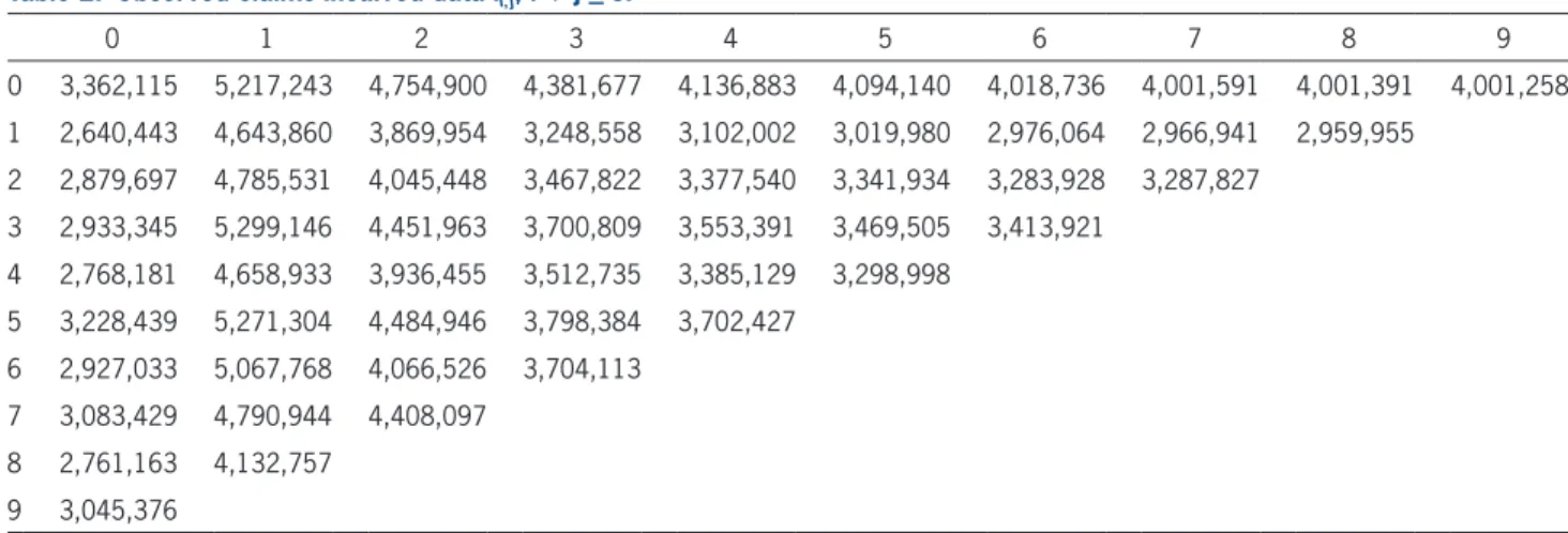
the claims incurred data Ii,j for i + j ≤ J are given by Tables 1 and 2, respectively.
We first need to determine J* ≤ J. We choose
the value J* such that there is no substantial claims incurred development (no systematic drift) after devel-opment period J*. This choice is made based on actu-arial judgment. We therefore look at the individual chain-ladder factors Ii,J+1/Ii,j, j ≥ 0 and i + j + 1 ≤ J. These are provided in Table 3. In the upper right tri-angle in Table 3 (with the individual chain ladder factors for years 6, 7, 8) we see no further systematic development, so we concentrate on possible choices J* ∈ {6, . . . , 9}.
The standard deviation parameters sj, sj and tj
should be determined with prior knowledge only. In our example we assume that we have non-
informative priors, which means that we set sj=∞.
For sj and tj we take an empirical Bayesian point of
f I P J
ult J
J
J J
{
}
= σ + τ
( )
+ +
ˆ exp . (3.3)
1 0 , 0 ,
1
2 2
That is, the first terms in the product on the right-hand side of (3.1) are the classical chain-ladder fac-tors for Hertig’s log-normal model (1985); see also (5.11)–(5.12) in Wüthrich and Merz (2008). The last term in (3.1), however, describes the tail development factor (adjusted for the variance).
For i = 0 we have
E PJ DJ P fJ J I ult
J J J
[
]
= ( ) ={
σ + τ}
+ * ˆ+ exp + . (3.4)
0 , 1 0 , 1 0 , 1
2 2
4. Example
In this section we provide an example. We assume
that J = 9 and that the claims payment data Pi,j and
Table 1. Observed claims payments data Pi, j, ij < J.
0 1 2 3 4 5 6 7 8 9
0 1,216,632 1,347,072 1,786,877 2,281,606 2,656,224 2,909,307 3,283,388 3,587,549 3,754,403 3,821,258 1 798,924 1,051,912 1,215,785 1,349,939 1,655,312 1,926,210 2,132,833 2,287,311 2,567,056
2 1,115,636 1,387,387 1,930,867 2,177,002 2,513,171 2,931,930 3,047,368 3,182,511 3 1,052,161 1,321,206 1,700,132 1,971,303 2,298,349 2,645,113 3,003,425
4 808,864 1,029,523 1,229,626 1,590,338 1,842,662 2,150,351 5 1,016,862 1,251,420 1,698,052 2,105,143 2,385,339
6 948,312 1,108,791 1,315,524 1,487,577 7 917,530 1,082,426 1,484,405
8 1,001,238 1,376,124 9 841,930
Table 2. Observed claims incurred data Ii, j, i j < J.
0 1 2 3 4 5 6 7 8 9
0 3,362,115 5,217,243 4,754,900 4,381,677 4,136,883 4,094,140 4,018,736 4,001,591 4,001,391 4,001,258 1 2,640,443 4,643,860 3,869,954 3,248,558 3,102,002 3,019,980 2,976,064 2,966,941 2,959,955
2 2,879,697 4,785,531 4,045,448 3,467,822 3,377,540 3,341,934 3,283,928 3,287,827 3 2,933,345 5,299,146 4,451,963 3,700,809 3,553,391 3,469,505 3,413,921
4 2,768,181 4,658,933 3,936,455 3,512,735 3,385,129 3,298,998 5 3,228,439 5,271,304 4,484,946 3,798,384 3,702,427
6 2,927,033 5,067,768 4,066,526 3,704,113 7 3,083,429 4,790,944 4,408,097
uncertainty in our model according to Proposition 3.1
and Theorem 3.2. We do this for J* ∈ {6, . . . , 9}. The
results are provided in Table 5.
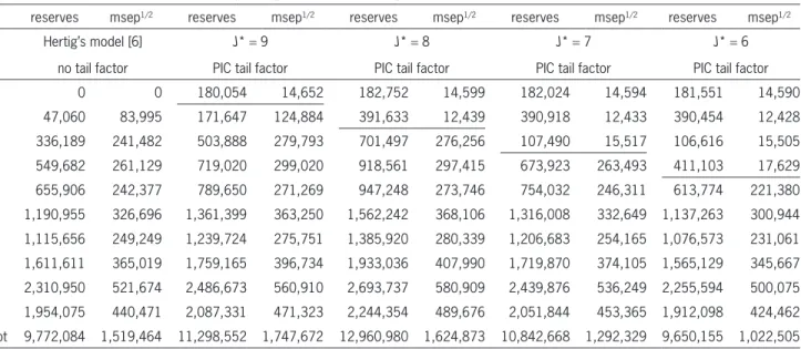
Interpretations
• The analysis shows that in the presence of tail development, Hertig’s model (1985) may sub-stantially underestimate the outstanding loss lia-bilities compared to the PIC tail development
factor models for J* = 9, 8, 7. Only the PIC tail
development factor model for J* = 6 gives
simi-lar reserves. This comes from the fact that the in-curred development factors still give a downward trend to incurred losses in development periods 6 and 7 (see average in Table 3), which contradicts our model assumptions (2.1)–(2.2) and suggests
to choose J* = 8 or 9. Of course, as mentioned
above, this expert choice is based on the ration-ale that there is no systematic drift after J*, and statistical methods could justify this hypothesis/ choice.
• Including tail development factors for J* = 8, 9
also gives a higher prediction uncertainty msep1/2
compared to Hertig’s model (1985) without tail development factors. This finding is in line with the
view and estimate them from the data. For j = 0, . . . ,
J- 1 we set
ˆ log , .
,
σj φ
i j
i j j i
J j
J j
P P
2
1 2
0
1
=
− −
− =
−
∑
Unfortunately, sJ and sJ+1 cannot be estimated from
the data, because we do not have sufficient observa-tions. Therefore, we make the ad hoc choice
J J
{
J J J J}
σ = σ =ˆ +1 ˆ min ˆ , ˆ , ˆσ −1 σ−2 σ−1 σˆ − . 2
2
We estimate the parameter t=t*J = . . . =tJ-1 with
the empirical standard deviation of log Ii,j+1/Ii,j for
i+ j + 1 ≤ J and j ≥ 6 (because we assume that there
is no systematic claims incurred development after
development period 6; see Table 3). Finally, for tJ
we do the ad hoc (expert) choice t2
J = 3t2. This
sug-gests that we have (approximately) another three
un-correlated development periods beyond J = 9 until all
claims are finally settled. Of course, additional
infor-mation about tJ (if available) should be used here.
These choices provide the standard deviation param-eters given in Table 4. Now we are ready to calculate the claims reserves and the corresponding prediction
Table 3. Individual chain ladder factors Ii, j1/Ii, j for j > 0 and i j 1< J.
0 1 2 3 4 5 6 7 8 9
0 1.5518 0.9114 0.9215 0.9441 0.9897 0.9816 0.9957 1.0000 1.0000 1 1.7587 0.8333 0.8394 0.9549 0.9736 0.9855 0.9969 0.9976
2 1.6618 0.8453 0.8572 0.9740 0.9895 0.9826 1.0012 3 1.8065 0.8401 0.8313 0.9602 0.9764 0.9840
4 1.6830 0.8449 0.8924 0.9637 0.9746 5 1.6328 0.8508 0.8469 0.9747
6 1.7314 0.8024 0.9109 7 1.5538 0.9201
8 1.4967 9
average 1.6529 0.8561 0.8714 0.9619 0.9807 0.9834 0.9980 0.9988 1.0000
Table 4. Estimated ˆj for j 0, . . . , J 1, and ˆj for j 6, . . . , J.
0 1 2 3 4 5 6 7 8 9 10
sˆj 0.1393 0.0650 0.0731 0.0640 0.0264 0.0271 0.0405 0.0227 0.0494 0.0227 0.0227
t
one given by D*J. In the present work we have
decided to work with the restricted information D*J
only because then we can fully concentrate on tail factor estimation. Otherwise tail factor estimation would be more hidden in the data and analysis.
5. Conclusion
We have modified the PIC reserving model from Merz and Wüthrich (2010) so that it allows for the incorporation of tail development factors. These tail development factors are estimated considering claims incurred-paid ratios in an appropriate way. This extends the ad hoc methods used in practice and because we perform our analysis in a mathe-matically consistent way we also obtain formulas for the prediction uncertainty. These are obtained analytically for the conditional MSEP and these can be obtained numerically for other uncertainty mea-sures using Monte Carlo simulations (because we work in a Bayesian setup). The case study highlights the need to incorporate tail development factors in the presence of tail development, since otherwise both the outstanding loss liabilities and the predic-tion uncertainty are underestimated.
ones in Verrall and Wüthrich (2012) and shows that prediction uncertainty needs a careful evaluation in the presence of tail development.
• Note that for J* = 9 we simultaneously consider
claims payments and claims incurred information
for accident year i = 0. For J* = 8 we
simultane-ously consider claims payments and claims
in-curred information for accident years i = 0, 1. This
results in a much lower prediction uncertainty in these accident years (above the horizontal line in the corresponding columns of Table 5). The reason is that the claims incurred information has only
lit-tle uncertainty (since we assume Yj to be constant
for j ≥ J*). This substantially reduces the
predic-tion uncertainty.
We may question whether there is so much infor-mation in these last claims incurred observations. If this is not the case, we should either increase
t and tJ or we should use less informative priors
in (2.1)–(2.2). The latter would bring us back to the model of Merz and Wüthrich (2010) and Happ and Wüthrich (2013) with the additional assump-tion that there is no systematic drift after J*. Moreover, this latter model would also allow us to consider more information than just the restricted
Table 5. Estimated claims reserves and corresponding prediction standard deviation in the PIC tail development factor model (Model Assumptions 2.2) for J* {6, . . . , 9}, and the estimated claims reserves according to Hertig’s model (1985)
[see Section 3.1 in Merz and Wüthrich (2010)] without tail development factor
reserves msep1/2 reserves msep1/2 reserves msep1/2 reserves msep1/2 reserves msep1/2
Hertig’s model [6] no tail factor
J* = 9 PIC tail factor
J* = 8 PIC tail factor
J* = 7 PIC tail factor
i≤ J - J*. We set j = J - i, then using Lemma A.1 we obtain completely analogous to Theorem 2.4 and Corollary 2.5 in Merz and Wüthrich (2010)
E P D
P I
w w
P I i J J
J j i j j j i j j
j J J
i j i j j l l j
l j J
l l j
J
j j
{
∑
∑
}
{
}
[
]
(
)(
)
(
)
(
)
(
)
(
)
(
)
Θ= η + − β − η + β − µ
+ − β −
= − β Φ + σ + β Ψ
+ + + −β β = + + = , *
exp 1 log log
1 2
exp 1 2 .
, 1
1 , ,
1 2 2 , 1 , 2 1 1
Analogously, Theorem 2.4 from Merz and Wüthrich (2010) implies for the variance
Pi J DJ E Pi J DJ
j l l j J
∑
{
}
[
]
(
)
(
Θ =)
Θ− β σ −
+ +
= + +
Var *, *,
exp 1 1 .
, 1 , 1
2
2 1 1
This proves the theorem.
Proof of Theorem 2.3 and Corollary 2.4. We first
write all the relevant terms of the likelihood of F,
given D*J. They are given by
u D s P P s P P
s v w
i I P J j j j j j i j i j i J j j J j j j j j i j i j i J j j J J J J J
J i J i i
J J
m
J i J i
i J i m J i
J
∑
∏
∑
∏
∏
∑
(
)
(
)
(
)
(
)
(
)
Φ∝ − Φ − φ −
σ Φ −
× − Φ − φ −
σ Φ −
× − Φ − φ
× − −
Φ − τ + τ − − = − = − = − = + + + + − − = − − − = − + + * exp 1 2 1 2 log exp 1 2 1 2 log exp 1 2 exp 1 2
2 log . (A.1)
2 2 2 , , 1 2 0 0 * 2 2 2 , , 1 2 0 * 1 1
2 1 1
2 2 2 0 * 2 2 , , 1 1 2
From this we easily see that the posterior
distribu-tion of F, given D*J, is again multivariate Gaussian
and there only remains to determine the posterior mean and covariance matrix. If we square out all
terms in (A.1) for obtaining the F2
j and the FjFn
terms, we find the covariance matrix
S
(D*J). First ofall, we observe that the development periods with
j≤ J* are all on the first line of (A.1) which proves
the independence statement on F0, . . . , FJ*, (FJ*+1,
A. Appendix: Proofs
In this appendix we prove all the statements. We start with a well-known result for multivariate Gauss-ian distributions, see, e.g., Appendix A in Posthuma et al. (2008) and Johnson and Wichern (1988):
Lemma A.1. Assume (X1, . . . , Xn)′ is multivariate
Gaussian distributed with mean (m1, . . . , mn)′ and
positive definite covariance matrix
S
. Then we havefor the conditional distribution:
X X Xn N m
∑
∑
X m∑
∑
∑
∑
(
)
(
)
+ − − { } ( ) ( ) − − , ,1 ,..., 1
2 2 2,2 1 1,2 2,1 2,2 1 1,2 1,1 2 ∼
where X(2)= (X
2, . . . , Xn)′ is multivariate Gaussian
with mean m(2)= (m
2, . . . , mn)′ and positive definite
covariance matrix
S
2,2,S
1,1 is the variance of X1 andS
1,2=S
2,1′ is the covariance vector between X1 and X(2).Proof of Theorem 2.1. We first consider the case i > J - J*, that is Ii,k∉ D*J for k = 0, . . . , J - i,
hence-forth for accident years i > J - J* we do not consider
claims incurred information. Using the conditional independence of accident years, given the
param-eters Q, we obtain
E P
[
i J,+1 DJ*,Θ =]
E P[
i J,+1 Pi,0, . . . ,Pi J,−1,Θ]
.Furthermore, i > J - J* implies bJ-i= 0. Therefore,
the claim follows from Model Assumptions 1.1, as in (2.2) in Merz and Wüthrich (2010), and because
bj= 0 for j < J*. Similarly, we obtain for the
condi-tional variance
Pi J DJ E Pi J DJ l l J i
J
∑
{ }
(
)
[
]
(
+ Θ =)
+ Θ σ −= − + +
* *
Var , 1 , , 1 , exp 1 .
2 2
1 1
The case i ≤ J - J* is more involved. Using again
the independence of accident years conditional on Q,
we obtain
E P
[
i J,+1DJ*,Θ =]
E P[
i J,+1Pi,0, . . . ,Pi J i,−,Ii J, *, . . . ,Ii J i,−,Θ]
,P I i
E D
i J i i J i J i
l J i
J
l J i J
J i l
l J i J
J
J i J i
∑
∑
{
}
{
}
(
)
(
)
= − β σ +β τ + τ
× − β Φ
− −β − β − − = − + + − = − + +
− − exp 1
2 2
exp 1 * .
, 1
,
2 2 2
1 1
1 1
From Theorem 2.3 we know that, given D*I, F=
(F0, . . . , FJ+1) has a posterior multivariate Gaussian
distribution with posterior mean (f0post, . . . , fJ+1) and
posterior covariance matrix
S
(D*J). Henceforth, theposterior distribution of
S
j=J-i+1 Fj is Gaussian withmean
S
j=J-i+1fjpost and variance e′J-i+1S
(D*J) eJ-i+1. Thisproves the proposition.
Proof of Theorem 3.2. We obtain with the tower property of conditional expectations
P P D E P P D D
E P D E P D D
i J k J J i J k J J J
i J J k J J J
[
]
[
] [
]
(
)
(
)
=(
Θ)
+ Θ Θ
+ + + +
+ +
Cov , * Cov , *, *
Cov *, , *, *. (A.3)
, 1 , 1 , 1 , 1
, 1 , 1
This is the usual decomposition into average pro-cess (co-)variance and average parameter error. The
first term in (A.3) is equal to 0 for i ≠ k, because
accident years i are independent, conditionally given
Q. Henceforth there remains the case i = k. Using
Theorems 2.1 and 2.3 we obtain
E P D D
E E P D D
P I i
E D
i J J J
i J J J J i l
l J i J
i J i i J i J i l J i J
l J i J
J i l
l J i J
J
J i l
l J i J
J i J i
∑
∑
∑
∑
{
}
(
)
{
}
{
}
{
}
(
)
[
]
[
]
[
]
(
)
(
)
(
)
(
)
(
)
(
)
Θ= Θ − β σ −
= − β σ + β τ + τ
× − β Φ
− β σ −
( )
+
+ −
= − + +
−−β β− − −
= − + + − = − + + − = − + + − −
Var *, *
, exp 1 1
* *
exp 1
exp 2 1 *
exp 1 1 .
, 1 , 1 2 2 1 1 , 2 1 ,
2 2 2 2
1 1 1 1 2 1 1
From Theorem 2.3 we know that, given D*I F=
(F0, . . . , FJ+1) has a posterior multivariate Gaussian
distribution with posterior mean (f0post, . . . , fJ+1) and
posterior covariance matrix
S
(D*J). Henceforth, theposterior distribution of
S
j=J-i+1Fj is Gaussian withmean
S
j=J-i+1fjpost and variance e′J-i+1S
(D*J)eJ-i+1. This implies for the first term (A.3)post
J+1
J+1
post
J+1
J+1
. . . , FJ+1). Moreover, we see for j ≤ J* that the
pos-terior variance of Fj, given D*J, is given by
sj s J j post
j j
(
(
)
)
= −2+ − + σ1 −2 −1 2,
which provides an,m for n, m = 0, . . . , J*. The
poste-rior mean is given by
s s P P j post j post j j j i j i j i J j
∑
( )
φ = φ +
σ − = − 1 log . 2 2 2 , , 1 0
Next, we square out all terms for j > J* to get the covariance matrix. We obtain
s J n v w s J n v w n n
n n m
n m J J
n J J
J i J i i J n J m
J J
n n
n J J
n n m i i
i J
n m
n m J J
∑
∑
∑
∑
∑
∑
(
)
(
)
+ − + σ Φ + Φ Φ −
= + − +
σ
Φ + Φ Φ −
( ) ( ) ( ) ( ) = + + = + + − − − = − + ∨ − + − = + + − = − ∧ − = + + 1 1 1 1 . 2 2 2 , * 1
1
* 1 1
2 2 1
1 1
*
2 2
* 1 1
2 2 2 1
* 1 1
, * 1 1
This provides an,m for n, m = J* + 1, . . . , J + 1.
The posterior mean is obtained by solving the
poste-rior maximum likelihood functions for Fj, j ≥ J* + 1.
They are given by
u D s P P i I P
v w a
J j j j j i j i j i J j
J i J i
i J i
J i J i i J j
J J
m j m m J J
∑
∑
∑
(
)
∂ Φ∂Φ = φ + σ
+
τ + τ +
− − Φ =
− = − − − − − = − + − = + + log 1 log *
2 log !
0. (A.2) 2 2 , , 1 0 2 2 , , 2 2 1 * , * 1 1
Henceforth, this implies
c cJ
∑
( )
DJ J(
+)
′ =(
Φ Φ ′)
− + * , . . . , , . . . , , 0 1 1 0 1
from which the claim follows.
Proof of Corollary 2.5. The corollary follows from
Theorem 2.3 and Corollary 2.4.
Proof of Proposition 3.1. From Theorem 2.1 we obtain
E P D E E P D D P I
E i D
i J J i J J J i J i i J i
J i l l J i
J
l J i J
J
J i J i
∑
{
[
]
}
[
]
[
]
(
)
(
)
= Θ =
− β Φ + σ + β τ + τ
+ + −β− β−
− − = − + + − − , * * *
exp 1 2
2 *
, 1 , 1 ,
E P D e D e
E P D e D e
i J J J i J i J J i
i J J J i J i J J i
J i l
l J i J
∑
∑
∑
} )
( {
(
{
}
)
[
]
[
]
(
)
( )
(
)
( )
(
)
+ − β ′ −
= − β ′
+ − β σ −
+ − − + − +
+ − − + − +
− = − +
+
exp 1 1
* *
exp 1
* *
1 1 .
, 1
2 2
1 1
, 1
2 2
1 1
2 1 1
This completes the proof.
References
Boor, J., “Estimating Tail Development Factors: What to Do When the Triangle Runs Out,” Casualty Actuarial Society
Forum, Winter 2006, pp. 345–390.
Bühlmann, H., and A. Gisler, A Course in Credibility Theory and
its Applications, New York: Springer, 2005.
Dahms, R., “A Loss Reserving Method for Incomplete Claim Data,” Bulletin of the Swiss Association of Actuaries 2008, pp. 127–148.
Gogol, D., “Using Expected Loss Ratios in Reserving,”
Insur-ance: Mathematics and Economics 12, 1993, pp. 297–299. Happ, S., and M. V. Wüthrich, “Paid-Incurred Chain Reserving
Method with Dependence Modeling,” ASTIN Bulletin 43, 2013, pp. 1–20.
Hertig, J., “A Statistical Approach to the IBNR-Reserves in Marine Insurance,” ASTIN Bulletin 15, 1985, pp. 171–183. Johnson, R. A., and D. W. Wichern, Applied Multivariate
Statis-tical Analysis (2nd ed.), Englewood Cliffs, NJ: Prentice-Hall, 1988.
Mack, T., “The Standard Error of Chain Ladder Reserve Esti-mates: Recursive Calculation and Inclusion of a Tail Factor,”
ASTIN Bulletin 29, 1999, pp. 361–366.
Merz, M., and M. V. Wüthrich, “Paid-Incurred Chain Claims Reserving Method,” Insurance: Mathematics and Economics 46, 2010, pp. 568–579.
Posthuma, B., E. A. Cator, W. Veerkamp, and E. W. van Zwet, “Combined Analysis of Paid and Incurred Losses,” Casualty Actuarial Society E-Forum, Fall 2008, pp. 272–293.
Verrall, R. J., and M. V. Wüthrich, “Reversible Jump Markov Chain Monte Carlo Method for Parameter Reduction in Claims Reserving,” North American Actuarial Journal 16, 2012, pp. 240–259.
Wüthrich, M. V., and M. Merz, Stochastic Claims Reserving
Methods in Insurance, Hoboken, NJ: Wiley, 2008.
E P D D E P D
e D e
i J J J i J J
J i J i J J i
J i l
l J i J
∑
∑
{
}
(
{
)
}
[
(
)
]
[
]
(
)
( )
(
)
Θ =
× − β ′
− β σ −
+ +
− − + − +
− = − +
+
Var ,* * *
exp 1 *
exp 1 1 .
, 1 , 1
2
2
1 1
2 1 1
Finally, we consider the last term in (A.3). Apply-ing Theorems 2.1 and 2.3, we obtain
E P D E P D D
P I i
P I k
D
i J J k J J J
i J i i J i J i
l
l J i J
J i
J
k J k k J k J k
l
l J k J
J k
J
J i l
l J i J
J k l
l J k J
J
J i J i
J k J k
∑
∑
∑
∑
{
}
{
}
{
}
(
{
} )
[
] [
]
(
)
(
)
(
)
(
)
(
)
Θ Θ
= − β σ +β τ + τ
× − β σ +β τ + τ
× − β Φ
− β Φ
+ +
− −β
− β
− = − +
+
−
− −β
− β
− = − +
+
−
− = − +
+
− = − +
+ − −
− −
Cov *, , *, *
exp 1
2 2
exp 1
2 2
Cov exp 1 ,
exp 1 *.
, 1 , 1
, 1
,
2
1
1 2 2
, 1
,
2
1
1 2 2
1 1
1 1
Henceforth, we need to calculate this last covari-ance term. Due to Theorem 2.3 the joint distribution of the exponents is a multivariate Gaussian distribution with covariance (1 -bJ-i)(1 -bJ-k) e′J-i+1
S
(D*J) eJ-k+1. This impliesCov E P D E P D D
E
i J,+ J*, , k J,+ J*, J*
(
)
=
1 Θ 1 Θ
P
Pi J D E PJ k J DJ
J i J
, * , *
exp
+ +
−
−
(
)
−1 1
1 β
(
1 β−−)
′− +( )
− +{
}
−(
k eJ i1∑
D e*J J k1 1 ,)
which is the well-known covariance formula for log-normal distributions. Collecting the terms for
i≠ k gives the off-diagonal terms. For i = k we obtain
the terms
E Pi J DJ J i eJ i D eJ J i
J i l
l J i J
∑
∑
{
}
(
)
{
}
[
]
(
)
( )
(
)
− β ′
− β σ −
+ − − + − +
− = − +
+
exp 1
* *
exp 1 1
, 1
2 2
1 1