Estimate
by Michael G. Wacek
ABSTRACT
This paper presents a framework for stochastically
mod-eling the path of the ultimate loss ratio estimate through
time from the inception of exposure to the payment of all
claims. The framework is illustrated using Hayne’s
log-normal loss development model, but the approach can be
used with other stochastic loss development models. The
behavior of chain ladder and Bornhuetter-Ferguson
esti-mates consistent with the assumptions of Hayne’s model
is examined. The general framework has application to the
quantification of the uncertainty in loss ratio estimates used
in reserving and pricing as well as to the evaluation of
risk-based capital requirements for solvency and underwriting
analysis.
KEYWORDS
1. Introduction
Ultimate loss ratio estimates change over time. The initial loss ratio estimate that emerges from the pricing analysis for a tranche of policies soon gives way to a new estimate as time passes and claims begin to emerge (or not). By the time all claims have been paid, the loss ratio is likely to have been re-estimated many times. The focus of this paper is on how to model the future re-visions of these ultimate loss ratio estimates. We illustrate the approach using loss ratio estimates based on chain ladder and Bornhuetter-Ferguson methods underpinned by a simple stochastic model described by Hayne [4].
There appears to be little, if any, actuarial lit-erature on the subject of behavior of an ultimate loss ratio estimate between the time when it is made and the time when its final value becomes known, i.e., the point at which all claims have been paid. Various authors have sought to ad-dress uncertainty in the ultimate loss ratio es-timate, but generally from the perspective of a single point in time.
For example, Hayne [4] proposed a lognormal model of loss development that supports the con-struction of confidence intervals around the ul-timate loss ratio esul-timate.1 Kelly [7] and Kreps [9] also used a lognormal framework to explore issues of parameter estimation and parameter un-certainty, respectively. Hodes, Feldblum, and Blumsohn [5] used a slightly different lognormal development model to quantify the uncertainty in workers compensation reserves. Mack, Ven-ter, and Zehnwirth have all written extensively about stochastic modeling of the loss develop-ment process.2 Others, including Van Kampen [12], Wacek [15], and the American Academy of Actuaries Property and Casualty Risk-Based
1Conscious that the confidence intervals he derived were dependent
on the lognormal model being the correct choice, he cautiously described his results as providing a “range of reasonableness.”
2For example, see Mack [10], [11], Venter [13], [14], and
Zehn-wirth [16], [2] (the last co-authored with Barnett).
Capital Task Force [1], have sought to quantify the uncertainty in the ultimate loss ratio estimate used in pricing and reserving applications di-rectly, without reference to the loss development process. The question on which all of these au-thors focused their attention is the potential vari-ation in the final loss ratio at ultimate compared to the current ultimate loss ratio estimate, with no reference to how the ultimate loss ratio estimate might vary at intermediate points in time.
In contrast, in his acclaimed paper on solvency measurement, Butsic [3] observed that loss esti-mates change in their march through time. He recognized that they, like stock prices, are gov-erned by a diffusion process, a type of contin-uous stochastic process with a time-dependent probability structure. However, he did not pro-pose a model of this stochastic process.
How ultimate loss ratio estimates change in the future depends in part on the method used to make the estimates. In this paper we assume that loss ratio estimates are derived from a con-sistently applied estimation process with mini-mal subjective overriding of the indicated result. We model the behavior of loss ratio estimates using stochastic versions of two loss develop-ment methods: the chain ladder method and the Bornhuetter-Ferguson method, both using paid development data. To model chain ladder esti-mates, we combine Hayne’s and Butsic’s ideas to synthesize a lognormal diffusion model for the path of the ultimate loss ratio. Then we adapt that model to the Bornhuetter-Ferguson method.
The paper comprises six sections, the first be-ing this introduction. In Section 2 we outline Hayne’s lognormal model of chain ladder loss development and illustrate its application using industry Private Passenger Auto Liability data from the 2004 Schedule P. We illustrate the main benefit of a stochastic model for loss develop-ment, namely, the ability to measure the uncer-tainty in loss development factors and in the ul-timate loss ratio esul-timate.
In Section 3 we discuss the effect of future loss emergence on future ultimate loss ratio esti-mates. We show how to use information implicit in Hayne’s model to determine the distribution of future estimates derived from our stochastic versions of the chain ladder and Bornhuetter-Ferguson methods, with particular attention to the loss ratio estimate one year out. We again use industry Private Passenger Auto Liability data to illustrate the process.
In Section 4 we adjust Hayne’s model to al-low for parameter uncertainty and illustrate the effect. Because the adjusted distribution does not have the multiplicative properties of the lognor-mal, we illustrate the use of Monte Carlo simula-tion to model the distribusimula-tion of future ultimate loss ratio estimates.
In Section 5 we conclude with an outline of potential applications of the framework for future ultimate loss ratio estimates in loss reserving and risk-based capital applications.
2. Hayne’s lognormal loss
development model
Hayne presented two models of chain ladder loss development: one that assumed that devel-opment is independent from one period to the next, and a second one that relaxed the indepen-dence assumption. We will adopt the first model (and henceforth refer to it simply as “Hayne’s model”). Kelly [7] argued that independence is more plausible for paid loss development than for case-incurred development. We will use paid
losses to illustrate our framework, but a good case can also be made for its application to ulti-mate loss ratio estiulti-mates based on case-incurred losses, even if all of the underlying assumptions are not always met.
Hayne’s model is quite simple. He assumed that age-to-age development factors are lognor-mally distributed. The product of independent lognormal random variables is also lognormal, which implies that age-to-ultimate loss develop-ment factors are lognormal. Because the product of a constant and a lognormal random variable is lognormal, if we are given the cumulative paid loss ratio at any age and the estimated param-eters of the matching age-to-ultimate factor, we can determine the parameter estimates of the ul-timate loss ratio. Using these parameters we can estimate the expected loss ratio (which we will take as the “best” estimate) as well as confidence intervals around that estimate.
The lognormal parameters¹and¾ of the age-to-age factors can be estimated by a variety of methods. Hayne used (and we also prefer) the unbiased estimators
¯ y= 1
n n
X
i=1
yi=1 n
n
X
i=1
ln(xi) and
s2= n
X
i=1
(yi¡y¯)2
n¡1
for ¹and ¾2, respectively, wherex1,x2,x3,: : :,xn are the observed age-to-age factors.3 y¯ is also a maximum likelihood estimator.
2.1. Illustration of model parameter
estimation
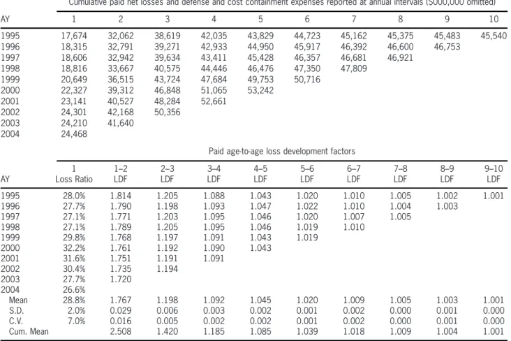
We illustrate the parameter estimation for Hayne’s model using the real loss development data presented in Tables 1 and 2. Table 1 shows
3We used unweighted unbiased estimators for¹and¾throughout
Table 1. Annual Statement for the year 2004 of the industry aggregate Schedule P, Part 3B, private passenger auto liability/medical
Cumulative paid net losses and defense and cost containment expenses reported at annual intervals ($000,000 omitted)
AY 1 2 3 4 5 6 7 8 9 10
1995 17,674 32,062 38,619 42,035 43,829 44,723 45,162 45,375 45,483 45,540
1996 18,315 32,791 39,271 42,933 44,950 45,917 46,392 46,600 46,753
1997 18,606 32,942 39,634 43,411 45,428 46,357 46,681 46,921
1998 18,816 33,667 40,575 44,446 46,476 47,350 47,809
1999 20,649 36,515 43,724 47,684 49,753 50,716
2000 22,327 39,312 46,848 51,065 53,242
2001 23,141 40,527 48,284 52,661
2002 24,301 42,168 50,356
2003 24,210 41,640
2004 24,468
Paid age-to-age loss development factors
1 1–2 2–3 3–4 4–5 5–6 6–7 7–8 8–9 9–10
AY Loss Ratio LDF LDF LDF LDF LDF LDF LDF LDF LDF
1995 28.0% 1.814 1.205 1.088 1.043 1.020 1.010 1.005 1.002 1.001
1996 27.7% 1.790 1.198 1.093 1.047 1.022 1.010 1.004 1.003
1997 27.1% 1.771 1.203 1.095 1.046 1.020 1.007 1.005
1998 27.1% 1.789 1.205 1.095 1.046 1.019 1.010
1999 29.8% 1.768 1.197 1.091 1.043 1.019
2000 32.2% 1.761 1.192 1.090 1.043
2001 31.6% 1.751 1.191 1.091
2002 30.4% 1.735 1.194
2003 27.7% 1.720
2004 26.6%
Mean 28.8% 1.767 1.198 1.092 1.045 1.020 1.009 1.005 1.003 1.001
S.D. 2.0% 0.029 0.006 0.003 0.002 0.001 0.002 0.000 0.001 0.000
C.V. 7.0% 0.016 0.005 0.002 0.002 0.001 0.002 0.000 0.001 0.000
Cum. Mean 2.508 1.420 1.185 1.085 1.039 1.018 1.009 1.004 1.001
Source: Highline Data LLC as reported in the statutory filings (OneSource)
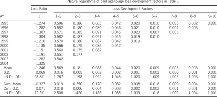
industry aggregate Schedule P net paid loss development data for Private Passenger Auto Liability for accident years 1995 through 2004 from the 2004 Annual Statement4 together with the associated paid loss age-to-age development factors. The paid loss ratios at age one year are also included in the development factor table. Ta-ble 2 shows the natural logarithms of the age-to-age factors and the age-to-age one year paid loss ratios. The rows labeled “Mean” and “S.D.” in Table 2 show the unbiased estimators for ¹ and ¾, re-spectively, given the data in the body of the column.5
4Source: Highline Data LLC as reported in the statutory filings
(OneSource).
5Note that the standard deviation for the age 9 to 10 development
factor, which is undefined, has been selected to be equal to that of the age 8 to 9 development factor in both Table 1 and Table 2.
For example, in Table 2 the mean and standard deviation of the natural logarithms of the ob-served age 1 to 2 development factors are 0.569 and 0.016, respectively. If we set ¹= 0:569 and ¾= 0:016,6 these parameter estimates for pro-spective age 1 to 2 development imply a log-normal mean, defined as E(x) = exp[¹+ 0:5¾2], of 1.767, which matches the mean loss develop-ment factor calculated by the traditional method in Table 1. The same is true for all of the other age-to-age factors. Similarly, the parameter esti-mates for the age one paid loss ratio are¡1:246 and 0.069 for¹and¾, respectively, which imply a lognormal mean of 28.8%. This, too, matches
6These parameters define the lognormal distribution that best fits
Table 2. Annual Statement for the year 2004 of the industry aggregate Schedule P, Part 3B, private passenger auto liability/medical
Natural logarithms of paid age-to-age loss development factors in Table 1
Loss Ratio Loss Development Factors
AY 1 1–2 2–3 3–4 4–5 5–6 6–7 7–8 8–9 9–10
1995 ¡1:274 0.596 0.186 0.085 0.042 0.020 0.010 0.005 0.002 0.001
1996 ¡1:282 0.582 0.180 0.089 0.046 0.021 0.010 0.004 0.003
1997 ¡1:307 0.571 0.185 0.091 0.045 0.020 0.007 0.005
1998 ¡1:304 0.582 0.187 0.091 0.045 0.019 0.010
1999 ¡1:210 0.570 0.180 0.087 0.042 0.019
2000 ¡1:135 0.566 0.175 0.086 0.042
2001 ¡1:151 0.560 0.175 0.087
2002 ¡1:191 0.551 0.177
2003 ¡1:282 0.542
2004 ¡1:325
Mean ¡1:246 0.569 0.181 0.088 0.044 0.020 0.009 0.005 0.003 0.001
S.D. 0.069 0.016 0.005 0.002 0.002 0.001 0.002 0.000 0.001 0.001
LN Fit LDFs 28.8% 1.767 1.198 1.092 1.045 1.020 1.009 1.005 1.003 1.001
Cum. Mean ¡0:327 0.919 0.350 0.170 0.082 0.038 0.018 0.009 0.004 0.001
Cum. S.D. 0.071 0.018 0.006 0.004 0.003 0.002 0.002 0.001 0.001 0.001
LN Fit LDFs 72.3% 2.508 1.420 1.185 1.085 1.039 1.018 1.009 1.004 1.001
Source: Highline Data LLC as reported in the statutory filings (OneSource)
the mean age one paid loss ratio shown in Ta-ble 1.7
The parameter estimates for the prospective age-to-age factors can be combined using the multiplicative property of lognormal distribu-tions to determine parameter estimates for pro-spective age-to-ultimate factors. The product ofn lognormal random variables with respective pa-rameter sets (¹1,¾1), (¹2,¾2), (¹3,¾3),: : :, (¹n,¾n) is a lognormal random variable with parameters
¹=
n
X
i=1
¹i and
¾=
à n X
i=1
¾i2
!1=2
:
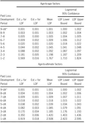
For example, treating age 10 as ultimate, in Ta-ble 2 the¹parameter estimate for the age 7 to ul-timate development factor is the sum of the mean age-to-age factor natural logarithms for ages 7 to 8, 8 to 9, and 9 to 10: 0:005 + 0:003 + 0:001 = 0:009. The corresponding ¾ parameter estimate
7We point this out to emphasize that the lognormal model appears
to fit this data well. However, it is important to note that the mean of the fitted lognormal does not necessarily equal the mean of the sample.
Table 3. Summary of estimated ultimate loss ratios from paid loss development analysis: private passenger auto liability, based on industry aggregate experience as of December 2004
Net Estimated
Accident Earned Net Paid Net Paid Age-to-Ult Ultimate Year Premiums Losses Loss Ratio Factor Loss Ratio
1995 63,183 45,540 72.1% 1.000 72.1% 1996 66,006 46,753 70.8% 1.001 70.9% 1997 68,764 46,921 68.2% 1.004 68.5% 1998 69,343 47,809 68.9% 1.009 69.6% 1999 69,231 50,716 73.3% 1.018 74.6% 2000 69,444 53,242 76.7% 1.039 79.6% 2001 73,143 52,661 72.0% 1.085 78.1% 2002 79,922 50,356 63.0% 1.185 74.6% 2003 87,242 41,640 47.7% 1.420 67.8% 2004 92,064 24,468 26.6% 2.508 66.7%
is the square root of the sum of the variances of the natural logarithms of the same age-to-age factors: p0:0002+ 0:0012+ 0:0012= 0:001.
Note that the lognormal means (labeled “LN Fit LDFs” in Table 2) implied by these age-to-ulti-mate parameters match the age-to-ultiage-to-ulti-mate de-velopment factors shown in Table 1.
lognor-Table 4. Summary of paid loss development factors with associated lognormal 95% confidence intervals: private passenger auto liability based on industry aggregate experience through December 2004
Age-to-age factors
Lognormal 95% Confidence Paid Loss
Development Est¹for Est¾for Mean LDF Lower LDF Upper
Period LDF LDF LDF Bound Bound
9–Ult* 0.001 0.001 1.001 1.000 1.002 8–9 0.003 0.001 1.003 1.002 1.004 7–8 0.005 0.000 1.005 1.004 1.005 6–7 0.009 0.002 1.009 1.006 1.012 5–6 0.020 0.001 1.020 1.018 1.022 4–5 0.044 0.002 1.045 1.041 1.048 3–4 0.088 0.002 1.092 1.087 1.097 2–3 0.181 0.005 1.198 1.187 1.209 1–2 0.569 0.016 1.767 1.710 1.824
Age-to-ultimate factors
Lognormal 95% Confidence Paid Loss
Development Est¹for Est¾for Mean LDF Lower LDF Upper
Period LDF LDF LDF Bound Bound
9–Ult* 0.001 0.001 1.001 1.000 1.002 8–Ult 0.004 0.001 1.004 1.002 1.006 7–Ult 0.009 0.001 1.009 1.007 1.011 6–Ult 0.018 0.002 1.018 1.015 1.022 5–Ult 0.038 0.002 1.039 1.034 1.043 4–Ult 0.082 0.003 1.085 1.079 1.091 3–Ult 0.170 0.004 1.185 1.176 1.193 2–Ult 0.350 0.006 1.420 1.403 1.436 1–Ult 0.919 0.018 2.508 2.423 2.595
*Age 10 deemed to be ultimate
mal loss development model produces the same loss ratio estimates as the traditional determinis-tic chain ladder loss development method. If we were interested only in these mean estimates, the traditional approach would suffice. However, we also want to measure the uncertainty in the loss ratio estimates, and for that purpose the richer lognormal model is superior.
2.2. Measurement of loss development
uncertainty
If we assume¹= ¯yand¾=sbased on the data for each age-to-age development period, we can calculate the lower and upper bounds of a two-sided 95% confidence interval for prospective age-to-age factors as exp[¯y¡N¡1(97:5%)¢s]
and exp[¯y+N¡1(97:5%)¢s], respectively, where N¡1(97:5%) is the value of the standard normal cdf corresponding to a cumulative probability of 97.5%.8 Similarly, using the parameter estimates for the age-to-ultimate factors, we can also de-termine confidence intervals for age-to-ultimate factors. We have tabulated these 95% confidence intervals based on the industry Private Passenger Auto Liability Schedule P data as of the end of 2004 in Table 4.9
Table 4 indicates that the age 1 to 2 devel-opment factor, which has an estimated mean of 1.767, should fall within a range of 1.710 to 1.824 95% of the time. The age 1 to ultimate de-velopment factor, which has an estimated mean of 2.508, can be expected to fall within a range of 2.423 to 2.595 95% of the time. Given the ac-cident year 2004 paid loss ratio of 26.6% at age 1, these confidence intervals imply a paid loss ra-tio range at age 2 of 45.5% to 48.5% (47:0%§ 1:5%) and an ultimate loss ratio range of 64.4% to 69.0% (66:7%§2:3%).10
As we would expect, the development factors for more mature accident years have tighter con-fidence intervals. For example, the age 5 to 6 factor, which in a year end 2004 analysis would be applicable to accident year 2000, has an es-timated mean of 1.020 and a 95% confidence range of 1.018 to 1.022, implying that 95% of the time the accident year 2000 paid loss ratio of 76.7% as of the end of 2004 will develop to a paid loss ratio of 78.1% to 78.4% by the end of 2005, a range of 0.3 points. The 95% con-fidence interval for the age 5 to ultimate factor,
8N¡1(97:5%) is replicated in Excel byNORMSINV(0.975). 9Bear in mind that these confidence intervals are premised on the
parameter estimates being correct and are narrower than confidence intervals that incorporate parameter uncertainty.
10While the lognormal is a skewed distribution, the skewness is
which has an estimated mean of 1.039, is a range of 1.034 to 1.043. That implies an ultimate loss ratio range of 79.3% to 80.0%, or 0.7 points.
All of these development factor, loss ratio, and confidence interval estimates are as of the end of 2004. They are all subject to change as new in-formation in the form of actual future loss emer-gence becomes available. In the next section we will show how to use information implicit in Hayne’s approach to model the effect of future loss emergence on these estimates.
3. A model for future ultimate loss
ratio estimates
Any estimate of the ultimate loss ratio for a particular accident year is quickly made obsolete by subsequent actual loss emergence. Because of this rapid obsolescence, the ultimate loss ratio must be re-estimated periodically in light of the loss development in the period since the previ-ous evaluation. That loss development affects the new estimate in two ways.
3.1. Sources of variation in future loss
ratio estimates
First, the actual accident year loss emergence replaces the expected emergence in the loss ratio projection. For example, in Table 3 the Private Passenger Auto Liability accident year 2004 ul-timate loss ratio of 66.7%, esul-timated as of the end of 2004, was determined by applying an age-to-ultimate factor of 2.508 to the paid loss ratio of 26.6%. That age-to-ultimate factor reflected an expected age 1 to 2 development factor of 1.767 combined with an age 2 to ultimate fac-tor of 1.420.
It is likely that actual age 1 to 2 loss devel-opment will vary from the expected. If, for ex-ample, the actual accident year 2004 emergence during 2005 (from age 1 to 2) corresponds to a development factor of 1.75, then in the ultimate loss ratio analysis conducted at the end of 2005 this actual development factor will replace the
expected development factor of 1.767. If the age 2 to ultimate factor remains unchanged at 1.420, the chain ladder estimate of the ultimate loss ratio will become 26:6%£1:75£1:42 = 66:1%. As-suming an expected ultimate loss ratio of 66.7%, the Bornhuetter-Ferguson loss ratio estimate will become 26:6%£(1:75¡1:767) + 26:6%£1:767 £1:42 = 66:1%.11,12
Of course, loss emergence with respect to older accident years might cause a revision in the pro-spective age 2 to ultimate factor. This potential for tail factor revision is a second source of un-certainty. For example, suppose the actual age 2 to 3 development on accident year 2003 during 2005 corresponds to a factor of 1.210. If that factor is averaged with the previous eight-point mean of 1.198 determined in Table 1 (using loss development data through 2004), the result is a revised age 2 to 3 development factor of 1.199. Assuming the same process is repeated for the other development periods, a revised age 2 to ultimate factor will be obtained. If the result-ing age 2 to ultimate factor is 1.425, the revised chain ladder ultimate loss ratio estimate is given by 26:6%£1:75£1:425 = 66:3%, a reduction of 0.4% from the year end 2004 ultimate loss ra-tio estimate of 66.7%. The revised Bornhuetter-Ferguson estimate in this case is given by 26:6%£(1:75¡1:767) + 26:6%£1:767£1:425 = 66:5%.
The foregoing is an illustration of just one sce-nario of the loss development that might occur in 2005 and its effect on the ultimate loss ratio estimate. We can use information developed in
11This is algebraically equivalent to the conventional statement of
the B-F estimate as Emerged LR + Expected Ultimate LR£(1¡1/ Ultimate LDF), which in this example would be expressed as 26:6%
£1:75 + 26:6£1:767£1:42£(1¡1=1:42). For the December 2005 valuation we will assume a B-F Expected Ultimate LR for each accident year equal to the corresponding chain ladder ulti-mate estiulti-mate as of December 2004 shown in Table 3. There are various ways to choose B-F Expected Ultimate LRs and ours may not be the one most commonly used in practice.
12Note that it is merely a coincidence that the chain ladder and B-F
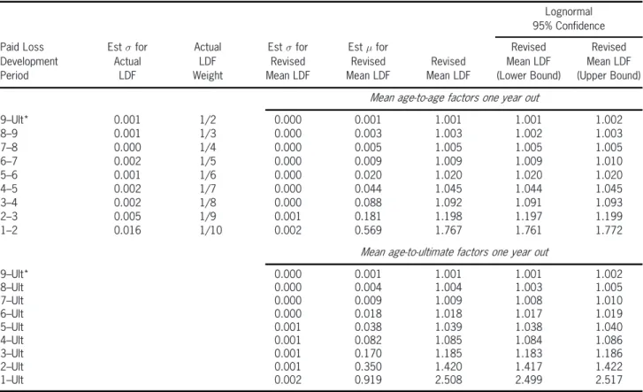
Table 5. Summary of revised mean paid loss development factors one year out: private passenger auto liability, based on industry aggregate experience through December 2004
Lognormal 95% Confidence
Paid Loss Est¾for Actual Est¾for Est¹for Revised Revised
Development Actual LDF Revised Revised Revised Mean LDF Mean LDF
Period LDF Weight Mean LDF Mean LDF Mean LDF (Lower Bound) (Upper Bound)
Mean age-to-age factors one year out
9–Ult* 0.001 1/2 0.000 0.001 1.001 1.001 1.002
8–9 0.001 1/3 0.000 0.003 1.003 1.002 1.003
7–8 0.000 1/4 0.000 0.005 1.005 1.005 1.005
6–7 0.002 1/5 0.000 0.009 1.009 1.009 1.010
5–6 0.001 1/6 0.000 0.020 1.020 1.020 1.020
4–5 0.002 1/7 0.000 0.044 1.045 1.044 1.045
3–4 0.002 1/8 0.000 0.088 1.092 1.091 1.093
2–3 0.005 1/9 0.001 0.181 1.198 1.197 1.199
1–2 0.016 1/10 0.002 0.569 1.767 1.761 1.772
Mean age-to-ultimate factors one year out
9–Ult* 0.000 0.001 1.001 1.001 1.002
8–Ult 0.000 0.004 1.004 1.003 1.005
7–Ult 0.000 0.009 1.009 1.008 1.010
6–Ult 0.000 0.018 1.018 1.017 1.019
5–Ult 0.001 0.038 1.039 1.038 1.040
4–Ult 0.001 0.082 1.085 1.084 1.086
3–Ult 0.001 0.170 1.185 1.183 1.186
2–Ult 0.001 0.350 1.420 1.417 1.422
1–Ult 0.002 0.919 2.508 2.499 2.517
*Age 10 deemed to be ultimate
Hayne’s framework to model these two effects generally.
3.2. Modeling the first source of
variation—Accident year development
The first effect is captured by the lognormal random variable estimated for the next year of development with respect to the accident year under review. For example, for accident year 2004, which at the end of 2004 is age 1, the lognormal distribution with ¹= 0:569 and ¾= 0:016 models age 1 to 2 paid development. Then, since the age 1 paid loss ratio is 26.6%, the paid loss ratio distribution at age 2 is lognormal with parameters ¹= ln 26:6% + 0:569 =¡0:756 and ¾= 0:016, implying a mean of 47.0%.
If the mean age 2 to ultimate factor (the tail factor) of 1.42 does not change, then the distribu-tion of the revised chain ladder ultimate loss ratio estimate at age 2 (i.e., one year out) has
lognor-mal parameters¹= ln 26:6% + 0:569 + ln 1:42 = ¡0:406 and ¾= 0:016. The random variable for this chain ladder estimate xCL can be expressed as a function of the paid loss ratio random vari-able xP and the expected value of the mean tail factor:
xCL=xP¢E(tail) (3.1)
The random variable xBF for the comparable Bornhuetter-Ferguson estimate is a shifted ver-sion of the random variable for the age 2 paid loss ratio:
xBF=xP¡E(xP) +E(xP)¢E(tail) (3.2)
3.3. Modeling the second source of
variation—Tail factor revision
The second effect, due to tail factor revision, is captured by measuring the effect of the log-normal loss development modeled for the next year on the existing mean age and age-to-ultimate factors. For example, the mean age 2 to 3 development factor shown in Table 1 is 1.198. This is a mean of eight data points. What will be the effect on the mean of adding a ninth data point (representing 2005 development on acci-dent year 2003), given that it will arise from a lognormal distribution with parameters¹= 0:181 and ¾= 0:005 (and mean of 1.198)? The uncer-tain ninth data point will contribute one-ninth weight to the revised mean age-to-age factor. There is no uncertainty about the existing mean age 2 to 3 factor–it is a constant. Therefore, the¾parameter of the distribution of the revised mean age 2 to 3 factor one year out, given an additional year of actual development, is given byq(89 ¢0)2+ (1
9¢0:005)2= 0:001. The¹
param-eter is given by ln 1:198¡0:5¢0:0012= 0:181.
We can use the same process to estimate ¹ and ¾ parameters for the comparable distributions of mean age-to-age factors one year out for all such factors comprising the development tail.13 We can then combine the revised mean age-to-age factor parameters to determine the parameters of the revised mean age-to-ultimate factor distribu-tions. See Table 5 for a tabulation of the parame-ters of these revised mean age and age-to-ultimate distributions for all ages. The ¾ of the distributions of revised factors for age 3 to 4 and beyond is less than 0.0005 (and thus displayed as 0.000 in Table 5), indicating that for Private Passenger Auto Liability, the uncertainty arising from the potential for tail factor revision is very
13Bear in mind that these parameters refer to distributions of the meanage-to-age development factor one year out and not to dis-tributions of the development factor itself. We are interested in the distribution of the mean development factor because changes in the mean directly affect the ultimate loss ratio estimate (which is also a mean).
small. This is confirmed by the very narrow con-fidences intervals.
3.4. Modeling the revised loss ratio
estimate one year out
We can now combine these two effects to de-termine the distribution of the revised ultimate loss ratio estimate that will be determined in one year’s time based on the updated loss develop-ment experience that will then be available.
To determine the distribution of the revised chain ladder estimate, we start with the actual accident year paid loss ratio, which we then mul-tiply by the lognormal random variables for (1) the age-to-age factor for the next year of devel-opment (obtaining the random variablexP of the paid loss ratio one year out) and (2) the revised age-to-ultimate factor beyond the next year of development. Using accident year 2004 as an ex-ample, as of the end of 2004 the ultimate loss ra-tio estimate is 66.7%, which has been determined by multiplying the paid loss ratio of 26.6% first by an age 1 to 2 factor of 1.767 and then by an age 2 to ultimate factor of 1.420. In order to model the ultimate loss ratio estimate one year later, at the end of 2005, we replace the con-stant age 1 to 2 factor of 1.767 with the lognor-mal random variable with parameters¹1= 0:569 and ¾1= 0:016. In addition, we replace the con-stant age-to-ultimate factor of 1.420 with the log-normal random variable with parameters ¹2= 0:350 and ¾2= 0:001. The expected values of these two lognormal random variables are 1.767 and 1.420, respectively. The product of the paid loss ratio (a constant) and these two log-normal random variables is loglog-normal with pa-rameters ¹= lnP+¹1+¹2 and ¾=q¾2
1+¾22,
where P represents the actual paid loss ratio at the end of 2004, which, in this example, implies ¹=¡1:325 + 0:569 + 0:350 =¡0:406 and ¾= p
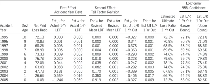
Table 6. Analysis of estimated ultimate loss ratios (chain ladder) one year out: private passenger auto liability, based on industry aggregate experience through December 2004
Lognormal
First Effect Second Effect 95% Confidence
Accident Year Devt Tail Factor Revision
Estimated Est L/R Est L/R Est¹for Est¾for Est¹for Est¾for Est¹for Est¾for Ultimate 1 Yr Out 1 Yr Out Accident Devt Net Paid Actual 1-Yr Actual 1-Yr Revised Revised Est Ult L/R Est Ult L/R Loss Ratio (Lower (Upper
Year Age Loss Ratio LDF LDF Mean LDF Mean LDF 1 Yr Out 1 Yr Out 1 Yr Out Bound) Bound)
1995 10 72.1% 0.000 0.000 0.000 0.000 ¡0:327 0.000 72.1% 72.1% 72.1%
1996 9 70.8% 0.001 0.001 0.000 0.000 ¡0:344 0.001 70.9% 70.8% 71.0%
1997 8 68.2% 0.003 0.001 0.001 0.000 ¡0:378 0.001 68.5% 68.4% 68.6%
1998 7 68.9% 0.005 0.000 0.004 0.000 ¡0:363 0.001 69.6% 69.5% 69.6%
1999 6 73.3% 0.009 0.002 0.009 0.000 ¡0:293 0.002 74.6% 74.4% 74.8%
2000 5 76.7% 0.020 0.001 0.018 0.000 ¡0:228 0.001 79.6% 79.5% 79.8%
2001 4 72.0% 0.044 0.002 0.038 0.001 ¡0:247 0.002 78.1% 77.8% 78.4%
2002 3 63.0% 0.088 0.002 0.082 0.001 ¡0:292 0.003 74.6% 74.3% 75.0%
2003 2 47.7% 0.181 0.005 0.170 0.001 ¡0:389 0.005 67.8% 67.1% 68.4%
2004 1 26.6% 0.569 0.016 0.350 0.001 ¡0:406 0.017 66.7% 64.5% 68.8%
2005 0 0.0% ¡1:246 0.069 0.919 0.002 ¡0:327 0.069 72.3% 63.0% 82.6%
Generally, we can express the random variable xCL as the product of the two lognormal random variables xP and tail, representing the paid loss ratio one year out and the mean tail factor:
xCL=xP¢tail (3.3)
Now we are in a position to determine confi-dence intervals for the revised chain ladder ulti-mate loss ratio estiulti-mate at the end of 2005. The endpoints of the two-sided 95% confidence in-terval are given by exp[¹¡N¡1(97:5%)¢¾] and exp[¹+N¡1(97:5%)¢¾], which imply an esti-mated loss ratio range one year out for accident year 2004 of 64.5% to 68.8%, or approximately 66:7%§2:1%. Confidence intervals for ultimate loss ratio estimates one year out for the other accident years can be estimated in the same way and are tabulated together with those for accident year 2004 in Table 6.
To determine the distribution of the compa-rable revised Bornhuetter-Ferguson estimate, we replace the constant E(tail) in Formula 3.2 with the random variabletail:
xBF=xP¡E(xP) +E(xP)¢tail (3.4)
We can also determine confidence intervals for the revised Bornhuetter-Ferguson loss ratio esti-mate at the end of 2005. However, because the
sum of two lognormal random variables, in this casexP and tail, is not expressible in closed dis-tributional form, the confidence intervals must be estimated using Monte Carlo simulation. The results of a simulation involving 10, 000 trials are shown in Table 7. For each of the trials we randomly selected observations from the distri-butions of xP and tail, assuming independence, and combined them according to Formula 3.4 to arrive at a simulated Bornhuetter-Ferguson esti-mate. After tabulating the results of 10, 000 such trials, we determined the lower and upper bounds of the 95% confidence interval of the loss ra-tio estimate by identifying the 2.5 percentile and the 97.5 percentile of the trial values. Not sur-prisingly, the 95% confidence intervals for the revised Bornhuetter-Ferguson estimates are nar-rower in every case than the revised chain ladder estimates.
3.5. Modeling the revised loss ratio
estimate—Other time horizons
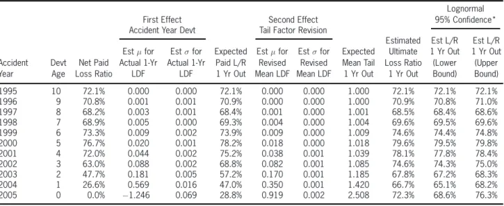
encom-Table 7. Analysis of estimated ultimate loss ratios (Bornhuetter-Ferguson) one year out: private passenger auto liability, based on industry aggregate experience through December 2004
Lognormal
First Effect Second Effect 95% Confidence*
Accident Year Devt Tail Factor Revision
Estimated Est L/R Est L/R Est¹for Est¾for Expected Est¹for Est¾for Expected Ultimate 1 Yr Out 1 Yr Out Accident Devt Net Paid Actual 1-Yr Actual 1-Yr Paid L/R Revised Revised Mean Tail Loss Ratio (Lower (Upper
Year Age Loss Ratio LDF LDF 1 Yr Out Mean LDF Mean LDF 1 Yr Out 1 Yr Out Bound) Bound)
1995 10 72.1% 0.000 0.000 72.1% 0.000 0.000 1.000 72.1% 72.1% 72.1%
1996 9 70.8% 0.001 0.001 70.9% 0.000 0.000 1.000 70.9% 70.8% 71.0%
1997 8 68.2% 0.003 0.001 68.4% 0.001 0.000 1.001 68.5% 68.4% 68.6%
1998 7 68.9% 0.005 0.000 69.3% 0.004 0.000 1.004 69.6% 69.5% 69.6%
1999 6 73.3% 0.009 0.002 73.9% 0.009 0.000 1.009 74.6% 74.4% 74.8%
2000 5 76.7% 0.020 0.001 78.2% 0.018 0.000 1.018 79.6% 79.5% 79.8%
2001 4 72.0% 0.044 0.002 75.2% 0.038 0.001 1.039 78.1% 77.8% 78.4%
2002 3 63.0% 0.088 0.002 68.8% 0.082 0.001 1.085 74.6% 74.3% 75.0%
2003 2 47.7% 0.181 0.005 57.2% 0.170 0.001 1.185 67.8% 67.2% 68.3%
2004 1 26.6% 0.569 0.016 47.0% 0.350 0.001 1.420 66.7% 65.1% 68.2%
2005 0 0.0% ¡1:246 0.069 28.8% 0.919 0.002 2.508 72.3% 68.6% 76.3%
*Based on Monte Carlo simulation ofxBF=xp¡E(xp) +E(xp)¢tail
passes the point when all claims are expected to have been settled. The modeling is conducted in essentially the same way as for the one-year time horizon. For example, in the case of a two-year horizon, the first source of uncertainty (accident year development) is modeled using the distri-bution of the age j to j+ 2 development factor, where j is the age in years of the accident year under review. The second source of uncertainty (potential tail factor revision) is modeled by ref-erence to the potential effect of two additional development data points on the mean tail fac-tor for age j+ 2 to ultimate development. The analysis of a three-year time horizon focuses on accident year development from age j to j+ 3 and the tail factor from j+ 3 to ultimate, but is otherwise identical to that for the one-year and two-year time horizons. The analysis of the ul-timate loss ratio esul-timate at points further in the future proceeds in the same way.
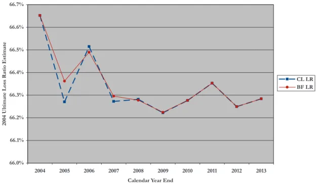
Alternatively, we can model the path of the ultimate loss ratio estimate as a succession of annual revaluations. Figure 1 illustrates this by plotting the results of one simulation of the path of the accident year 2004 loss ratio estimates through time for estimates determined from both
chain ladder and Bornhuetter-Ferguson methods. It represents just one path among many possibili-ties. The simulation was performed from the van-tage point of the end of 2004. As such, it incor-porates everything we know about actual loss de-velopment through that time as well as what we can infer about the structure of future develop-ment. We started with the accident year 2004 loss ratio estimate as of the end of 2004, which was 66.7%. Then, based on one random simulation of loss development during calendar year 2005, we made new chain ladder and Bornhuetter-Ferguson estimates of the ultimate loss ratio as of the end of 2005. We repeated the process for calendar years 2006 through 2013, using the sim-ulated cumulative loss development through each valuation date. Figure 1 is a plot of the results. A complete description of the probability structure of the path can be built up from a simulation in-volving a large number of random trials, or, in the chain ladder case, directly from the properties of the lognormal distribution.
Figure 1. One path of the accident year 2004 ultimate loss ratio estimate.
all claims have been settled), at least for Private Passenger Auto Liability.14 We see this in Ta-ble 8, the top half of which compares the 95% confidence intervals for the accident year 1995 through 2004 chain ladder loss ratio estimates one year out with confidence intervals for the ac-cident year loss ratio estimates over the ultimate time horizon. If we contrast the 95% confidence interval for accident year 2004 for the one-year horizon with the 95% confidence interval for the chain ladder loss ratio estimate over the ultimate time horizon, we can see that the contribution from the out years is dwarfed by the contribution from the next 12 months. The 95% confidence interval for the ultimate time horizon indicates a range for the accident year 2004 loss ratio of 66:7%§2:3%, which is barely wider than the range for just one year out. This is true not only for accident year 2004, but also holds for acci-dent years 1995 through 2003.
For example, the accident year 2003 confi-dence interval of approximately 67:8%§0:7%
14There might be value in doing so for other lines that display more
loss development variability.
Table 8. Lognormal confidence intervals—ultimate loss ratios for one year vs. ultimate time horizons: private passenger auto liability, based on industry aggregate experience through December 2004
95% Confidence Intervals— Chain Ladder Estimates Accident
Year Dec 2004 One-Year Horizon Ultimate Horizon
1995 72.1% 72.1% 72.1% 72.1% 72.1%
1996 70.9% 70.8% 71.0% 70.8% 71.0%
1997 68.5% 68.4% 68.6% 68.4% 68.6%
1998 69.6% 69.5% 69.6% 69.4% 69.7%
1999 74.6% 74.4% 74.8% 74.3% 74.8%
2000 79.6% 79.5% 79.8% 79.3% 80.0%
2001 78.1% 77.8% 78.4% 77.7% 78.5%
2002 74.6% 74.3% 75.0% 74.1% 75.2%
2003 67.8% 67.1% 68.4% 67.0% 68.6%
2004 66.7% 64.5% 68.8% 64.4% 69.0%
95% Confidence Intervals— B-F Estimates Accident
Year Dec 2004 One-Year Horizon Ultimate Horizon
1995 72.1% 72.1% 72.1% 72.1% 72.1%
1996 70.9% 70.8% 71.0% 70.8% 71.0%
1997 68.5% 68.4% 68.6% 68.4% 68.6%
1998 69.6% 69.5% 69.6% 69.4% 69.7%
1999 74.6% 74.4% 74.8% 74.3% 74.8%
2000 79.6% 79.5% 79.8% 79.3% 80.0%
2001 78.1% 77.8% 78.4% 77.7% 78.5%
2002 74.6% 74.3% 75.0% 74.1% 75.2%
2003 67.8% 67.2% 68.3% 67.0% 68.6%
2004 66.7% 65.1% 68.2% 64.4% 69.0%
66.0% 66.1% 66.2% 66.3% 66.4% 66.5% 66.6% 66.7%
2004 2005 2006 2007 2008 2009 2010 2011 2012 2013
Calendar Year End
2004 Ult
imat
e Loss R
at
io Est
imat
e
for a one-year time horizon is almost as wide as that for the time horizon to ultimate of 67:8%§ 0:8%. For all of the older accident years, the first year of future development accounts for more than half of the variation associated with the ul-timate time horizon.
This phenomenon is not confined to loss ra-tio estimates over short vs. longer time horizons. The same effect is also seen in other situations not related to insurance, where variability is a function of time. For example, given the common assumption that future stock price movements are lognormally distributed and independent, the 95% confidence interval for a stock price one year out, given constant annualized volatility of ¾= 20% and an expected value of $66.70, is $45.07 to $98.71, a range of $53.64. Assum-ing the same expected value of $66.70, the 95% confidence interval for the stock price two years out is $38.22 to $116.11, a range of $77.80. The confidence interval range for the one-year time horizon stock price is 69% of the price range for the two-year time horizon. The reason for the dis-proportionate impact of the first period is that the confidence interval is not a linear function of ¾ but rather of¾pt, wheretrepresents the time lag in years. In the case of chain ladder ultimate loss ratio estimation, where the age-to-age¾typically declines as the accident year ages, this effect can be even more pronounced.
Turning now to the Bornhuetter-Ferguson esti-mates, which are inherently less variable, the ef-fect is smaller but still evident. The bottom half of Table 8 compares the 95% confidence inter-vals for accident year 1995 through 2005 loss ratio estimates one year out with the confidence intervals for the loss ratio estimates over the ulti-mate time horizon. In the Private Passenger Auto Liability example considered here, the 95% con-fidence interval for the accident year 2004 loss ratio estimate is approximately 66:7%§1:6%, which is about two-thirds of the range of the con-fidence interval for estimates at the ultimate time
horizon. For all of the older accident years, as in the case of the chain ladder estimates, the first year of future development accounts for more than half of the variation associated with the ul-timate time horizon.
3.6. Modeling the loss ratio estimate at
inception
Up to this point we have focused on modeling the distribution of the ultimate loss ratio after losses have begun to emerge. However, there is no reason why we cannot extend essentially the same procedure backward to the inception of loss exposure at age 0. Indeed, the benefit of doing so is that we can obtain a complete model of the path of the ultimate loss ratio from inception to ultimate.
The main difference in the procedure is that the lognormal model for loss emergence between age 0 and 1 describes the behavior of the paid loss ratio rather than an age-to-age factor. The rest of the analysis is merely an application of Formula 3.3.
For example, assume for the sake of illustra-tion that the age 1 paid loss ratios in Table 1 are lognormally distributed and reflect “on level” adjustments to the accident year 2005 level. The mean age 1 paid loss ratio is 28.8%, which we can take as an estimate of the 2005 “on level” age 1 paid loss ratio. The unbiased estimates of the parameters of the lognormal distribution rep-resenting the paid loss ratio at age 1 are ¹= ¡1:246 and ¾= 0:069. These parameters imply a lognormal mean paid loss ratio of 28.8% that matches the sample mean. The age 1 to ultimate development factor of 2.508 implies an ultimate loss ratio estimate at inception of 72.3%.
Applying the lognormal multiplicative rule de-scribed in Section 2, the parameters of the log-normally distributed ultimate loss ratio (at the ultimate time horizon) are¹=¡1:246 + 0:919 = ¡0:327 and ¾=p0:0692+ 0:0182= 0:071,
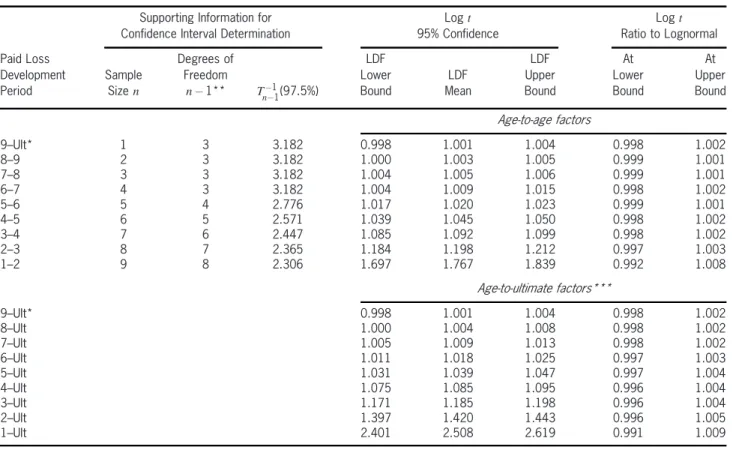
Table 9. Logtconfidence intervals for paid loss development factors reflecting parameter uncertainty: private passenger auto liability, based on industry aggregate experience through December 2004
Supporting Information for Logt Logt
Confidence Interval Determination 95% Confidence Ratio to Lognormal
Paid Loss Degrees of LDF LDF At At
Development Sample Freedom Lower LDF Upper Lower Upper
Period Sizen n¡1** Tn¡¡11(97.5%) Bound Mean Bound Bound Bound
Age-to-age factors
9–Ult* 1 3 3.182 0.998 1.001 1.004 0.998 1.002
8–9 2 3 3.182 1.000 1.003 1.005 0.999 1.001
7–8 3 3 3.182 1.004 1.005 1.006 0.999 1.001
6–7 4 3 3.182 1.004 1.009 1.015 0.998 1.002
5–6 5 4 2.776 1.017 1.020 1.023 0.999 1.001
4–5 6 5 2.571 1.039 1.045 1.050 0.998 1.002
3–4 7 6 2.447 1.085 1.092 1.099 0.998 1.002
2–3 8 7 2.365 1.184 1.198 1.212 0.997 1.003
1–2 9 8 2.306 1.697 1.767 1.839 0.992 1.008
Age-to-ultimate factors***
9–Ult* 0.998 1.001 1.004 0.998 1.002
8–Ult 1.000 1.004 1.008 0.998 1.002
7–Ult 1.005 1.009 1.013 0.998 1.002
6–Ult 1.011 1.018 1.025 0.997 1.003
5–Ult 1.031 1.039 1.047 0.997 1.004
4–Ult 1.075 1.085 1.095 0.996 1.004
3–Ult 1.171 1.185 1.198 0.996 1.004
2–Ult 1.397 1.420 1.443 0.996 1.005
1–Ult 2.401 2.508 2.619 0.991 1.009
* Age 10 deemed to be ultimate
** Judgmentally limited to a minimum of 3. (Variance not defined, if d.f.<3.) ***From Monte Carlo simulation (10,000 trials)
ultimate loss ratio one year out are ¹=¡1:246 +0:919 =¡0:327 and ¾=p0:0692+ 0:0022=
0:069. The indicated 95% confidence interval is 63.0% to 82.6%, a range of 19.6%. These calcu-lations are summarized in Table 6.
The comparable Bornhuetter-Ferguson esti-mate can be determined by applying Formula 3.4. Table 7 shows that the 95% confidence in-terval for the revised Bornhuetter-Ferguson es-timate of the accident year 2005 loss ratio one year out is 68.6% to 76.4%, a range of 7.8%.
4. Adjusting the model for
parameter uncertainty
In Section 2 we explained that, given the observations x1,x2,x3,: : :,xn arising from a log-normal process and the natural logarithms of the same observations y1,y2,y3,: : :,yn (where yi =
lnxi), the mean ¯yand standard deviation sof the log-transformed sample are unbiased estimators of the lognormal process parameters ¹ and ¾, respectively. The parameter selections ¹= ¯y and ¾=sdefine the lognormal distributionf(xj¹,¾) that best fits the data, using unbiasedness as the criterion for “best.”
However, while these are good estimates of the parameters, there is uncertainty about their true values. Fortunately, by combining informa-tion contained in the sample with results from sampling theory, it is possible to determine the mixed distributionf(x) that reflects the probabil-ity weighted contribution of all of the potential parameter values.15Wacek [15] showed thatf(x)
15This assumes that the historical data and future observations are
defines a “logt” distribution16 and in particular that the random variable y= lnx is Student’s t with n¡1 degrees of freedom, mean ¯y and vari-ance s2¢(n+ 1)=n¢(n¡1)=(n¡3).17
4.1. Log
t
confidence intervals
The bounds of the two-sided logt 95% confi-dence interval are given by exp[¯y¡Tn¡¡11(97:5%) ¢s¢p(n+ 1)=n] and exp[¯y+Tn¡¡11(97:5%)¢s¢
p
(n+ 1)=n], respectively, where Tn¡¡11(97.5%) is the value of the standard Student’s t cdf with n¡1 degrees of freedom corresponding to a cu-mulative probability of 97.5%.18 Two-sided 95% confidence intervals for Private Passenger Auto Liability age-to-age factors, based on the logt distribution, are shown in Table 9. Unfortunately, the logt distribution does not share the multi-plicative property of the lognormal. As a result, we cannot specify the distribution of age-to-ulti-mate development factors in closed form. In-stead, the age-to-ultimate factor distributions and related confidence intervals must be estimated using a Monte Carlo simulation procedure that determines the age-to-ultimate factor from the underlying age-to-age factors for each random trial.
In the top section of Table 9, we have tabulated the indicated logt 95% confidence intervals for age-to-age factors based on the industry Private Passenger Auto Liability 2004 Schedule P data, together with the ratios of these confidence inter-val bounds to the lognormal confidence interinter-val bounds given in Table 4. In addition, we have tabulated the sample size for each development period as well as Tn¡¡11(97.5%) and the degrees of freedom used in the calculations. At the risk of being seen as statistically less than rigorous, we set a minimum degrees of freedom value of
16The logtbears the same relationship to the Student’stdistribution
that the lognormal bears to the normal.
17Note that if we used the maximum likelihood estimators2
ml= Pn
i=1((yi¡y¯)2=n), the variance of this Student’s t distribution
could be expressed ass2
ml¢(n+ 1)=(n¡3).
18T¡1
n¡1(97.5)% is replicated in Excel byTINV(0:05,n¡1).
3 for purposes of calculating the confidence in-tervals to avoid using logt distributions with an undefined variance.
The logtconfidence intervals shown in Table 9 for age-to-age factors are very close to the log-normal confidence intervals given in Table 4. The largest difference is in the age 1 to 2 factor, where the upper bound of the logt interval is 1.839, which is only 0.8% larger than the lognormal up-per bound of 1.824. The up-percentage differences for the other age-to-age factors are smaller.
In the lower section of Table 9, we have tab-ulated the 95% confidence intervals for age-to-ultimate factors indicated by a Monte Carlo sim-ulation involving 10, 000 trials. As was the case with the age-to-age factors, the differences be-tween the logt confidence intervals and lognor-mal confidence intervals for the age-to-ultimate factors are quite small. For example, the largest difference is in the age 1 to ultimate confidence interval, where the upper bound of the logt in-terval is 2.619. This is only 0.9% larger than the lognormal upper bound of 2.595. The percentage differences for the other age-to-ultimate factors are smaller. This suggests that, at least for Private Passenger Auto Liability at the industry level, the effect of parameter uncertainty is small enough that it can be ignored. However, that is probably not the case for individual insurers, particularly small ones, writing Private Passenger Auto Lia-bility or for other lines of business.
4.2. Log
t
simulation of development
factors
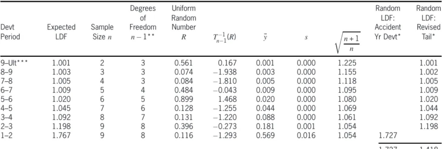
de-Table 10. Monte Carlo simulation of estimated ultimate loss ratio for accident year 2004 one year out: illustration of one random trial reflecting parameter uncertainty, private passenger auto liability, based on industry aggregate experience through December 2004
Degrees Uniform Random Random
of Random LDF: LDF:
Devt Expected Sample Freedom Number Accident Revised
Period LDF Sizen n¡1** R T¡1
n¡1(R) ¯y s Yr Devt* Tail*
r
n+ 1 n
9–Ult*** 1.001 2 3 0.561 0.167 0.001 0.000 1.225 1.001
8–9 1.003 3 3 0.074 ¡1:938 0.003 0.000 1.155 1.002
7–8 1.005 4 3 0.084 ¡1:810 0.005 0.000 1.118 1.005
6–7 1.009 5 4 0.484 ¡0:043 0.009 0.000 1.095 1.009
5–6 1.020 6 5 0.899 1.468 0.020 0.000 1.080 1.020
4–5 1.045 7 6 0.128 ¡1:255 0.044 0.000 1.069 1.044
3–4 1.092 8 7 0.131 ¡1:220 0.088 0.000 1.061 1.092
2–3 1.198 9 8 0.396 ¡0:273 0.181 0.001 1.054 1.198
1–2 1.767 9 8 0.116 ¡1:293 0.569 0.016 1.054 1.727
1.727 1.418
Revised Chain Ladder Loss Ratio Estimate One Year Out = Paid Loss Ratio x Actual Acc Year Devt x Revised Tail Factor = 26:6%£1:727£1:418 = 65:1%
Revised B-F L/R Loss Ratio Estimate One Year Out = Actual Paid L/R - Expected Paid L/R + Expected Paid L/R x Revised Tail Factor = (26:6%£1:727)¡(26:6%£1:767) + (26:6%£1:767)£1:418 = 65:6%
* = exp(¯y+T¡1
n¡1(R)¡s
p
(n+ 1)=n)
** Judgmentally limited to a minimum of 3. (Variance not defined, if d.f.<3.) ***Age 10 deemed to be ultimate
termined the lower and upper bounds of the 95% confidence interval for each age-to-ultimate fac-tor (age 1 to ultimate, age 2 to ultimate, etc.) by identifying the 2.5 percentile and the 97.5 per-centile of the 10, 000 trial values.
To make the random age-to-age factor selec-tions, we started with a random draw R from the uniform distribution defined on the interval [0, 1]. BecauseR has a value between 0 and 1, it can be treated as though it is a cumulative prob-ability. The number Tn¡¡11(R) that corresponds to a standard Student’s t cumulative probability of R is a random number from the standard Stu-dent’s t distribution with n¡1 degrees of free-dom, which has a mean of zero and a variance of (n¡1)=(n¡3). More generally, the correspond-ing random number from the Student’s t distri-bution with n¡1 degrees of freedom, mean M and varianceC2¢(n¡1)=(n¡3) is given byM+ Tn¡¡11(R)¢C, which corresponds to a random num-ber of exp[M+Tn¡¡11(R)¢C] from the related logt distribution. Substituting the appropriate values of ¯y for M and sp(n+ 1)=n for C, we obtain
exp[¯y+Tn¡¡11(R)¢sp(n+ 1)=n] as the value of a randomly selected age-to-age factor.
Putting some numbers to it, a draw of R= 0:873 implies a random age 1 to 2 development factor from the corresponding logt with 8 de-grees of freedom of exp(0:569 + 1:229¢0:016¢
p
10=9) = 1:803.19If the next draw isR= 0:239,
then the random age 2 to 3 factor, drawn from the corresponding logt with 7 degrees of freedom, is exp(0:181 + (¡0:749)¢0:005p9=8) = 1:194. Random numbers corresponding to the other development periods are similarly obtained. Then the age 1 to ultimate factor, the age 2 to ul-timate factor, age 3 to ulul-timate factor, and so on, are obtained by multiplication. Tabulation of these results completes the first trial. The pro-cess is repeated in the same way for 10, 000 trials.
19T¡1
n¡1(R) is replicated in Excel byTINV(2(1¡R),n¡1) ifR >
4.3. Log
t
simulation of future loss ratio
estimates
Under conditions of parameter uncertainty, the distribution of future loss ratio estimates must also be modeled using Monte Carlo simulation. Each of the lognormal age-to-age development components identified in Section 3 must be re-placed with corresponding logtcomponents.
For example, to estimate the distribution of the updated chain ladder estimate of the accident year 2004 ultimate loss ratio at the end of 2005, given the year-end 2004 estimate of 66.7%, we tabulated 10, 000 randomly obtained year-end 2005 loss ratio estimates. To determine each loss ratio estimate, we randomly selected from the logt distributions that represent the factors that contribute to the uncertainty in that estimate. For each trial we randomly selected one factor from the distribution of accident year 2004 develop-ment during 2005 and one factor from each of the age-to-age factor distributions that contribute to the revised tail factor. Then we multiplied all of these factors and the paid loss ratio as of year end 2004 to arrive at the ultimate loss ratio esti-mate for that trial.
This is illustrated in detail in Table 10 for one trial, where the simulated actual accident year 2004 age 1 to 2 development factor is 1.727 (compared to an expected factor of 1.767) and the revised tail factor is 1.418 (compared to an expected 1.420). The product of the year-end 2004 paid loss ratio and these two factors is the revised estimated ultimate loss ratio for accident year 2004 as of the end of 2005.
To arrive at approximate distributions of re-vised chain ladder ultimate loss ratio estimates for all of the accident years 1995 through 2004 as of the end of 2005, the process described in the preceding paragraph was repeated 10, 000 times for each accident year.20 The results of this
pro-20Note that largely because their tail factors overlap, the accident
year 1995 through 2004 ultimate loss ratio estimates are not in-dependent, and for that reason their distributions were modeled simultaneously. To give one example of the tail factor overlap, the
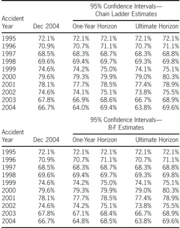
Table 11. Logtconfidence intervals—ultimate loss ratios, for one year vs. ultimate time horizons: private passenger auto liability, based on industry aggregate experience through December 2004
95% Confidence Intervals— Chain Ladder Estimates Accident
Year Dec 2004 One-Year Horizon Ultimate Horizon
1995 72.1% 72.1% 72.1% 72.1% 72.1%
1996 70.9% 70.7% 71.1% 70.7% 71.1%
1997 68.5% 68.3% 68.7% 68.3% 68.8%
1998 69.6% 69.4% 69.7% 69.3% 69.8%
1999 74.6% 74.2% 75.0% 74.1% 75.1%
2000 79.6% 79.3% 79.9% 79.0% 80.3%
2001 78.1% 77.7% 78.5% 77.4% 78.9%
2002 74.6% 74.1% 75.1% 73.8% 75.5%
2003 67.8% 66.9% 68.6% 66.7% 68.9%
2004 66.7% 64.0% 69.4% 63.8% 69.6%
95% Confidence Intervals— B-F Estimates Accident
Year Dec 2004 One-Year Horizon Ultimate Horizon
1995 72.1% 72.1% 72.1% 72.1% 72.1%
1996 70.9% 70.7% 71.1% 70.7% 71.1%
1997 68.5% 68.3% 68.7% 68.3% 68.8%
1998 69.6% 69.4% 69.7% 69.3% 69.8%
1999 74.6% 74.2% 75.0% 74.1% 75.1%
2000 79.6% 79.3% 79.9% 79.0% 80.3%
2001 78.1% 77.7% 78.5% 77.4% 78.9%
2002 74.6% 74.2% 75.1% 73.8% 75.5%
2003 67.8% 67.1% 68.4% 66.7% 68.9%
2004 66.7% 64.8% 68.5% 63.8% 69.6%
cess are summarized in Table 11, which, as the logtversion of Table 8, compares the 95% confi-dence intervals for the accident year 1995—2004 loss ratio estimates one year out with the con-fidence intervals for the estimates over the ul-timate time horizon. The chain ladder esul-timates are summarized in the top half of the table and the Bornhuetter-Ferguson estimates in the bot-tom half. As we observed in the lognormal case, much of the potential variation in the ultimate loss ratio estimates that is expected over the time horizon to ultimate is encompassed in the varia-tion expected over a one-year time horizon. For example, the logt 95% confidence interval for the chain ladder estimate of the accident year 2004 loss ratio one year out of 66:7%§2:7% is
nearly as wide as the 95% confidence interval of 66:7%§2:9% for the same loss ratio over the ul-timate time horizon. Similarly, the accident year 2003 confidence interval for the chain ladder es-timate of approximately 66:7%§0:9% for a one-year time horizon is also nearly as wide as that for the time horizon to ultimate of 67:8%§1:1%. For the older accident years, the proportion of the variation associated with the ultimate time hori-zon accounted for by the first year of future de-velopment is somewhat smaller, but the absolute size and significance of the confidence intervals for those years is much smaller.
Note that the logt confidence intervals are at least as wide in every case as the comparable lognormal confidence intervals shown in Table 7. In fact, in the case of the chain ladder estimates, for every accident year 1995—2004 the logt con-fidence intervals for the one-year time horizon are at least as wide as the lognormal confidence intervals for the ultimate time horizon!
5. Conclusions
There are a number of potential applications of the framework we have described for mod-eling future estimates of the ultimate loss ratio, ranging from loss reserving to pricing to analysis of risk-based capital. While a detailed discussion of these applications is beyond the scope of this paper, we will touch briefly on some examples.
5.1. Loss reserving
The framework presented in this paper gives reserve actuaries a way to manage their clients’ expectations. Reserve clients don’t like surprises and often express frustration that loss ratio or reserve estimates change significantly from one period to the next. We have shown in this pa-per that a large proportion of the potential vari-ation in ultimate estimates can be present in the first year of future development. As we saw in the Private Passenger Auto Liability example we
presented, this phenomenon is particularly pro-nounced when the estimates are determined us-ing the chain ladder method, but it can also be present if the estimates are derived from the Bornhuetter-Ferguson approach. It seems likely that most reserve clients do not understand this phenomenon. Actuaries have done a good job in getting clients to understand that ultimate loss estimates are subject to large potential variation, but many clients seem to expect that variation to emerge only in the distant future, if at all.
We suggest that the uncertainty in loss ratio and reserve estimates be framed in terms of how these estimates might change at the next valua-tion by presenting the ultimate estimates together with confidence intervals consistent with the val-uation time horizon. For example, if the next valuation will be in one year, then the results would be presented with one-year time horizon confidence intervals. Then, because the poten-tial variation has been explained to them in ad-vance, clients might be better able to accept the revised estimates produced at the next valuation. This framework also naturally facilitates the ex-planation of the reasons for estimate revisions in terms of the sources of variation. For example, how much of the revision is due to actual acci-dent year development and how much is due to a tail factor revision caused by loss emergence on the older accident years?
While we have focused much of our discussion on historical accident years and thus implicitly on reserving, we can easily extend this frame-work to encompass certain aspects of the pricing and underwriting, which can be used to assess risk load requirements and reinsurance risk trans-fer characteristics as well as to establish expec-tations for paid loss emergence during the first year after inception.
5.2. Risk-based capital
in his paper on solvency measurement in risk-based capital applications. He advocated the use of a common time horizon for measurement of all kinds of risks on both sides of the balance sheet. He showed how long-term solvency pro-tection could be achieved by periodic assessment and adjustment of risk-based capital using a short time horizon, e.g., one year. In particular, But-sic proposed that the risk-based capital charge at the beginning of each period be calibrated to a suitably small Expected Policyholder Deficit (EPD)21 expressed as a ratio to expected unpaid
losses. The capital charge would be reset at the beginning of each new period based on asset and/or liability changes during the period just ended. While he illustrated his approach with nu-merical examples, he did not describe a model for how claim liabilities change from one pe-riod to the next. The model presented in this paper, using parameters determined from Sched-ule P data, could be used together with Butsic’s approach to test and refine the capital charges employed in the NAIC and rating agency risk-based capital models.22 Moreover, to the extent that these risk-based capital charges imply the minimum amount of capital needed by an underwriter to assume risk, the model potentially has application to the problem of capital allocation for pricing applications as well.
5.3. Other stochastic loss development
models
We have used Hayne’s simple lognormal model to illustrate how to model the future be-havior of loss ratio estimates. However, the same
21The EPD is defined as the expectation of losses exceeding
avail-able assets. It can be viewed as the expected value of the proportion of policyholder claims that will be unrecoverable because of insurer insolvency.
22For stress testing these solvency models it may make sense to
use the chain ladder model, which produces more variable loss ratio estimates, rather than the Bornhuetter-Ferguson model.
conceptual approach can be used with other sto-chastic models. If ultimate loss ratios are esti-mated using a different stochastic model, the path of future revisions to those ultimate loss ratio estimates can be determined using the ideas pre-sented in this paper.
Abbreviations and notations
¹, first parameter of lognormal,E(¯y) =¹ ¾, second parameter of lognormal, E(s2) =¾2
EPD, expected policyholder deficit
f(xj¹,¾), distribution ofx, given known param-eters ¹,¾
f(x), distribution of x(unknown parameters) n, number of points in sample
N¡1(prob), standard normal inverse distribution function
P, actual paid loss ratio
R, random number from unit uniform distribu-tion
s, standard deviation of log-transformed sample Tn¡¡11(prob), standard student’s tinverse
distribu-tion funcdistribu-tion
tail, random variable for mean tail factor one year out
x1,x2,x3,: : :,xn, lognormal sample
xBF, Bornhuetter-Ferguson estimate of ultimate loss ratio
xCL, chain ladder estimate of ultimate loss ratio xP, cumulative paid loss ratio
y1,y2,y3,: : :,yn log-transformed sample ¯
y, mean of log-transformed sample
References
[1] American Academy of Actuaries Property/Casualty Risk-Based Capital Task Force, “Report on Reserve and Underwriting Risk Factors,” Casualty Actuar-ial Society Forum, Summer 1993, pp. 105—171, http://casact.org/pubs/forum/93sforum/93sf105.pdf. [2] Barnett, G., and B. Zehnwirth, “Best Estimates for
Reserves,”Proceedings of the Casualty Actuarial
So-ciety87, 2000, pp. 245—321, http://www.casact.org/
[3] Butsic, R. P., “Solvency Measurement for Property-Liability Risk-Based Capital Applications,” Casualty Actuarial Society Discussion Paper Program, 1992, pp. 311—354, http://www.casact.org/pubs/dpp/dpp92 /92dpp311.pdf.
[4] Hayne, R. M., “An Estimate of Statistical Varia-tion in Development Factor Methods,”Proceedings
of the Casualty Actuarial Society 72, 1985, pp. 25—
43, http://www.casact.org/pubs/proceed/proceed85/ 85025.pdf.
[5] Hodes, D. M., S. Feldblum, and G. Blumsohn, “Workers Compensation Reserve Uncertainty,” Ca-sualty Actuarial Society Forum, Summer 1996, pp. 61—150, http://www.casact.org/pubs/forum/ 96sforum/96sf061.pdf.
[6] Johnson, N. L., S. Kotz, and N. Balakrishnan,
Con-tinuous Univariate Distributions 2(2nd edition), New
York: Wiley, 1995.
[7] Kelly, M. V., “Practical Loss Reserving Method with Stochastic Development Factors,” Casualty Actuar-ial Society Discussion Paper Program, 1992, pp. 355—381, http://www.casact.org/pubs/dpp/dpp92/ 92dpp355.pdf.
[8] Klugman, S. A., H. H. Panjer, and G. E. Willmot,
Loss Models: From Data to Decisions(2nd edition),
New York: Wiley, 1994.
[9] Kreps, R. E., “Parameter Uncertainty in (Log)Normal Distributions,”Proceedings of the Casualty Actuarial
Society84, 1997, pp. 553—580, http://www.casact.org
/pubs/proceed/proceed97/97553.pdf.
[10] Mack, T., “Distribution-Free Calculation of the Stan-dard Error of Chain Ladder Reserve Estimates,”
ASTIN Bulletin23, 1993, pp. 213—225, http://www.
casact.org/library/astin/vol23no2/213.pdf.
[11] Mack, T., “Measuring the Variability of Chain Lad-der Reserve Estimates,” Casualty Actuarial Society
Forum, Spring (1) 1994, pp. 101—182, http://www.
casact.org/pubs/forum/94spforum/94spf101.pdf. [12] Van Kampen, C. E., “Estimating the Parameter Risk
of a Loss Ratio Distribution,” Casualty Actuarial So-cietyForum, Spring 2003, pp. 177—213, http://www. casact.org/pubs/forum/03spforum/03spf177.pdf. [13] Venter, G. G., “Introduction to Selected Papers from
the Variability in Reserves Prize Program,” Casualty Actuarial Society Forum, Spring (1) 1994, pp. 91— 100, http://www.casact.org/pubs/forum/94spforum/ 94spf091.pdf.
[14] Venter, G. G., “Testing the Assumptions of Age-to-Age Factors,”Proceedings of the Casualty Actuarial
Society85, 1998, pp. 807—847, http://www.casact.org
/pubs/proceed/proceed98/980807.pdf.
[15] Wacek, M. G., “Parameter Uncertainty in Loss Ratio Distributions and its Implications,” Casualty Actu-arial SocietyForum, Fall 2005, pp. 165—202, http:// casact.org/pubs/forum/05fforum/05f165.pdf. [16] Zehnwirth, B., “Probabilistic Development Factor