CAS: Using Survival Analysis to Predict Workers’ Compensation Termination

(1)

Using Survival Analysis to Predict

Workers’ Compensation Termination

by Ian Duncan, Nhan Huynh, Janet Duncan, and Roberto Molinari

ABSTRACT

The standard method for calculating reserves for permanently injured

worker benefits (indemnity and medical) is a combination of

adjuster-estimated case reserves and reserves for incurred but not reported claims

(IBNR) using a triangle method. There has been some interest in other

reserving methodologies based on a calculation of future payments for

the expected lifetime of the injured worker using a table of mortality

rates. This method (State of California 2011) is required by the State

of California for estimating future medical reserves on permanently

disabled workers under self-insured plans, using the most recent U.S.

Life Tables as the basis. We examined the experience of an excess

insurance pool using different methods to determine the appropriateness

of the standard table as an estimator of claim termination. The estimated

pool termination rates were significantly higher than the standard table

for most ages. We also calculated termination hazard rates using both

Kaplan-Meier and Cox proportional hazards models and found that the

modeled termination hazard was significantly higher than the standard

table mortality rates. Finally, because life expectancy is only one

com-ponent of the State of California reserve formula we cannot conclude

that the formula results in over-reserving for future medical claims. If

this approach is to continue to be used, a more appropriate method for

calculating termination rates should be considered.

KEYWORDS

(2)

In this model life expec-tancy depends only on the age of claimant i and is inde-pendent of time t. Historical medical payments may be adjusted to remove outliers and to include costs for known future procedures, where these are expected to be greater than the histori-cal average. Permanent Dis-ability (PD) is defined as any lasting disability that results in a reduced earning capac-ity after maximum medical improvement is reached.1 Whether a disability is con sidered partial or total depends on the Permanent Disability Rating, a percentage that estimates how much a job injury permanently limits the kinds of work the claimant can do. A rating of 100% implies permanent total disability; a rating less than 100% implies permanent partial disability.

The OSIP reserving methodology requires that life expectancy be calculated using the most recent U.S. Life Tables (2011 for our analysis) separately for males and females, which is provided by the CDC/NCHS National Vital Statistics System (Arias 2015). The U.S. Life Tables provide mortality rates at each age for the U.S. population, and allow the derivation of an estimate of future life expectancy in

the usual actuarial way, namely: ex =

∫

t xp dt ∞

0

where e._xis the complete expectation of life for an individual of age x and _tp_x is the probability that the individual will survive for t years. (See, for example, Dickson, Hardy and Waters 2013.) Life expectancy is used in this model as a measure of duration to claim termina-tion. A workers’ compensation claim may terminate

1. Background

Workers’ compensation insurance covers all work-related injuries and illnesses with medical care, wage replacement, and death ben-efits. In California private and public employers are required to have workers’ compensation insurance for their employees. Most pub-lic entities self-insure their exposures below a Self-Insured Retention (SIR) and insure their exposure above the SIR through an excess workers’ compensation

insur-ance policy. The SIR is the amount specified in the insurance policy that must be paid by the insured before the excess insurance policy will respond to a loss. Public employers may purchase excess insur-ance through entities such as the California State Association of Counties-Excess Insurance Authority (CSAC-EIA).

To legally self-insure, employers must comply with the reserving policy of the California Office of Self-Insured Plans (OSIP). Reserves are established to cover the future medical costs that are expected for each claimant, including costs associated with expected surgeries, prescription drugs, rehabilita-tion, physical therapy, etc. The statutorily established reserving methodology for Permanent Disability (PD) claims (State of California 2011) requires that Future Medical (FM) reserves for claimant i at time t be calculated as:

Future Medical FM Reserves

Medical Payments

Life Expectancy

i t

i t k t

k t

i

∑ (

)

(

)

( )

=  

  = −

= − 1 3

,

, 3

1

1_{From State of California Dept. of Workers Compensation “Glossary of}

Workers Compensation Terms for Injured Workers.” http://www.dir.ca.gov/ dwc/WCGlossary.htm#p accessed July 2017.

There has been some interest in

alternative reserving methodologies

for the calculation of future

payments for the expected lifetime

of the injured worker using a table

of mortality rates. The State of

California requires self-insured

plans to estimate future medical

reserves on permanently disabled

workers as a product of the

average of the last three years’

medical costs and life expectancy

of the injured worker, based on the

(3)

(2012), and Shane and Morelli (2013). This has led Jones et al. (2013) to find that “adverse reserve development in older accident years [is] a persistent problem . . . traditional actuarial methods typically used to project “bulk” incurred but not reported reserves often fall short.” The authors go on to note that a mortality-based method of reserve setting can help address the causes of reserve misestimation. Despite some interest in the use of a mortality-based method for estimating future reserves, there is relatively little literature on this topic. Gillam (1993) tested whether injured worker mortality differed from population mortality. The Gillam study found that injured worker mortality was higher than popu-lation mortality under age 60, but equal between 60 and 74. The author calculates that the average pension of injured workers will be 1.6% lower than that calculated using the standard table, at a 6% dis-count rate. Gillam concludes that “higher mortality in these cases doesn’t make current reserves signi-ficantly redundant.” However, the study focused on the indemnity cost (effectively a disabled life pen-sion) rather than the medical cost. Jones et al. (2013) note that medical trend is one reason for persistent reserve understatement in recent years. Unfortunately, Jones et al. do not compare their reserve estimates based on discounted contingent cash flows with traditional triangle based estimates, although they list a number of advantages of a mortality-based method.

3. Hypothesis

If mortality of disabled lives is higher than that of the standard population, by using a population life table rather than a disabled life table the current methodology due to death, recovery or settlement, although the

latter two statuses are not common in the case of permanently disabled claimants. Because the U.S. Life Tables measure life expectancy for the popula-tion as a whole, including both healthy and disabled lives, they may not be representative of claims termi-nation rates for PD claimants.

2. Prior use of survival models to

estimate survival of permanently

disabled populations

There are two major strands of research in this area: the workers’ compensation actuarial literature and the health services literature. There are a number of health services studies estimating the future lifetimes of injured workers, for example, Ho, Hwang, and Wang (2006), Sears, Blanar, and Bowman (2014), Sears et al. (2013), Liss et al. (1999), Lin et al. 2012, and Wedegaertner et al. (2013). These studies cover permanently disabled workers in different countries, industries and injury types. Cox proportional hazard and Kaplan Meier models are used in some (but not all) of these studies to compare the mortality haz-ard with that of a

compari-son population. Uniformly, the studies cited found that expected lifetimes of perma-nently disabled workers are shorter than those of standard populations.

Workers compensation actuaries frequently estimate future liabilities by some form of chain ladder projec-tion. The lack of long dura-tion data makes estimadura-tion of costs in “the tail” difficult. Several studies have tackled the issue of estimation of tail liability, including Sherman and Diss (2006), Jones et al. (2013), CAS (2013), Schmid

If mortality of disabled lives

is higher than that of the

US population, then by using a

population life table rather than

a disabled life table the current

methodology potentially overstates

claims reserves. We tested the

null hypothesis that termination

rates in the claimant population

are equal to the termination rates

according to the current U.S. Life

Table and found that experience

termination rates of the sample

population significantly exceed

(4)

eventually “closed.” The extract date was June 30, 2016. Claims remaining open at the extract date were considered “censored.”

The original dataset included 126 variables. Some of these variables were duplicate columns, some had data quality issues, and many related to indemnity reserving. Table A.1 in the Appendix provides a summary of 18 variables from the original dataset that we considered for our analysis.

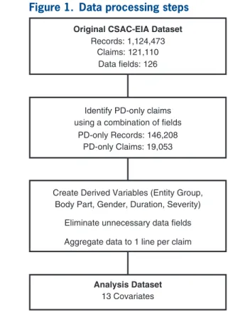
5. Data processing

In order to perform our survival analysis we pro-cessed the dataset to include only those variables that were necessary for our analysis, as well as creat-ing several derived variables. The data cleancreat-ing and mapping steps are illustrated in Figure 1.

In order to use the data for our PD survival analy-sis, it was first necessary to identify all PD claims (both permanent partial and permanent total) and their accompanying claim histories. Some claims were identified as temporary disability (TD) while they were undergoing initial evaluation and rating, potentially overstates claimant longevity as well as

the FM Reserves on PD claims. We tested the null hypothesis stating that termination rates in the claim-ant population are equal to the termination rates according to the current U.S. Life Table. Addition-ally, we developed a specific disabled termination table based on PD claimant data. While another table would be better than the U.S. Life Table if the null hypothesis is rejected, we demonstrate that the empirical termination table is better suited for the FM PD reserving calculation. Because our data includes a number of different variables, we have developed termination rates that depend on covari-ates, enabling the workers’ compensation claims adjuster to estimate duration to termination more accurately for a specific claimant.

4. Dataset description

Our dataset was provided by CSAC-EIA (the excess insurance carrier) which accumulates its data from third-party administrators of workers’ com-pensation claims as well as its own data. The data reflected detailed loss calculations for program years 1967/68 through 2015/16, evaluated annually from June 30, 1999 to June 30, 2016; there was little data prior to 1995. Although the data was provided by an excess insurer, all claims were recorded by the excess insurer are on a first dollar basis, whether or not the claim was a primary claim or an excess claim. While smaller entities may be more likely to seek excess insurance, we have no reason to suspect that this selection results in bias in terms of claimant termina-tions. The data included both indemnity and medical claim histories for all claim types (medical only, tem-porary partial, temtem-porary total, permanent partial, and permanent total).

Our initial data set consisted of 1,124,473 claim records for 121,110 unique claimants. Each data record corresponded to a different evaluation year of the claim, so that there were multiple records for each claimant depending on the date of the initial occur-rence, how many years the annual claim evaluations were performed by an adjuster and when the claim

Identify PD-only claims PD-only Claims: 19,053 using a combination of fields

PD-only Records: 146,208

Original CSAC-EIA Dataset

Records: 1,124,473 Claims: 121,110

Data fields: 126

Create Derived Variables (Entity Group, Body Part, Gender, Duration, Severity)

Analysis Dataset

13 Covariates

Eliminate unnecessary data fields Aggregate data to 1 line per claim

(5)

In addition, we created a new variable to indicate the severity of the injury or illness in terms of the likely cost of medical treatment. The new variable, labeled “Severity,” is the average annual claim amount paid during the duration of the claim. (Note that this defi-nition of Severity is specific to our analysis. Although similar, it is not the same as the traditional general insurance definition of severity.) We also created a new variable “Duration” which is the length of time from Date of Loss (DOL) to Date Closed.

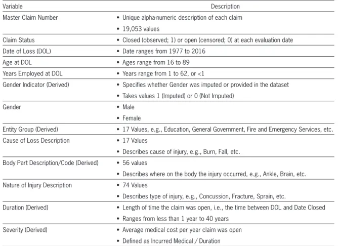
Next, we removed all variables that would not be used in our analysis in order to create our analysis dataset. This was done for ease of use as well as to improve the organization of our data. The variables in the analysis dataset are shown in Table 1.

Finally, multiple years of claims were merged into a single line per claim.

5.1. Data imputation for gender

The ‘Gender’ variable contained the values ‘Male,’ ‘Female’ and ‘Unknown/Other.’ We treated the ‘Unknown/Other’ values as missing. We consid-ered two options for handling missing data: delete the rows with missing gender values, or use imputation methods to predict the gender of the individual. We found that approximately 19% of the unique claims have the ‘Unknown/Other’ value for gender. Deleting the claims with missing gender values would signifi-cantly reduce our sample size. We therefore imputed the missing gender values using a logistic regression-based routine in R called MICE (Multivariate Imputation by Chained Equations) (For description of the routine and its application see, for example, Van Buuren and Groothuis-Oudshoorn (2011, 2017) and Analytics Vidhya (2016)). MICE uses observed values to fill in missing values on a variable-by- variable basis using logistic models for each variable and assuming that the gender values are MCAR (missing completely at random). It then takes our predictors and data with known gender values to find the most accurate model for imputing those with missing gender values through a parametric and stochastic search algorithm. The algorithm imputes and later changed to permanent disability after further

examination. A claim classified initially as TD and later re-classified as PD was re-classified as PD from inception. There was no single (reliable) variable indicating that a claim was a permanent disability. Therefore, we combined several variables from the original dataset (Claim Type, PD Incurred Flag, and Future Medical Award) to identify PD claims. This reduced the number of records from over 1.1 mil-lion in the original dataset to 146,208 records and 19,053 unique claims in our analysis dataset.

The quality of the data in the analysis dataset was generally good, aside from three variables: Entity Group, Body Part and Gender.

• Entity Group: Because of the large number of dif-ferent occupations we started with a higher level aggregation of occupations, labeled Entity Group, in order to reduce the dimensionality of the Occu-pation variable. However, the Entity Group data field provided with the original data was found to have many errors in terms of its mapping from the variable Occupation; over 50% of the occu-pations were coded as the ‘General Government’ occupation class. (For example the occupation ‘Police Officer’ was frequently coded as the ‘Gen-eral Government’ entity group, when it should correctly have been coded as ‘Police, Corrections, and Security’ entity group.) We created our own mapping using keywords found in various occu-pation descriptions to re-code the occuoccu-pations into 15 Entity Groups.

• Body Part: The original data file contained a numeric body part code to describe the body part(s) involved in the injury, but the field was poorly coded. The original data files had a Body Part description variable, a Nature of Injury vari-able, and a Cause of Loss variable which allowed us to re-map the body part descriptions to the appropriate body part code.

(6)

in which the event in question occurs at an unknown time after censoring. We also assume that censoring time is independent of survival time. Some important notation:

• Survival function: S(t) = P(T > t), which gives the probability of surviving beyond time t.

• Failure function: F(t) = 1 – P(T > t), which is the probability of failing before time t.

• Hazard function: h(t) = f (t)/S(t), which is the instantaneous rate of death at time t, given that the claimant is alive at time t.

• Cumulative hazard function: H(t) =∫t

0h(s)ds, which gives the cumulative rate of death up to time t, given that the claimant is alive at time t.

6.2. Kaplan-Meier estimator

Kaplan-Meier is a well-known method to estimate the survival function from given lifetime data. The incomplete values by generating ‘plausible’ synthetic

values given other columns in the data; each incom-plete column has its own specific set of predictors. The result of running the MICE algorithm is a derived Gender variable.

6. Methodology

6.1. Survival analysis

In many areas (such as biomedical, engineering, and social science), we are often interested in know-ing duration until an event occurs. Statistical analy-sis dealing with lifetime data is known as survival analysis. What makes these lifetime data sets unique and challenging to analyze is the presence of cen-sored information. Time until failure is not observed for all subjects during the study period, due to the fact that some subjects may be dropped out or lost to follow up. Our dataset contains right censored data,

Table 1. Analysis dataset summary

Variable Description

Master Claim Number • Unique alpha-numeric description of each claim • 19,053 values

Claim Status • Closed (observed; 1) or open (censored; 0) at each evaluation date

Date of Loss (DOL) • Date ranges from 1977 to 2016

Age at DOL • Ages range from 16 to 89

Years Employed at DOL • Years range from 1 to 62, or <1

Gender Indicator (Derived) • Specifies whether Gender was imputed or provided in the dataset • Takes values 1 (Imputed) or 0 (Not Imputed)

Gender • Male

• Female

Entity Group (Derived) • 17 Values, e.g., Education, General Government, Fire and Emergency Services, etc. Cause of Loss Description • 17 Values

• Describes cause of injury, e.g., Burn, Fall, etc. Body Part Description/Code (Derived) • 56 values

• Describes where on the body the injury occurred, e.g., Ankle, Brain, etc. Nature of Injury Description • 74 Values

• Describes type of injury, e.g., Concussion, Fracture, Sprain, etc.

Duration (Derived) • Length of time the claim was open, i.e., the time between DOL and Date Closed • Ranges from less than 1 year to 40 years

(7)

with coefficients  defined as r(X; ) = eβ′X_{. This} exponential form is convenient and flexible for many purposes allowing, among others, for the hazard function to have positive values (which is always the case by definition). Notice that no intercept term is included in β′X. Instead, it is subsumed in ho(t). The covariates are fixed at inception of the study and do not vary with time. Hazards are always positive. The model has two separate components: the baseline hazard function and the coefficients for covariates. Values of  can be estimated using the partial likeli-hood method (Kleinbaum and Klein 2012). However, the proportional hazards and functional form (linear combination of covariates) are strong assumptions which require careful examination (diagnostics). Extensions of Cox models, such as a time-dependent model or stratified Cox regression, can be applied in cases where the PH assumption is violated. The time-dependent model is beyond the scope of this paper. However, we consider a stratified Cox regression as one of our final models.

Assume covariates X₁, X₂, . . . , X_p satisfy the PH assumption while a covariate Z does not. The strati-fied Cox model is given by:

h t X

(

)

=h t eog( ) β′X

where g = 1, . . . , n are levels within covariate Z. Notice that the set of coefficients for each level is the same. The only difference is the shape of the base-line function for each level. The stratified Cox model allows the underlying baseline function to be varied across the levels by incorporating the covariate that violates the PH assumption into the baseline.

6.4. Model building and validation method

We created two different Cox models, one for imputed data and another for non-imputed data. In both cases, we randomly selected a training set consisting of 70% of observations with the remain-ing observations formremain-ing the validation set. The metric for model validation is the concordance index (c-index/c-statistic), which is a generalized version overall survival time is divided into small intervals

(t_i) by ordering the distinct failure times. Within each interval, the survival probability is calculated as the number of lives surviving over the num-ber of observed lives at risk. A simple estimate of Pr(T > t_i_T≥ t_i) is:

= − number of subjects surviving beyond t

number at risk at t

Y d

Y i

i

i i

i

An estimate of S(t) is ( )=

Π

 − 

  ≤

S t d

Y j t t

j

ˆ ₁ _where

Y_j is the number of subjects alive at time t_j and d_j is the number terminating at time t_j.

Subjects who have died, dropped out, or who have unobserved survival times are not at risk. Subjects that are considered as censored are counted in the denominator. Probability of surviving up to any point is estimated from the cumulative probability of surviving each of the preceding time intervals. A limitation of this method is that towards the end of the experiment, there are fewer observations, which makes the estimation less accurate than at the begin-ning of the study.

6.3. Cox proportional hazards model

Cox regression (proportional hazards or PH model) is an extension of regression techniques in survival analysis that allows us to examine the effect of multiple covariates on the hazard function. It is one of the most common models applied to survival data because of its flexible choice of covariates and ease of interpretation, as well as being fairly easy to fit using standard software. Let T be the continuous lifetime variable and X be a p × 1 vector of fixed covariates. The hazard function for T given X takes the form:

X X

(

)

= ( )

(



)

h t h t r0 ;

(8)

first array, denoted l_x, tracks the number of claims in the system at every age, with an initial count of 19,053 (the total number of claimants). The other two arrays, c_x and d_x respectively, count the number open (censored) and closed (observed) claimants at each age. With these arrays, it is possible to calculate estimates of qˆ_x, given that w_x = d_x + c_x, as defined above. qˆ_x is now an array of probabilities of claim closure for every age from 0 to 100. Finally we reduced the age range to 17 to 88 due to the lack of data outside of this range. The U.S. Life Table exists in both sex-specific and unisex forms. Below, we tested the consistency of our estimated qˆ_x with both the unisex table (Figure 2) and sex-distinct tables (Figure 3–4). It is clear that our estimated qˆ_x of area under the Receiver Operating Characteristic

curve (ROC curve). The concordance index is equiv-alent to rank correlation, where rank of predicted risk using the model for actual low risk observations (risk of experiencing the event) would be small while rank of predicted risk for high risk observa-tions would be large. Therefore C > 0.5 implies good predictive power, C = 0.5 implies predictive power is equivalent to 0, and C < 0.5 implies model does a poor job at prediction.

6.5. Actuarial methods

The 2011 Life Tables provide values of the one-year probability of death q_x from age x to x + 1. Workers compensation claims terminate for reasons other than death. The OSIP methodology requires the use of the mortality probabilities to estimate the future claim duration, so the q_x values represent all terminations, not just death. We estimate empirical

values of q_x from the data as

( )

= − ˆ

0.5

q d

l w

x x

where:

d_x= number of terminations between ages x and x+ 1.

l_x= number of claimants aged x C_n= number of censored claimants

w_x= number of claimants terminating during the year for any reason, including claims that are censored (denoted C_n), or still open at the end of the observation period.

In our model w_x= d_x+ c_x

In order to compare directly the modeling data-set to the 2011 U.S. Life Table we iterated through every claim and created vectors tracking the number of individuals in the system, the number that were censored (open) and the number observed (closed) at every age in the range 0 to 100, in order to match the 2011 Table’s range. To determine whether an individual was censored/observed and at which age, we used the indicator variable, the Age at DOL and the duration of each claim. By adding duration to the Age at DOL, it could be determined at what age every claim terminates, and by the indicator variable whether termination was censored or observed. The

Estimate q_x 95% Cl

Index

0 20 40 60 80 100

Qx

0.0

0.2

0.4

0.6

0.8

1.0

2011 life table q_x

Figure 2. Estimates of qx and comparison

with 2011 unisex life table (combined)

Index

0 20 40 60 80 100

QxF

0.0

0.2

0.4

0.6

0.8

1.0 Estimate q_x 95% Cl

2011 life table q_x

(9)

we do not have an assumption for the distribution of the samples. We assumed two samples are from the common distribution versus the alternative hypoth-esis that the CDF (cumulative density function) of the estimated qˆ_x is greater than the CDF of the 2011 life table. Because the p-value was less than the level of significance, we rejected the null hypothesis, confirming our conclusion that termination rates for both males and females are greater than the 2011 life table rates.

6.6. Fitted actuarial models

Given that the 2011 U.S. Life Table does not rep-resent termination rates of the workers’ compensation permanently disabled population, the question arises whether we can derive a better model for q_x?

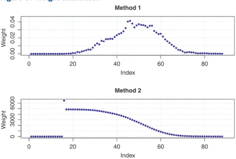
Note that all of the following regression models were tested assuming normal distribution errors and with two different types of weights included to repre-sent the number of obser vations in each age interval. The two methods to determine the weights were:

Method 1: The weight for each age interval is the proportion of the number of claims within the cor-responding interval to the total number of claims in the data.

Method 2: The weight for each age interval is the inverse of the length of each 95% confidence interval of the qˆ_x estimates.

We incorporated the weights into the regression models due to the observed pattern of heteroscedas-ticity (the constant variance in the errors is violated). Specifically, Method 2 allowed us to apply more weight to the observations with smaller standard errors as these observations carry more information in the data. In Figure 5 the two methods have differ-ent scales. The younger and older age intervals have relatively small weights in Method 1. For Method 2, early ages have higher weights, reflecting the lower variance at these ages, while higher ages are under-weighted, reflecting their higher variance.

We first fitted a quadratic function because this form appears to fit the observed qˆ_x values. The best values diverged from those of the 2011 Life Table,

thus implying that termination rates are higher in our data. In order to determine whether this divergence is significant, the 95% confidence interval for each age range was calculated by using Greenwood’s Approximation which estimates the variance of Kaplan Meier models, survival models equivalent to our qˆ_x values. In Greenwood’s Approximation,

(

)

s = q − q

d x

x x

x ˆ 1 ˆ 2

. 2

2

This approximation allowed us to calculate the 95% confidence interval for qˆ_x as qˆ_x ± 1.96 sx. In Figure 2, the lower bound of the confidence interval falls above the 2011 tabular rate at all ages except the highest (above age 85) at which there are very few observations.

In Figures 3 and 4 we examined the qˆ_x values for males and females separately. The results were similar to those of the unisex table, with the exception that some estimated qˆ_x values are less than the tabular values at very high ages at which there are very few observations. We concluded that in the age range 35–75 termination rates for both males and females are well in excess of the 2011 tabular rates. We also performed a one-sided Kolmogorov-Smirnov goodness-of-fit test to test whether the distribution between the 2011 life table and the estimated qˆ_x is identical. Specifically, we compared the empirical distribution function between two samples given that

Index

0 20 40 60 80 100

QxM

0.0

0.2

0.4

0.6

0.8

1.0 _{Estimate q_x}

95% Cl

2011 life table q_x

(10)

linear regression on the log transformation of the qˆ_x′s. The diagnostic plots of the log transformation for normality confirmed that we could proceed with the linear regression. To select the best Gompertz model, we first computed the lognormal log-likelihood for the log-transformed response, then calculated the AIC value. The resulting Gompertz model has the following form: qˆ_x = e–6.9188+0.0782x_{, using the set of} weights in Method 1.

The chosen Gompertz and quadratic models are shown in Figure 6, compared with the observed values fit quadratic model which included the set of weights

in Method 2 was qˆ_x= 0.0666 + 0.6289x + 0.2601x2_, which was selected via the AIC (Akaike Information Criterion) model selection method. AIC is found by computing 2k – 2lnLˆ, where Lˆ is the Maximum Likelihood function and k is the number of free parameters to be estimated.

Next we considered fitting the Gompertz model, which is one of the most commonly used parametric survival distributions to model human mortality. The Gompertz model assumes that the hazard rates are exponentially distributed where the hazard rates are analogous to the life table values q_x and are some parametric function of age (MacDonald, Richards, and Currie 2018). In the Gompertz model the hazard rate function, µx, generally has the following form: µ_x = eα+βx, where x denotes age of individual, and

µx and qx are related as follows: qx=∫ 1

0 spxµx+sds. In this formula, the two parameters represent an age-dependent (β) and age-independent component (α). The log transformation of this hazard rate func-tion is a linear funcfunc-tion α + βx. We estimated the parameters of the Gompertz model by performing

0 20 40 60 80

0 20 40 Index

0.00

0.02

0.04

W

eight

03

00

06

00

0

We

ight

Index

60 80

Method 1

Method 2

Figure 5. Weight distribution

Table 2. AIC values of fitted models using different weights

AIC value Method 1 Method 2

Quadratic Model −403.0 −465.1

Gompertz Model −296.9 −209.1 0 20 _time

Quadratic Gompertz

40 60 80

Qx

0.00

0.05

0.10

0.15

0.20

0.25

(11)

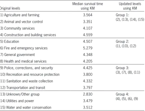
level costs a degree of freedom to estimate, whereas a majority of these levels are not significant. We therefore required a method to simplify the multi-level variables to a smaller number of groups. We applied the Kaplan Meier (KM) approach to re-group levels based on median survival time. We first applied KM to estimate the survival function to obtain median survival time. Second, we ranked median survival times in increasing order and re-grouped the original levels into four different groups. We then repeated this procedure for Entity, Cause of Loss, and Body Parts. Table 3 shows the new grouping of the Entity variable. (See Appendix A2 for groupings of the Cause of Loss and Body Parts variables).

The new grouping is based on the application of the KM method to the training set; we then applied the same groupings to the test set.

7.2. Stratified Cox model

The final model contains two interaction terms: interaction between Sex and Age at DOL, and between Body Parts and Cause of Loss. The Entity Group covariate did not satisfy the PH assumption, and we therefore created stratified Cox models for the differ-ent levels of Entity.

for q_x. The age range on the x-axis is determined empirically based on available data (ages 16 to 88). The y-axis contains the qˆ_x estimates, or the prob-ability of claim closure for a given age, x. Both the Gompertz and quadratic models fit the data reason-ably well up to age 60, although, as shown in Table 2, the quadratic model fits better (lower AIC value). Thereafter, the Gompertz model significantly over-estimates termination, as does the quadratic model above age 70.

7. The Cox model applied

to imputed data

7.1. New grouping of entity,

cause of loss, and body parts

Several covariates such as Entity Groups, Cause of Loss, and Body Parts are categorical with many levels. For example, the Body Parts variable contains 56 values that indicate the location of the injury. While the translation of the Body Part description into numeric values is convenient for coding pur-poses, Body Part is a nominal variable where levels do not have any natural order. A drawback of fitting Cox regression is model complexity: each covariate

Table 3. Grouping of entity variable

Original levels Median survival time using KM Updated levels using KM

(1) Agriculture and farming 3.564 Group 1:

(2), (13), (14), (15)

(2) Animal and vector control 3.351

(3) Community services 4.107

(4) Construction and building services 4.559

(5) Education 4.507 Group 2:

(1), (10), (12)

(6) Fire and emergency services 5.279

(7) General government 4.348

(8) Health and medical services 4.205

(9) Police, corrections, and security 4.425 Group 3:

(3), (7), (8), (11) (10) Recreation and resource protection 3.800

(11) Sanitation and waste collection 4.332

(12) Transportation and transit 3.797

(13) Unknown/Other group 2.830 Group 4:

(4), (5), (6), (9)

(14) Utilities and power 3.479

(12)

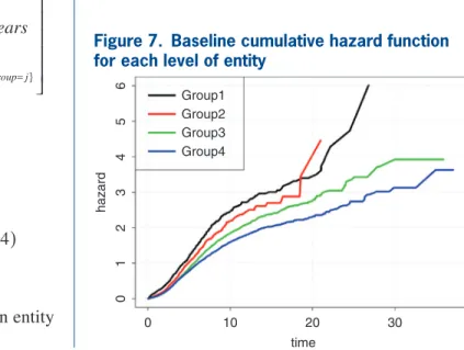
Figure 7 shows the shapes of the baseline hazard functions for each entity group. The shapes of the cumulative baseline hazard functions for the entity levels are not always parallel; in particular the group 2 function crosses group 1, violating the PH assump-tion. Three different tests, the likelihood ratio test, Wald’s test, and log-rank test are conducted to test The functional form of the stratified Cox model is

h t X h t

age

severity sex

years sex years og

j body j j

j CL group j j

j body j CL group j j

∑

(

)

= ( )

β + τ

+ γ

+ β + β

+ δ                           { } { } { } { } = = = = = = = I I I I ˆ _exp ˆ _ˆ ˆ ˆ ˆ

ˆ ˆ _:

ˆ 1 ₂ 4 2 4 3 4 5 6 2 4

cause loss group j j

otherwise

CL group j = =

(

=

)

     { =} I where 1,

2, 3, 4

0,

body j j

otherwise body j

(

)

=_ = =  { =}

I 1, 2, 3, 4

0,

g= 1, 2, 3, and 4 levels within entity

group. time

hazard

0

012345

6

10 20 30 Group4

Group3 Group2 Group1

Figure 7. Baseline cumulative hazard function for each level of entity

Table 4. Stratified Cox model on imputed data

Covariates Coeff. Hazard ratio Std. error P-value 95% CI of HR

Age at DOL −0.007 0.993 0.01 0.000 0.990, 0.996

Body 2 (vs. 1) −0.125 0.882 0.190 0.510 0.608, 1.281

Body 3 (vs. 1) −0.572 0.565 0.191 0.003 0.389, 0.820

Body 4 (vs. 1) −0.605 0.546 0.245 0.014 0.338, 0.883

Cause loss 2 (vs. 1) 0.040 1.041 0.147 0.786 0.781, 1.388

Cause loss 3 (vs. 1) −0.420 0.657 0.362 0.247 0.323, 1.337

Cause loss 4 (vs. 1) −0.231 0.794 0.149 0.121 0.593, 1.063

Severity 0.000 1.000 0.000 0.000 1.000, 1.000

Sex −0.542 0.581 0.098 0.000 0.480, 0.704

Years employed −0.008 0.992 0.001 0.000 0.989, 0.995

Age at DOL: Sex 0.010 1.010 0.002 0.000 1.006, 1.015

Body 2: Cause loss 2 −0.308 0.735 0.199 0.123 0.498, 1.087

Body 3: Cause loss 2 −0.087 0.917 0.197 0.658 0.623, 1.348

Body 4: Cause loss 2 −0.325 0.723 0.251 0.195 0.442, 1.181

Body 2: Cause loss 3 0.352 1.422 0.423 0.405 0.621, 3.256

Body 3: Cause loss 3 0.528 1.695 0.402 0.189 0.771, 3.730

Body 4: Cause loss 3 0.234 1.264 0.435 0.590 0.539, 2.962

Body 2: Cause loss 4 −0.079 0.924 0.197 0.689 0.628, 1.360

Body 3: Cause loss 4 0.111 1.117 0.197 0.573 0.760, 1.642

(13)

(a) Overall fit

Cox-Snell residuals, defined as r_i= Hˆ₀(T_i)eβˆXi, can be

used to assess the overall fit of our Cox Proportional Hazards model. If the model is correct, a plot of the residuals of the estimated cumulative hazard rates Hˆ₀(r_i) versus r_i should follow a straight line through the origin. In Figure 8, we see the estimated cumula-tive hazard is close to the diagonal line for all but large values of Cox-Snell residuals.

Overall, the model fits the data well as the pro-portion of the observations in the early range [0,4] of Cox-Snell residuals is approximately 99.8% of the whole training set. The departure of the estimated cumulative hazard as Cox-Snell residuals get larger indicates the presence of the potential outliers in the data.

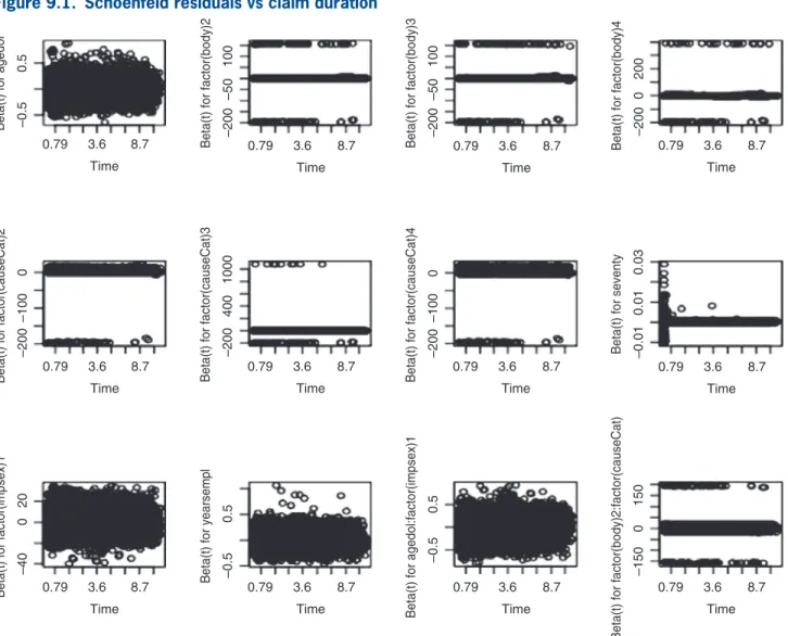
(b) Appropriateness of the proportional hazard assumption

The departure from proportionality could lead to an incorrect model. We examined the PH assumption in two ways: by plotting the Schoenfeld residuals and performing a formal hypothesis test for correlation between Schoenfeld residuals and time.

If the PH assumption is true, we should expect that the trend of β(t) versus time to be a horizontal line the global hypothesis that  =0 (overall

goodness-of-fit). As p-values for all three tests are close to 0, we reject the null hypothesis, indicating that the model is an appropriate fit for the data set.

7.3. Model interpretation

Coefficients of the Cox model are related to the hazard rate. For example, the coefficient value of −0.008 for Years Employed at DOL indicates that the log hazard ratio increases by a unit of −0.008 for each additional unit increase in years of employ-ment while other variables are kept constant. In practice, it is more meaningful to interpret the result using hazard ratio (or relative risk) instead of log hazard ratio.

The hazard ratio is obtained by taking the expo-nential of the coefficient. Specifically, the hazard ratio of years employed is e(−0.008)=_{0.992, indicating} that for each additional unit increase in duration of employment while holding other variables constant, the hazard ratio increases by a factor of 0.992. In other words, the risk of claim termination decreases by about 1% for each yearly increase in number of years employed.

The final model contained two significant inter-action terms: interinter-action between Sex and Age at DOL (categorical vs. continuous) and interaction between Body Parts and Cause of Loss (two categorical vari-ables). When interaction terms are significant, the interpretation of the coefficients becomes much more complex. For example, interpretation of “Sex and Age at DOL” is not as simple as Years Employed. The significant interaction between Sex and Age at DOL implies that the effect of DOL on the sur-vival rate varies for each sex (male and female). Specifically, for each unit increase in age at DOL for a male claim, the hazard ratio increases by a factor of 1.010.

7.4. Model diagnostics

We tested the validity of the assumptions made in

the model with model diagnostics. Cox-Snell residuals

Cumulative hazard

0

01234567

2 4 6 8 10

(14)

(c) Linear form of covariates

We further examined whether the linear combination of covariates is the best functional form to describe the effect of the covariates on survival. To do this, we plotted the martingale residuals versus each covariate. The results in Figure 10 implied that we did not need any polynomials or transformation of the covariates.

(d) Outliers and influential points

We examined the accuracy of the model for predicting the survival of a given subject. In other words, we tried to find claims whose survival time differed significantly in comparison to their model predictions. The deviance residuals plot versus risk for each covariate. As we see in Figures 9.1 and 9.2,

the pattern of each plot looks horizontal around zero with little violation, implying that the PH assumption is valid.

To examine PH assumption more carefully, we performed a hypothesis test which Grambsch and Therneau (1994) proposed. Each parameter in the model is allowed to depend on time (i.e., βj(t) = βi +γjgj(t)). We tested the value of the correlation parameter γj; if γj= 0 we would reject the hypothesis that parameters are time-dependent. We conducted this test using function cox.zph in R and observed that all p-values are not significant (Table 5). In summary, we did not have sufficient evidence to reject the null hypothesis that the PH assumption is valid.

Beta(t) for agedol –0.5

0.5

Beta(t) for factor(body)2 –200

100

–50

Beta(t) for factor(causeCat)3

–200

1000

400

–200

0

–100

Beta(t) for factor(impsex)1

–40

20

0

Beta(t) for factor(body)2:factor(causeCat

)

–150

150

0

Beta(t) for yearsempl –0.5

0.5

Beta(t) for agedol:factor(impsex)1

–0.5

0.5

100

–50

–200

0

–100

200

0

Beta(t) for seventy _–0.01

0.03

0.01

0.79 3.6 Time

8.7

0.79 3.6 Time

8.7

0.79 3.6 Time

8.7

0.79 3.6 Time

8.7

0.79 3.6 Time

8.7

0.79 3.6 Time

8.7

0.79 3.6 Time

8.7

0.79 3.6 Time

8.7

0.79 3.6 Time

8.7

0.79 3.6 Time

8.7

0.79 3.6 Time

8.7

0.79 3.6 Time

8.7

(15)

Beta(t) for factor(body)3:factor(causeCat)2

–50

–150

150

05

0

–200

–400

100

0

–600

–200

–1000

200

–600

–200

–1000

200

0

Beta(t) for factor(body)4:factor(causeCat)

3

–600

–20

0

–1000

200

0

4

–50

–15

01

50

0

4

–50

–15

01

50

0

4

–20

0

–40

01

00

0

0.79 3.6 Time

8.7 0.79 3.6 Time

8.7

0.79 3.6 Time

8.7 0.79 3.6 Time

8.7

Figure 9.2. Schoenfeld residuals vs. claim duration (cont’d)

Table 5. PH Assumption hypothesis test results

Covariates hypothesis testp-value for Covariates hypothesis testp-value for

Age at DOL 0.662 Age at DOL:Sex 0.841

Body 2 0.824 Body 2: Cause of loss 2 0.751

Cause of loss 2 0.634 Body 2: Cause of loss 3 0.929

Severity 0.343 Body 2: Cause of loss 4 0.834

Sex 0.651 Body 3: Cause of loss 4 0.614

(16)

and x is the matrix of value of covariates. We per-formed further sensitivity analysis by removing these out liers and refitting the model. The new fitted model is not far off from the model presented in Table 3, and pre dictive power for both models using c-index is similar.

We also examined the influence of each claim on the model fit. The scaled score statistics versus covariate plot allows us to find influence points. Figure 12.1 and 12.2 show score residuals for each covariate. Using the plot between severity and the scaled score statistics, we observed several points that were further away from the majority of the observations, although this distance does not appear to be significant, suggesting that these points may be exercising influence on the fit.

7.5. Model prediction

We applied the final Cox model to the test set and calculated the concordance index. A C-index scores is helpful to detect which claims are potential

outliers, which perhaps should be excluded from the analysis. In Figure 11, we observe that the deviance residuals are randomly scattered in the panel and some observations (marked as triangles with indices) are the detected potential outliers. “Risk Score” is defined as

Σ

βx, where β is the vector of coefficients

–1

0–

8–

6–

4–

20

Martingale Residuals

–1

0–

8–

6–

4–

20

–1

0–

8–

6–

4–

20

–1

0–

8–

6–

4–

20

–10

–8

–6

–4

–2

0

–10

–8

–6

–4

–2

0

–10

–8

–6

–4

–2

0

–10

–8

–6

–4

–2

0

20 40 60 80 1.0 2.0 3.0 4.0 1.0 2.0 3.0 4.0 0 5000 15000

agedol

20

0 40 60 80

sex:agedol 20

0 40 60

0.4

0.0 0.8

years employment sex

5 10 15

cause:body cause

body part severity

Figure 10. Martingale residuals vs. covariate

0 2 4 6

–2

Risk Score

De

viance Residuals

–4

–2

024

11430

11511 2577 7799

431

10648

12782 3578

960 6821 3570 4181

(17)

8.1. Discussion

Workers’ compensation reserves for future medi-cal liabilities are usually medi-calculated in bulk using a triangle method. Although this standard method is widely used, there are examples of studies using reserving methods based on mortality projections, recognizing that explicit incorporation of injured worker mortality may reduce the potential inaccuracy in the bulk reserves. The State of California requires an explicit calculation for each permanently injured worker, assuming that termination of the claim fol-lows the most recent U.S. Life Table. The literature shows that injured worker mortality is higher than that of the overall population, which could lead to over-reserving of future medical liabilities. We examined claims termination rates of injured workers of 0.58 indicates the model does a moderately

good job at predicting the risk of the claim being terminated.

8. Results of Cox model

on non-imputed data

We will not repeat specific details for this section as all the procedures are similar to imputed data. Table 6 presents the final form of the Cox model on the non-imputed data. It contains three interaction terms: between Sex and Age at DOL, between Entity Group and Sex, and between Body Parts and Cause of Loss. When applied to the test dataset, the C-index of 0.57 indicates that model does a good job at pre-dicting the risk of the claim being terminated.

Scaled Score Residuals Scaled Score Residuals Scaled Score Residuals Scaled Score Residuals

–0.1

0.

00

.1

0.

2

–0.2

0.

00

.2

0.

4

–0.2

0.

00

.2

0.

4

–0.3

–0.1

0.

10

.3

–0.

10

.1

0.

30

.5

–0.10

0.00

0.10

0.20

–0.10

–0.05

0.00

0.05

–0.20

–0.10

0.00

0.10

–0.4

–0.

20

.0

0.

2

–0.

10

.1

0.

30

.5

–2.

5

–1.5

–0.5

–0.

8

–0.

40

.0

0.

3

agedol factor(body)2 factor(body)3 factor(body)4

factor(causeCat)2 factor(causeCat)3 factor(causeCat)4 severity

20 40 60 80

20

0 40 60 80

10

0 30 50

0.0 0.4 0.8

0 5000 15000

0.0 0.4 0.8 0.0 0.4 0.8

0.0 0.4 0.8

0.0 0.4 0.8 0.0 0.4 0.8

factor(impsex)1 yearsempl agedol:factor(impsex)1 factor(body)2:factor(causeCat)2

(18)

0.79 3.6 8.7

0.79 3.6 8.7 0.79 3.6 8.7 0.79 3.6 8.7 0.79 3.6 8.7 0.79 3.6 8.7 0.79 3.6 8.7 0.79 3.6 8.7

–150

–50

50

150

0

–150

–50

50

150

0

–400

–200

100

0

–400

–200

100

0

–1000

–600

200

–200

–1000

–600

200

–200

0

–1000

–600

200

–200

0

–150

–50

50

150

0

Beta(t) f

or f

actor(body)3:f

actor(causeCat)2

Beta(t) f

or f

actor(body)4:f

actor(causeCat)2

Beta(t) f

or f

actor(body)2:f

actor(causeCat)3

Beta(t) f

or f

actor(body)3:f

actor(causeCat)3

Beta(t) f

or f

actor(body)4:f

actor(causeCat)3

Beta(t) f

or f

actor(body)2:f

actor(causeCat)4

Beta(t) f

or f

actor(body)3:f

actor(causeCat)4

Beta(t) f

or f

actor(body)4:f

actor(causeCat)4

Time Time Time Time Time Time Time Time

Figure 12.2. Scaled residuals vs. covariate (cont’d)

Table 6. Final Cox model on non-imputed data

Covariates Coeff. HR Std. errors P-value 95% CI of HR

Entity 2 −0.206 0.814 0.123 0.094 0.6400, 1.0358

Entity 3 −0.526 0.591 0.104 0.000 0.4817, 0.7253

Entity 4 −0.600 0.549 0.107 0.000 0.4451, 0.6772

Age at DOL 0.003 1.003 0.002 0.062 0.9998, 1.0069

Body 2 −0.581 0.560 0.140 0.000 0.4255, 0.7359

Body 3 −0.603 0.547 0.207 0.004 0.3649, 0.8204

Body 4 −0.874 0.417 0.165 0.000 0.3020, 0.5766

Cause loss 2 −0.610 0.543 0.165 0.000 0.3931, 0.7506

Cause loss 3 −0.461 0.630 0.119 0.000 0.4992, 0.7961

Cause loss 4 −0.282 0.754 0.102 0.006 0.6173, 0.9216

Severity 0.000 1.000 0.000 0.000 1.0002, 1.0002

Sex male 0.291 1.337 0.163 0.075 0.9711, 1.8421

Years employment −0.006 0.994 0.001 0.000 0.9913, 0.9971

(19)

using the experience of the California Association of Counties-Excess Insurance Authority (CSAC-EIA). We applied a number of different methods, includ-ing direct calculation of the termination rates (qˆ_x) (both raw and fitted to polynomials) to compare with the tabular rates, and found that for most ages, termi-nation rates are in excess of

those implied by the tabular rates. Finally, we applied Cox Proportional Hazards model-ing to develop termination hazard rates based on our dataset. The Cox PH model is powerful in that it allows us to incorporate covariates and to assess the influence of individual covariates on the termination hazard. Tests of the proportional hazard assumptions show that the Cox model fits the data well, and that we can have confi-dence in the derived model.

8.2. Conclusion

Analysis of the CSAC-EIA data shows that the use of the standard population mortality

table as the basis for permanent disability claim projections may be inappropriate because the table overestimates injured worker survival. However, it is important to remember that the life expectancy of the injured worker is only one component of the reserve calculation; the other component is the

aver-age 3-year cost of medical claims. Because the claims cost component excludes a provision for medical trend, it may underestimate the future medical cost component. The result of combining an over-estimate of survival with an underestimate of future med-ical costs may well result in reasonable reserves in total; however, if the intention is to produce accurate reserves for future medical claims, more accurate methods of estimating both life expec-tancy and future medical claims would be appropriate.

8.3. Limitations

This study was performed on the experience of one

We applied Cox Proportional

Hazards modeling to develop

termination hazard rates based

on our dataset. The Cox PH model

is powerful because it allows us

to incorporate covariates and to

assess the influence of individual

covariates on the termination

hazard. Tests of the proportional

hazard assumptions show that

the Cox model fits the data well,

and that we can have confidence

in the derived model. The effect

of covariates on the hazard rates

provides more information to

claims managers about the likely

survival of specific claimants than

the standard table.

Entity 2: Sex male 0.280 1.324 0.155 0.070 0.9777, 1.7918

Entity 3: Sex male 0.416 1.515 0.130 0.001 1.1750, 1.9537

Entity 4: Sex male 0.298 1.348 0.132 0.023 1.0412, 1.7444

Body 2: Cause loss 2 0.672 1.958 0.216 0.002 1.2825, 2.9902

Body 3: Cause loss 2 0.539 1.714 0.299 0.071 0.9543, 3.0787

Body 4: Cause loss 2 0.417 1.517 0.243 0.087 0.9413, 2.4440

Body 2: Cause loss 3 0.401 1.493 0.162 0.013 1.0875, 2.0489

Body 3: Cause loss 3 0.255 1.291 0.226 0.259 0.8284, 2.0120

Body 4: Cause loss 3 0.394 1.482 0.183 0.032 1.0354, 2.1223

Body 2: Cause loss 4 0.247 1.281 0.145 0.088 0.9637, 1.7020

Body 3: Cause loss 4 0.058 1.060 0.212 0.784 0.6997, 1.6054

Body 4: Cause loss 5 0.117 1.125 0.170 0.490 0.8062, 1.5685

Table 6. Final Cox model on non-imputed data (cont'd)

(20)

in Taiwan. Accident Analysis and Prevention 38, 2006, pp. 961–968.

Jones, B. A., C. J. Scukas, K. S. Frerman, M. S. Holt, and V. A. Fendley, “A Mortality-Based Approach to Reserving for Lifetime Workers’ Compensation Claims,” CAS E-Forum, Fall 2013, pp. 1–26.

Kleinbaum, D. G., and M. Klein, Survival Analysis, 3rd ed., New York: Springer Verlag, 2012.

Lin, S.-H., H.Y. Lee, Y.-Y. Chang, Y. Jang, and J.-D. Wang, “Estimation of Life Expectancies and Loss-of-Life for Workers with Permanent Occupational Disabilities,” Scandina-vian Journal of Work Enviroment Health 38, 2012, pp. 70–77. Liss, G. M., S. M. Tarlo, D. Banks, K.-S. Yeung, and

M. Schweigert, “Preliminary Report of Mortality Among Workers Compensated for Work-Related Asthma,” American Journal of Industrial Medicine 35, 1999, pp. 465–71. MacDonald, A. S., S. J. Richards, and I. D. Currie, Modeling

Mortality and Longevity with Actuarial Applications, London: Cambridge University Press, 2018.

Schmid, F. A., “The Workers Compensation Tails,” Variance 6, 2012, pp. 48–79.

Sears, J. M., L. Blanar, and M. Bowman, “Predicting Work-Related Disability and Medical Cost Outcomes: A Comparison of Injury Severity Scoring Methods,” Injury: International Journal of the Care of the Injured 45, 2014, pp. 16–22. Sears, J. M., L. Blanar, S. M. Bowman, D. Adams, and B. A.

Silverstein, “Predicting Work-Related Disability and Medi-cal Cost Outcomes: Estimating Injury Severity Scores from Workers’ Compensation Data,” Journal of Occupational Rehabilitation 23, 2013, pp. 19–31.

Shane, M. and D. Morelli, “Using Life Expectancy to Inform the Estimate of Tail Factors for Workers Compensation Liabilities,” CAS E-Forum, 2013.

Sherman, R., and G. F. Diss, “Estimating the Workers’ Compen-sation Tail,” Proceedings of the Casualty Actuarial Society, 2006.

State of California, Estimating and Reporting Work Injury Claims., Dept. of Industrial Relations, 2011, Sacramento, CA.

van Buuren, S., and K. Groothuis-Oudshoorn, “mice: Multivariate Imputation by Chained Equations in R,” Journal of Statistical Software 45, 2011, p. 63.

van Buuren, S., and K. Groothuis-Oudshoorn, Package ‘mice’, 2017, cran-R.org.

Wedegaertner, F., S. Arnhold-Kerri, N.-A. Sittaro, S. Bleich, S. Geyer and W. E. Lee, “Depression- and Anxiety-Related Sick Leave and the Risk of Permanent Disability and Mortal-ity in the Working Population in Germany: A Cohort Study,” BMC Public Health 13(145), 2013, pp. 1–10

pool, incorporating a number of different third-party administrators. Changes in reporting requirements and administrators over time may affect the accu-racy of the data. As noted in our conclusion, life expectancy is only one component of the reserving calculation, and reserves calculated according to the State of California methodology may be appropri-ate because different components of the calculation offset each other.

Acknowledgments

The authors acknowledge with gratitude the collaboration of CSAC-EIA and its chief actuary, John Alltop FCAS MAAA, in the preparation of this study, as well as UCSB students Shannon Nicponski, MS; Elizabeth Riedell, BS; and Jerrick Zhang, BS, who performed the initial analysis. This work was supported in part by a CAE 2016 grant from the Society of Actuaries.

References

Analytics Vidhya, “Tutorial on 5 Powerful R Packages Used for Imputing Missing Values,” Analytics Vidhya, 2016, https:// www.analyticsvidhya.com/blog/2016/03/tutorial-powerful- packages-imputing-missing-values/.

Arias, E., ed., United States Life Tables, 2011, Division of Vital Statistics, 2015, p. 63.

CAS (Casualty Actuarial Society) Tail Factor Working Party, “The Estimation of Loss Development Tail Factors: A Summary Report,” Arlington, VA: Casualty Actuarial Society, 2013. Dickson, D. C. M., M. R. Hardy, and H. R. Waters, Actuarial

Mathematics for Life Contingent Risks, 2nd ed., New York: Cambridge University Press, 2013.

Gillam, W. R., “Injured Worker Mortality,” Proceedings of the Casualty Actuarial Society 80, 1993, pp. 34–54.

Grambsch, P., and T. M. Therneau, “Proportional Hazards Tests and Diagnostics Based on Weighted Residuals,” Biometrika 81, 1994, pp. 515–26.

(21)

Appendix. Data Summary

Table A.1. Original variables

Variable Description

Original Excel # • The row number in original dataset (1,124,473 rows total)

Gender • Female

• Male

• Unknown/Blank

Master Claim Number • Unique alpha-numeric description of each claim • 121,110 values

Claim Type • Dupe/Delete

• First Aid • Future Medical • Indemnity • Info Only • Medical Only • Other

• Temporary Disability

Date of Loss (DOL) • Dates range from 1967 to 2016

• 3.5% of records relate to accident years 1994 & prior

Age at DOL • Ages range from 1 to 97

• Missing Values (fewer than 2%) Claim Status at 6–30–2016 • Open

• Closed

• ReOpened-Closed • Blank

Occupation • 2,624 occupational descriptions

• e.g. Firefighter, Teacher, Accountant, Electrician

Entity Group • 17 Departments e.g. Education, General Government, Fire and Emergency Services, etc.

Date Closed • Date ranges from 8/1/77 to 6/30/2016

Average Weekly Wages • Ranges from $0.00 to $33,446.40 • Missing Values (over 50% of data)

Nature of Injury Description/Code • 74 values, e.g. Sprain, Fracture, Hearing Loss, Concussion, etc.

Future Medical Award • TRUE or FALSE

PD Incurred Flag • TRUE or FALSE

Incurred Medical • Incurred Medical = Total dollar amounts of medical payments paid plus reserves for future medical costs Incurred PD • Numeric values ranging from $0.30 to $1.8 million

• Incurred PD = Paid PD + Reserved PD

• Refers to indemnity benefits (paid to worker to compensate for lost wages) on PD claims, not medical benefits

Years Employed at DOL • Years range from 1 to 62, or <1 • Missing values (approx 4.5%)

(22)

Table A.2. New grouping of cause of loss in imputed data

Original level Median survival time using KM New grouping

(1) CL1: Absorption, ingestion, or inhalation 4.211 Group 1:

(5), (12), (14), (15)

(2) CL2: Animal or insect 4.893

(3) CL3: Burn 4.192

(4) CL4: Caught 3.493

(5) CL5: Cut 3.455 Group 2:

(4), (8), (10), (11)

(6) CL6: Explosion or flare back 5.178

(7) CL7: Fall 4.274

(8) CL8: Fellow worker, patient, or other person 3.597

(9) CL9: Machine or tool 4.181 Group 3:

(1), (3), (9)

(10) CL10: Miscellaneous 4.090

(11) CL11: Motor vehicle 3.978

(12) CL12: Natural disasters 1.268

(13) CL13: Person in act of a crime 4.274 Group 4:

(2), (6), (7), (13), (16), (17)

(14) CL14: Rubbed 2.745

(15) CL15: Slipped 3.332

(16) CL16: Strain 4.474

(17) CL17: Strike 4.356

Table A.3. New grouping of body parts in imputed data

Original level

(description with numeric code) Median survival time using KM New grouping

(1) other −9 3.074 Group 1:

(9), (12), (14), (16), (24), (36), (37), (52), (54), (58), (62), (64), (66), (99).

(2) multiple head injury −10 5.063

(3) skull −11 3.816

(4) brain −12 2.773

(5) ear(s) −13 5.132

(6) eye(s) −14 2.964

(7) nose −15 5.267

(8) teeth −16 1.996

(9) mouth −17 3.830

(10) other facial soft tissue -18 5.405

(11) facial bones −19 9.266

(12) multiple neck injury −20 4.668

(13) vertebrae −21 4.600

(23)

(15) spinal cord −23 4.429 Group 2:

(11), (17), (31), (32), (33), (35), (38), (39), (44), (46), (55), (56), (61), (65), (11), (17), (31), (32), (33), (35), (38), (39), (44), (46), (55), (56), (61), (65).

(16) larynx −24 1.956

(17) soft tissue neck −25 5.044

(18) multiple upper extremities −30 4.375

(19) upper arm incl. clavicle and scapula −31 3.644

(20) elbow −32 3.438

(21) lower arm −33 3.658

(22) wrist −34 4.274

(23) hand −35 4.060

(24) finger(s) −36 2.803

(25) thumb −37 3.096

(26) shoulder(s) −38 3.929

(27) wrist(s) and hand(s) −39 4.195

(28) multiple trunk −40 4.532

(29) upper back area −41 5.219 Group 3:

(20), (21), (23), (30), (34), (40), (42), (45), (48), (50), (51), (53), (57), (91).

(30) lower back area −42 4.877

(31) disc trunk −43 5.266

(32) chest −44 3.534

(33) sacrum and coccyx −45 4.359

(34) pelvis −46 3.868

(35) spinal cord −47 6.888

(36) internal organs −48 4.753

(37) heart −49 8.932

(38) multiple lower extremities -50 4.348

(39) hip −51 4.932

(40) upper hip −52 3.066

(41) knee −53 4.249

(42) lower hip −54 2.921

(43) ankle −55 3.501 Group 4:

(10), (13), (15), (18), (19), (22), (25), (41), (43), (47), (49), (60), (63), (90).

(44) foot −56 3.674

(45) toe(s) −57 4.258

(46) great toe −58 1.508

(47) lung −60 5.501

(48) abdomen incl. groin -61 3.321

(49) buttocks −62 2.992

(50) lumbar and/or sacral vertebrae −63 5.638 (51) artificial appliances (braces, etc.) −64 2.452 (52) insufficient info to identify/unclass −65 4.085

(53) no physical injury −66 2.721

(54) multiple body parts −90 5.227

(55) body system and mult. body systems −91 4.611

(56) whole body −99 2.978

Table A.3. New Grouping of Body Parts in Imputed Data (cont'd)

Original level