Sharif University of Technology
Scientia IranicaTransactions A: Civil Engineering www.scientiairanica.com
Adaptive mesh-free lower bound limit analysis using
non-linear programming
S.M. Binesh
and S. Rasekh
Department of Civil and Environmental Engineering, Shiraz University of Technology, Shiraz, Iran. Received 23 December 2015; received in revised form 7 June 2016; accepted 19 July 2016
KEYWORDS Adaptive; Mesh-free; Lower bound; Non-linear programming; Plane strain.
Abstract.An adaptive mesh-free approach is developed to compute the lower bounds of limit loads in plane strain soil mechanics problems. There is no pre-dened connectivity between nodes in the mesh-free techniques, and this property facilitates the implementation of h-adaptivity. Nodes may be added, moved, or discarded without complex changes in the data structures involved. In this regard, the Shepard mesh-free method is used in conjunction with the nodal stress rate smoothing technique and the lower bound limit analysis theory to establish a non-linear optimization problem. This problem is solved by the second-order cone programming technique, and the result is a stress eld that satises the lower bound requirements in a non-rigorous manner. The lack of rigorousness arises from relaxation during nodal stress rate smoothing process. An error estimator is introduced by the application of Taylor series expansion, and by controlling the local error via a user-dened tolerance, the adaptive renement strategy is established. To demonstrate the eectiveness of the proposed method, the procedure is applied to the examples of purely cohesive and cohesive-frictional soils.
© 2017 Sharif University of Technology. All rights reserved.
1. Introduction
Limit theorems of classical plasticity [1] can be very powerful for estimating collapse loads of geo-structures. However, their applications by hand are restricted to simple problems where it is possible to assume obvious failure mechanisms or stress discontinuities. Therefore, much progress has been made over the last three decades on the development of numerical limit analysis techniques using the combination of nite-element method and limit theorems. These methods, known as nite-element limit analyses, are very general and can
*. Corresponding author.
E-mail addresses: [email protected] (S.M. Binesh); rasekh.sara72@yahoocom (S. Rasekh)
doi: 10.24200/sci.2017.4163
deal with complex practical problems, where the failure load is dicult to estimate by the other methods. A complete review on the development of dierent nite-element limit analysis techniques for geotechnical stability analysis was provided by Sloan [2].
In the nite-element limit analysis, the discretiza-tion of domain is carried out by the nite-element method. However, in some recent studies, the mesh-free methods have been used as the discretization tool with the goal of computational eciency improvement. For example, Chen et al. [3] developed a lower bound approach using the element-free Galerkin method and reduced-basis technique to construct an admissible stress eld. Chen et al. [4] also applied the element-free Galerkin method to the lower bound shakedown anal-ysis of structures under variable repeating loads. Le et al. [5,6] used element-free Galerkin method to discretize the moment eld in the limit analysis of plates. Liu and
Zhao [7] used the radial point interpolation method and nonlinear programming to develop a technique for upper bound limit analysis of solid structures. Binesh and Raei [8] combined the theory of limit analysis with the stabilized nodal integration scheme and the radial point interpolation method to provide an approach for estimating the upper bound of the limit loads in purely cohesive soils. Binesh and Gholampour [9] introduced a mesh-free lower bound limit analysis approach by the application of the Shepard's shape functions and the linear programming technique.
To improve the accuracy of numerical limit anal-ysis solutions, the automatic h-renement is often performed, so the density of spatial discretization is increased in plastic zones. This adaptive procedure has been proposed for the nite-element limit analy-sis [10-15] as well as the mesh-free limit analyanaly-sis [16] approaches. The main policy in these methods is dening a posteriori error estimator and establishing an adaptive renement strategy based on the reduction of this error.
In the present paper, the mesh-free lower bound method proposed by Binesh and Gholampour [9] is improved by considering the nonlinearity of yield crite-rion. Besides, by introducing an error estimator based on Taylor series expansion, an adaptive technique has been oered to advance the eciency of computations. In this context, the outline of the present paper is established as follows: in Section 2, a brief description of mesh-free lower bound formulation is presented; in Section 3, the establishment of nonlinear optimization problem and its conversion to the second-order cone programming form is discussed. Section 4 consists of the description about the adaptive procedure, so that the details of error estimation and renement strategy are explained in this section. To validate the proposed method, numerical study is performed in Section 5. Finally, the summery and conclusion of the paper is presented in Section 6.
2. Mesh-free lower bound formulation
According to the lower-bound theory, the limit load calculated from a statically admissible stress eld is a lower bound on the true collapse load. In this context, a statically admissible stress eld is the one that satises the local equilibrium equations within the problem domain and its boundary and does not violate the plastic yield criterion [1].
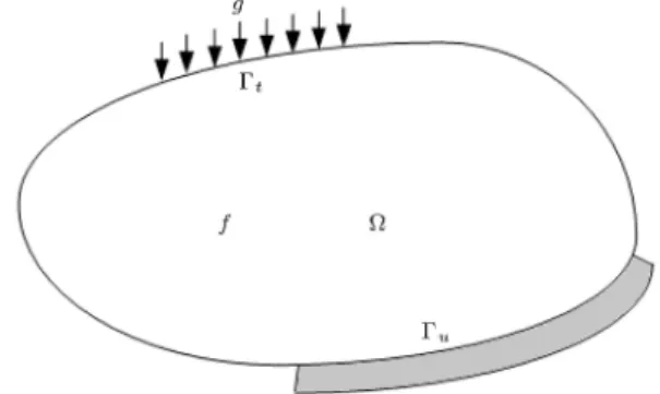
Now, consider a domain of rigid-perfectly plastic body, , with boundary (e.g., = u + t)
shown in Figure 1, and let (f; g) denote the external loading. Under these conditions, the objective of a lower bound calculation is to nd a stress distribution, which satises equilibrium throughout , balances the boundary conditions on , violates the yield criterion
Figure 1. Rigid-perfectly plastic body under external loading.
in no way, and maximizes the integral:
Q = Z
gd + Z
fd; (1)
where functional Q depends on the case which is investigated.
To apply the above formulation, the stress eld must be discretized and the admissibility conditions must be satised for the discretized eld.
2.1. Discretization tool
By the application of mesh-free method as a discretiza-tion tool, the problem domain can be just simulated by a nite number of nodes. An inuence domain is dened around each node (see Figure 2) and continuous stress function (X) is expressed as follows:
(X) = (X)s= N
X
i=1
i(X)i; (2)
where:
s= [1; 2; :::; N]T; (3)
is a vector, consisting of (X) values at N discrete nodes located in the support domain of typical point X, and:
(X) = [1(X); 2(X); :::; N(X)] ; (4)
is a matrix that contains the Shepard's shape functions for N local nodes, in which i(X) is as follows [17]:
i(X) = j6=ir a j
PN
k=1j6=kraj
j = 1; 2; :::; N; (5)
where rj indicates the spatial distance between point
X and node Xj. a is a positive exponent which can
aect the shape of interpolated function. Gordon and Wixom [18] suggested a > 1 for smoothness of the interpolated functions.
The shape functions constructed by the Shep-ard method have the Kronecker delta function prop-erty [18], which allows for the simple imposition of the boundary conditions. Besides, the interpolated values by the Shepard method always lie between the maximum and minimum nodal values used for the interpolation process [18]. The derivatives of Shepard's shape functions also satisfy the consistency conditions in two dimensions as follows [19]:
N
X
i=1
i;x= 0; N
X
i=1
i;y= 0; (6a)
N
X
i=1
i;xxi= 1; N
X
i=1
i;yxi= 0; (6b)
N
X
i=1
i;xyi = 0 N
X
i=1
i;yyi= 1; (6c)
where a comma denotes the derivative with respect to the following subscript.
2.2. Admissibility conditions
In every lower bound solution, the equilibrium equa-tions, the boundary condiequa-tions, and the non-violating yield conditions must be satised. Each condition is briey discussed in the following sub-sections. For more details, the reader is referred to [9].
2.2.1. Equilibrium equations
The equilibrium equations are stated as follows: @ij
@xj + bi= 0; (7)
where ij and bi are the stress tensor and body force
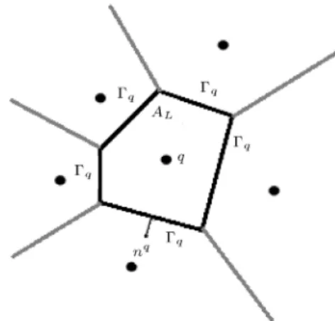
vector, respectively. By dening Voronoi cell around each node and smoothing the stress gradient in the cell, Eq. (7) converts to:
1 AL
Z
L
ijnjd + bi= 0; (8)
where ALis the area of Voronoi cell, Lis the boundary
of Voronoi cell, and nj is the normal unit vector in j
Figure 3. Voronoi cell around node q.
direction (see Figure 3). By the application of Eq. (2) into Eq. (8), the discretized form of Eq. (8) can be written as:
X
z2K
1 AL
Z
L
z(X)njij(Xz)d + bi = 0; (9)
where ij(X) is the stress value at spatial coordinate X,
z(X) is the shape function dened by Eq. (3), ij(Xz)
is the nodal stress value at spatial coordinate Xz, and
K is the group of nodes located at the inuence domain of point X.
Finally, satisfaction of Eq. (9) at all Voronoi cells gives the following matrix form:
Aeq = Beq; (10)
where Aeq is the coecient matrix, is the matrix
that consists of stress tensors, and Beq is the body
force matrix.
2.2.2. Boundary conditions
As the Shepard's shape functions have the Kronecker delta function property, the tractions at the bound-aries can be imposed easily by considering segments with constant stress. In this regard, the gradient of smoothed stress along each segment of boundary with constant stress equates to zero and the values of stresses are imposed at the boundary nodes. These manipulations lead to a system of equations as follows: Abo = Bbo; (11)
where Abois the coecient matrix and Bbois the vector
of specied values of stresses along the boundary. 2.2.3. Non-yielding condition
As the interpolated values (i.e., stresses) by Shepard method always lie between the maximum and minimum nodal values [18], it is sucient for the yield condition to be checked only at the nodes. Considering the
Mohr-Coulomb failure criterion in 2D space X = (x; y), under plane strain condition, the yield function can be written as follows:
F =q(xx yy)2+ (2xy)2+ (xx+ yy) sin '
2C cos '; (12)
where C and ' are cohesion and friction angles of the soil, respectively. For plastically admissible stress eld, we have:
F 0; (13)
at every point in the problem domain.
3. Establishment of the optimization problem Considering the objective function and the required constraints, the lower bound limit analysis problem can be expressed as a non-linear optimization problem in the following format:
Minimize Q()
Subject to: Atot = Btot;
F () ; 0 (14)
where Atot and Btot are the matrices obtained by
the assemblage of equilibrium and boundary condition constraints.
As it is shown, the objective function and equality constraints arising from the equilibrium and boundary conditions are linear equations, with the only non-linearity arising from the yield inequalities. To avoid the local smoothing of the yield function, the second-order cone programming approach [20] is used to solve the obtained non-linear optimization problem. In this context, X = (x; y) in two dimensions, and stress space = [xx yy xy]T converts to equivalent stress space
S = [mSxx Sxy]T as follows [21]:
S = P 1; (15)
P = 2
411 11 00 0 0 1 3
5 : (16)
Using the obtained equivalent stress space, the yield function (i.e., Eq. (12)) can be re-written as follows:
q S2
xx+ Sxy2 + msin ' C cos ' 0: (17)
By introducing variable Z as:
Z = C cos ' msin '; (18)
the yield function becomes: q
S2
xx+ S2xy Z; (19)
and thus, the nonlinear optimization problem can be re-written in the form of second-order cone program-ming problem as follows:
Minimize Q(S) subject to : A
totS = Btot
q S2
xx;i+ Sxy;i2 Zi i = 1; :::; N; (20)
where subscript i denotes the node at which the non-yielding condition should be checked and N indicates the total number of nodes. A
tot and Btot are the
modied versions of matrices Atot and Btot to be
consistent with the new stress space, respectively. The obtained optimization problem is solved by the interior point method [22].
4. Adaptive procedure
To improve the eciency of computations, a technique is proposed here to develop adaptive conguration of nodes. An important part of any adaptive procedure is to establish an error estimator with which the renement strategy can be dened.
4.1. Error estimation
The method proposed by Liu et al. [23] is used here to dene an error estimator in two dimensions. On this subject, using Eq. (2), the dierence between the derivatives of approximated function, h
;x(X), and real
function, ;x(X), can be written as follows:
h
;x(X) ;x(X) = N
X
i=1
i;x(X)(Xi) ;x(X): (21)
Using Taylor series expansion in two dimensions, X = (x; y), (Xi) may be expanded around X:
(Xi) =(X) + ;x(X)(xi x) + ;y(X)(yi y)
+12;xx(X)(xi x)2+ ;xy(X)(xi x)
(yi y) +12;yy(X)(yi y)2+ O(h3): (22)
Substituting Eq. (22) into (21) and ignoring higher order terms, we can write h
h
;x(X) ;x(X) = N
X
i=1
i;x(X)(Xi) ;x(X)
= (X)
N
X
i=1
i;x(X)
+ ;x(X) N
X
i=1
i;x(X)(xi x) 1
!
+ ;y(X) N
X
i=1
i;x(X)(yi y)
+12;xx(X) N
X
i=1
i;x(xi x)2
+ ;xy(X) N
X
i=1
i;x(X)(xi x)(yi y)
+12;yy(X) N
X
i=1
i;x(X)(yi y)2: (23)
Eqs. (6a), (6b), and (6c) simplify Eq. (23) to:
h
;x(X) ;x(X) = 12;xx(X) N
X
i=1
i;x(xi x)2
+ ;xy(X) N
X
i=1
i;x(X)(xi x)(yi y)
+1
2;yy(X)
N
X
i=1
i;x(X)(yi y)2: (24)
Therefore: h
;x(X) ;x(X) 12j;xx(X)j
N X i=1
i;x(xi x)2
+ j;xy(X)j N
X
i=1
i;x(X)(xi x)(yi y)
+1
2j;yy(X)j XN
i=1
i;x(X)(yi y)2:
(25) Since all of the shape functions have a compact support (i.e., inuence domain), there exists constant RI, such
that for any X = (x; y):
jxI xj < RI; jyI yj < RI: (26)
The value of RI can be estimated by:
RI = dc; (27)
where is a dimensionless coecient that lies between 2 and 3, and dc is a characteristic length which is
associated with the nodal spacing near the point. If the nodes are uniformly distributed, dc is simply the
distance between two neighboring nodes. In case where the nodes are non-uniformly distributed, dc can be
dened as an average nodal spacing in the inuence domain. There is also a bound on the values of the shape functions in each inuence domain, and hence the following relation exists:
N X i=1 i;x(X)
< ; (28)
where is a bounded constant.
Considering Eqs. (25) to (27), L2-norm of error
estimate can be written as: jjh
;x(X) ;x(X)jjL2() C1jj1
2;xx(X) + ;xy(X) +12;yy(X)jjL2(); (29)
where C1 is a constant dened as:
C1= hR2I: (30)
4.2. Renement criteria
Based on the error estimate discussed in Section 4-1, the local error is computed at each Voronoi cell from the obtained stress eld. This local error is controlled by a dimensionless user-dened error tolerance value as follows:
jj12;xx(X) + ;xy(X) +21;yy(X)jjL2() : (31)
To calculate ;(X) numerically, a smoothing
tech-nique, similar to the one introduced by Chen et al. [24], has been used. In this regard:
~;(X) = A1 L
Z
L
;(X)d; (32)
where ;(X) can be written in a discrete form by the
application of Shepard's shape functions as follows: ;(X) =
X
Z2K
Z;(XZ); (33)
where K is the group of nodes located in the support domain of point X. In the above equation, the smoothed version of shape function's derivative (i.e., ~Z;) can be used instead of Z;. The smoothed
version over a Voronoi cell (i.e., L) can be obtained
~Z;(Xq) =A1 L
I
q
Z;(Xq)n
+ Z;(Xq)n
d ; (34)
where:
~Z;(Xq) = A1 L
I
q
(Z(Xq)n) d
= A1
L Ns
X
k=1
nD
LD+ nD+1 LD+1
Z(XD+1q ); (35)
where Ns is the total number of segments of Voronoi
cell that contains node q; XD
q and XD+1q are the two
end points of boundary segment D
k; and LD is the
length of D
k. nDx and nDy are, respectively, x and y
components of the normal vector to D k.
Using Eqs. (31) to (35), the local error at each Voroni cell can be estimated directly. If this local error exceeds predened value, , new nodes are added at the vertices of specied Voronoi cell. The process is repeated for each Voronoi cell until all local errors become smaller than pre-dened error tolerance, .
5. Numerical study
The eciency of the proposed adaptive method is investigated here by solving some examples on purely cohesive and cohesive-frictional soils. In all examples, the shape functions are constructed by considering a circle support domain around each node and sucient number of nodes covered by the support domain in an automatically self-tuned value of radiuses devised in the code. The boundaries of the models are also suciently distant from the loading area to ensure that the discretized domain always contains the entire plastic zones.
5.1. Example (1): Smooth strip footing resting on purely cohesive soil
The exact collapse pressure for a smooth strip footing resting on weightless purely cohesive soil is given by the well-known Prandtl solution [25] as qult = 5:14C, where
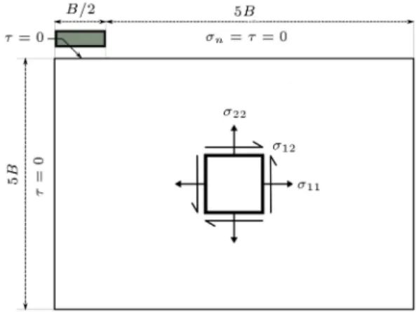
C is the soil cohesion. The geometry and boundary conditions used to analyze this problem are shown in Figure 4. Due to the symmetry, only one half of the geometry is modeled in the numerical study.
Both uniform and adaptive nodal renement tech-niques are used in the proposed mesh-free lower bound method to nd the collapse load. Uniform nodal renement is carried out by considering four mesh-free models shown in Figure 5. The obtained results from
Figure 4. The geometry and boundary conditions for undrained loading problem.
Figure 5. Uniform renement with (a) 196, (b) 379, (c) 726, and (d) 1117 nodes (undrained loading problem).
lower bound limit analysis with linear and nonlinear programming are shown in Table 1. As shown, the application of nonlinear programming improves the accuracy of results, and that all evaluated values are lower than those of the exact solution are. It is also evident that the higher density of nodes provides better results.
In order to assess the eciency of the proposed adaptive procedure, the model shown in Figure 5(b) is selected as the base model to carry out adaptive nodal renement. Once the optimization process is nished, the local error of the obtained stress eld is computed at each Voronoi cell. In the regions where error exceeds the pre-dened tolerance, new nodes are added at the vertices of the cell. It is noteworthy that based on the numerical tests performed by Le et al. [16], the optimum value of pre-dened local error tolerance is selected as 0.001. The restructuring process continues until the error tolerance is satised at all nodes. As depicted in Figure 6, the density of nodes
Table 1. Normalized collapse pressure (qult
C ) obtained using uniform renement (undrained loading problem).
Model shown in
Number of nodes
Exact solution
Lower bound (linear programming [9])
Lower bound (nonlinear
programming)
Figure 5(a) 196 5.14 3.140 3.160
Figure 5(b) 379 5.14 4.351 4.378
Figure 5(c) 726 5.14 4.678 4.709
Figure 5(d) 1117 5.14 4.939 4.967
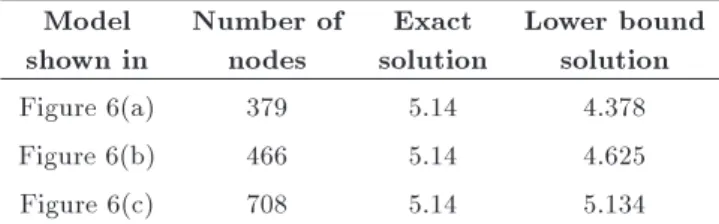
Figure 6. Adaptive renement with (a) 379, (b) 466, and (c) 708 nodes (undrained loading problem).
Table 2. Normalized collapse pressure (qult
C ) obtained
using adaptive renement (undrained loading problem). Model
shown in
Number of nodes
Exact solution
Lower bound solution
Figure 6(a) 379 5.14 4.378
Figure 6(b) 466 5.14 4.625
Figure 6(c) 708 5.14 5.134
increases in the vicinity of high-stress gradient beneath the footing, where the plastic points are expected to take place. Table 2 shows the results of dierent steps of adaptive analysis, and a comparison between the results of uniform and adaptive nodal renement is depicted in Figure 7. It can be seen that the proposed adaptive procedure converges to the exact solution with the smaller number of nodes, conrming the eciency of the method.
5.2. Example (2): Smooth strip footing resting on cohesive-frictional soil
In order to study the eciency of the proposed adap-tive procedure for cohesive-frictional soils, the drained
Figure 7. Comparison between normalized collapse pressures obtained using uniform and adaptive renement (undrained loading problem).
loading of a smooth strip footing is investigated here. According to [26], the ultimate load of a smooth strip foundation resting on a semi-innite cohesive-frictional soil can be estimated by:
qf = CNc+ 0:5BN; (36)
Nc= (Nq 1) cot '0; (37)
Nq = exp( tan '0) tan2(4 +' 0
2 ); (38) where qf, C, and '0 are the ultimate pressure, the soil
cohesion, and the eective internal friction angle of soil, respectively. B and are the width of foundation and the soil unit weight, respectively. N is evaluated by
the well-known Brinch Hansen [27] formula as follows: N = 1:5(Nq 1) tan '0: (39)
As known, by increasing the value of '0, the extent of
failure zone beneath the foundation increases. Thus, in the present example, the boundaries of the model in both directions are extended to the distance of 10B from the edges of the foundation to ensure that the considered domain encloses the failure zone, and that there is no intersection between the plastic zone
Figure 8. Adaptive renement with (a) 3660, (b) 5100, and (c) 10193 nodes (drained loading problem).
and the domain boundaries. The problem is solved for B=2C = 1 and '0 = 30 to account for the
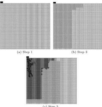
presence of soil unit weight, cohesion, and friction angle simultaneously. As depicted in Figure 8, the adaptivity analysis begins with a uniform arrangement of nodes located at a distance of 0.35 m from each other. The total number of nodes in the rst model is 3660. By the continuation of adaptive renement, the number of nodes gets into 5100 and 8193 for the third and fth steps of analysis, respectively. The comparison between the Brinch Hansen's solution and the results obtained at dierent steps of the adaptivity analysis (depicted in Table 3) shows that the adaptive procedure can provide very good results for a problem associated with the cohesive-frictional soil.
5.3. Example (3): Trapdoor problem
Some practical problems, such as the stability of temporary tunnel roofs or abandoned mining areas, are simply simulated by plane strain trapdoor problem. In this problem, a layer of purely cohesive soil, with undrained shear strength, Su, and thickness H, rests
on a trapdoor of width B (Figure 9). The trapdoor itself and stratum underlying the soil layer are assumed
Figure 9. Trapdoor problem.
to be non-yielding materials. As shown in Figure 9, in stable condition, externally applied stress t must be
suciently high to resist the active failure of the soil above the trapdoor. The stability of trapdoor is usually studied by dening a stability number as follows:
N = (H + s t)=Su; (40)
where N, , H, and Su are the stability number, soil
unit weight, soil layer thickness, and undrained shear strength of soil, respectively. Stresses s and t are
depicted in Figure 9. The stability number is a function of H=B value; however, the exact value of stability number cannot be found strictly, and upper or lower bound solutions are presented by some researchers [28-30].
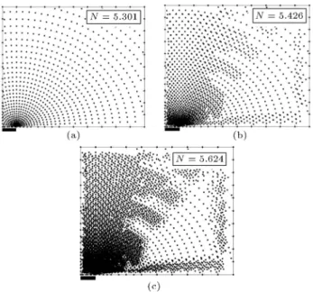
In this example, the lower bound values have been found for the stability numbers of weightless soil trapdoor problem with H=B = 5 and smooth interface of soil and trapdoor. According to the authors' survey, the best lower and upper bound solutions to the stability number of this problem are found by Sloan et al. [30] and the values are, respectively, 5.62 and 6.16. As depicted in Figure 10, three successive mesh-free models with adaptive renement are considered. In these models, a major increase in the density of nodes occurs in the active failure zone above the trapdoor where it is expected of the soil to behave plastically. The stability numbers of all models are also shown in the gure. As it is obvious, the lower bound solutions are all lower than the upper bound value, and the nal result is in very good agreement with that of the nite-element limit analysis of Sloan et al. [30].
Table 3. Ultimate load obtained using adaptive renement (drained loading problem). Model
shown in
Number of nodes
Brinch Hansen's solution [27]
Lower bound solution
Figure 8(a) 3660 45.21 38.68
Figure 8(b) 5100 45.21 41.61
Figure 10. Adaptive renement with (a) 830, (b) 990, and (c) 3460 nodes (trapdoor problem).
6. Conclusion
An adaptive mesh-free lower bound limit analysis formulation was proposed for the prediction of limit loads in soil mechanics problems under plane strain condition. In the presented approach, the lower bound theorem of classical plasticity was combined with a conforming mesh-free technique to render nonlinear discretized optimization problem. This problem con-verted to a second-order cone programming problem and was solved by the interior point method. To improve the computational eciency of the proposed method, an adaptive approach based on Taylor series expansion was oered. In this approach, h-renement was used and the nodes were adaptively added to the vertices of Voronoi cells. The results of adaptive anal-ysis for purely cohesive soil and cohesive-frictional soil revealed that the addition of nodes mainly occurred in the expected plastic zones and the acceptable estimates of lower bound for limit load could be obtained by relatively small number of nodes. Besides, it seems appropriate for the proposed method to be extended for de-remeshing technique in future research studies, where the nodes are removed in the areas with very low error estimate. It is worth mentioning that due to the relaxation occurred during the process of stress gradient smoothing, the proposed method cannot be guaranteed to produce rigorous lower bound solutions. However, for all problems investigated, the obtained results values were lower than known exact solutions.
References
1. Drucker, D.C., Prager, W. and Greenberg, H.J. \Ex-tended limit design theorems for continuous media",
Quarterly Journal of Applied Mathematics, 9(4), pp. 381-389 (1952).
2. Sloan, S.W. \Geotechnical stability analysis", Geotech-nique, 63(7), pp. 531-572 (2013).
3. Chen, S., Liu, Y. and Cen, Zh. \Lower-bound limit analysis by using the EFG method and non-linear programming", International Journal for Numerical Methods in Engineering, 74, pp. 391-415 (2008).
4. Chen, S., Liu, Y. and Cen, Zh. \Lower-bound shake-down analysis by using the element free Galerkin method and non-linear programming", Computer Methods in Applied Mechanics and Engineering, 197, pp. 3911-3921 (2008).
5. Le, C.V., Gilbert, M. and Askes, H. \Limit analysis of plates using the EFG method and second-order cone programming", International Journal for Numerical Methods in Engineering, 78(13), pp. 1532-1555 (2009).
6. Le, C.V., Gilbert, M. and Askes, H. \Limit analysis of plates and slabs using a meshless equilibrium formula-tion", International Journal for Numerical Methods in Engineering, 83(13), pp. 1739-1758 (2010).
7. Liu, F. and Zhao, J. \Upper bound limit analysis using radial point interpolation meshless method and nonlinear programming", International Journal of Me-chanical Sciences, 70, pp. 26-38 (2013).
8. Binesh, S.M. and Raei, S. \Upper bound limit analysis of cohesive soils using mesh-free method", Geomechan-ics and Geoengineering: An International Journal, 9(4), pp. 265-278 (2014).
9. Binesh, S.M. and Gholampour, A. \Mesh-free lower bound limit analysis", International Journal of Com-putational Methods, 11(6), p. 1350105 (2014).
10. Borges, L.A., Zouain, N., Costa, C. and Feijoo, R. \An adaptive approach to limit analysis", International Journal of Solids and Structures, 38, pp. 1707-1720 (2001).
11. Christiansen, E. and Pedersen, O.S. \Automatic mesh renement in limit analysis", International Journal for Numerical Methods in Engineering, 50, pp. 1331-1346 (2001).
12. Lyamin, A.V., Sloan, S.W., Krabbenhoft, K. and Hjiaj, M. \Lower bound limit analysis with adap-tive remeshing", International Journal for Numerical Methods in Engineering, 63, pp. 1961-1974 (2005).
13. Ciria, H., Peraire, J. and Bonet, J. \Mesh adaptive computation of upper and lower bounds in limit anal-ysis", International Journal for Numerical Methods in Engineering, 75, pp. 899-944 (2008).
14. Munoz, J., Bonet, J., Huerta, A. and Peraire, J. \Upper and lower bounds in limit analysis: adaptive meshing strategies and discontinuous loading", Inter-national Journal for Numerical Methods in Engineer-ing, 77, pp. 451-501 (2009).
15. NguyenXuan, H. and Liu, G.R. \An edgebased -nite element method (ES-FEM) with adaptive scaled-bubble functions for plane strain limit analysis", Com-puter Methods in Applied Mechanics and Engineering, 285, pp. 877-905 (2015).
16. Le, C.V., Askes, H. and Gilbert, M. \Adaptive element-free Galerkin method applied to the limit analysis of plates", Computer Methods in Applied Me-chanics and Engineering, 199, pp. 2487-2496 (2010).
17. Shepard, D. \A two-dimensional interpolation function for irregularly-spaced data", Proc. ACM Nat. Conf., pp. 517-24 (1968).
18. Gordon, W. and Wixom, J. \Shepard's method of metric interpolation to bivariate and multivariate in-terpolation", Mathematics of Computation, 32(141), pp. 253-264 (1978).
19. Krongauz, Y. and Belytschko, T. \Consistent pseudo-derivatives in meshless methods", Computer Methods in Applied Mechanics and Engineering, 146, pp. 371-386 (1997).
20. Lobo, M.S., Vandenberghe, L. and Boyd, S. \Appli-cations of second-order cone programming", Linear Algebra and Its Application, 284, pp. 193-228 (1998).
21. Makrodimopoulos, A. and Martin, C.M. \Lower bound limit analysis of cohesive-frictional materials using second-order cone programming", International Jour-nal for Numerical Methods in Engineering, 66(4), pp. 604-634 (2006).
22. Andersen, E.D., Roos, C. and Terlaky, T. \On imple-menting a primal-dual interior-point method for conic quadratic", Mathematical Programming, 95, pp. 249-277 (2003).
23. Liu, W., Li, S. and Belytschko, T. \Moving least square reproducing kernel methods: (i) methodology and con-vergence", Computer Methods in Applied Mechanics and Engineering, 139, pp. 159-193 (1996).
24. Chen, J.S., Wu, C.T., Yoon, S. and You, Y. \A stabi-lized conforming nodal integration for Galerkin Mesh-free methods", International Journal for Numerical Methods in Engineering, 50, pp. 435-466 (2001).
25. Prandtl, L. \Uber die Eindringungs-festigkeit (Ha'rte) plastischer Bausoe und die Festigkeit von Schneiden", Zeitschrift fur angewandte Mathematik und Mechanik, 1(1), pp. 15-20 (1921).
26. Terzaghi, K., Theoretical Soil Mechanics, John Wiley & Sons, New York (1943).
27. Brinch Hansen, J., A Revised and Extended Formula for Bearing Capacity, Bulletin of Danish Geotechnical Institute, 28, pp. 5-11 (1970).
28. Davis, E.H. \Theories of plasticity and the failure of soil masses", In Soil Mechanics-Selected Topics, Ch. 6, Ed. I. K. Lee. London: Butterworths (1968).
29. Gunn, M.J. \Limit analysis of undrained stability problems using a very small computer", Proc. Symp. on Computer Applications to Geotechnical Problems in Highway Engineering, Cambridge University, Cam-bridge, England, pp. 5-30 (1980).
30. Sloan, S.W., Assadi, A. and Purushotaman, N. \Undrained stability of a trapdoor", Geotechnique, 40(1), pp. 45-62 (1990).
Biographies
Seyyed Mohammad Binesh was born in 1978. He received his BS degree in Civil Engineering in 2000 and MSc and PhD degrees in 2002 and 2008, respectively, in Geotechnical Engineering, from Shiraz University, Iran. He is currently Associate Professor with the Civil and Environmental Department, Shiraz University of Technology, Shiraz, Iran. His research interests include numerical methods, such as nite element and mesh-free methods, limit load analysis in soil mechanics, laterally loaded piles and rock mechanics.
Sara Rasekh was born in 1986. She received her BS degree in Civil Engineering from Mohaghegh Ardabili University, Iran, in 2010, and her MSc degree in Geotechnical Engineering from Shiraz University of Technology, Iran, in 2013. Her research interests include lower bound determination is soil mechanics problems and non-linear programming.