Sharif University of Technology
Scientia IranicaTransactions B: Mechanical Engineering http://scientiairanica.sharif.edu
Numerical simulations of gas-liquid-particle ows in
three-phase slurry reactors under gravity variation
X. Zhang
a,b;and G. Ahmadi
ca. International Doctoral Innovation Centre, University of Nottingham Ningbo China, 199 Taikang East Road, 315100 Ningbo, China.
b. Research Center for Fluids and Thermal Engineering, University of Nottingham Ningbo China, 199 Taikang East Road; 315100 Ningbo, China.
c. Department of Mechanical and Aeronautical Engineering, Clarkson University, Potsdam, New York, USA. Received 20 February 2018; accepted 18 August 2018
KEYWORDS Numerical simulations; Gas-liquid-particle; Three-phase; Slurry reactors; Gravity variation.
Abstract. Numerical simulations of three-phase gas-liquid-particle ows under 1 g and 2 g gravitational conditions were performed with an Eulerian-Lagrangian method. In this study, the liquid was treated as a continuous phase and modeled by a volume-averaged system of governing equations. Bubbles and particles were modeled as discrete phases using Lagrangian method. Drag, lift, buoyancy, and virtual mass forces were included in the Lagrangian equation. Bubbles were treated as spherical without shape variations. The two-way coupling between bubble-liquid and particle-liquid was included, and interactions between bubble-bubble and particle-particle were considered with the hard sphere model. Particle-bubble interactions and bubble coalescences were also included in the analysis. The results under 1 g normal gravity condition were compared with the available experimental data in earlier simulation, resulting in good agreement. The transient ow characteristics of the three-phase ow under 1 g and 2 g gravitational conditions were studied, and the eects of gravity were analyzed. The results show that gravity has magnicent eect on the ow characteristics of three-phase gas-liquid-particle ows in bubble columns. The three-phase velocities under higher gravity are larger than those of the ow under normal gravity are. The ow under higher gravity develops fast. Bubbles and bubble volume fraction in the higher gravity ow are smaller.
© 2018 Sharif University of Technology. All rights reserved.
1. Introduction
Gas-liquid-particle three-phase bubbly ows with liq-uids, bubbles, and solid particles are widely used in many industrial applications [1]. A typical example is three-phase slurry reactors in coal conversion processes in synthetic liquid fuel production. A good
understand-*. Corresponding author. Tel.: +86 (0) 574 8818 0000-8312; Fax: +86 (0) 574 8818 0175
E-mail address: [email protected] (X. Zhang)
doi: 10.24200/sci.2018.20892
ing of three-phase ow characteristics is critical to the optimization of three-phase slurry reactors. However, with many unresolved issues, the three-phase slurry reactor technology is still not matured. For example, the eects of gravity variation on the three-phase ow characteristics are not clear. It plays an important role in air revitalization and purication devices vital to NASA's long duration human space travel.
Eulerian-Eulerian and Eulerian-Lagrangian ap-proaches are the most widely used two apap-proaches to modeling multiphase ows. The Eulerian-Eulerian approach uses many empirical constitutive equations, and both continuous and discrete phases are treated as continuum media whose properties are analogous
to those of a uid. Therefore, the accuracy of this approach is closely related to the empirical constitutive equations used. The approach has limitations to predict certain discrete phase characteristics including particle size eect, particle agglomeration, and bub-ble coalescences. The Eulerian-Lagrangian approach applies a continuum description for the liquid phase and tracks the bubbles and particles with Lagrangian trajectory method that usually requires extensive com-putation time, yet only involves a smaller number of empirical equations and can provide detailed informa-tion on discrete phase.
The Eulerian-Lagrangian approach is widely used in two-phase ows. For gas-liquid bubbly ows, Delnoij et al. [2,3] developed an Eulerian-Lagrangian model for a bubble column operating in the homogeneous ow regime. Their study considered bubble-bubble interactions, but ignored bubble coalescences. Lain et al. [4,5] provided an Eulerian-Lagrangian approach with turbulence included using the k " turbulence model; however, they neglected the eect of phase volume fractions. Lapin and Lubbert [6] carried out Eulerian-Lagrangian simulations of slender bubble columns with bubble-bubble interactions neglected. They found that the ow moved downwards near the axis and rose close to the wall in the lower part of the column; however, the trend was opposite in the upper part of the column. Besbes et al. [7] performed a three-dimensional Eulerian-Lagrangian simulation with a k " turbulence model and two-way coupling; in addition, they carried out an experimental study using the Par-ticle Image Velocimetry technique (PIV) for the ow in a needle sparger rectangular bubble column. They found that stronger bubble plume velocity oscillations were located near the entrance zone and were brought about by the addition of shear-induced turbulence due to an oscillating bubble plume. Lau et al. [8] developed an Eulerian-Lagrangian model to predict the bubble size distribution in turbulent bubbly ows in a square bubble column with bubble-bubble collisions and co-alescence as well as bubble break-up included. Tyagi and Buwa [9] reported a numerical study of dispersed gas-liquid ow in a small rectangular bubble column using Eulerian-Lagrangian approach to investigate the eect of bubble size distribution and drag as well as lift forces on the ow properties. Xue et al. [10,11] reported on a study concerning the performance of the soft-sphere model in gas-liquid systems, and showed that the soft-sphere model was also suitable for simulations of liquid ows. Masterov et al. [12] studied gas-liquid ows in a square bubble column using Detached Eddy Simulation and Eulerian-Lagrangian approach.
Many works have been done in numerical studies on gas-solid ows. Ahmadi [13] reviewed computa-tional and analytical models for particle transport and deposition in turbulent ows. Nikbakht et al. [14]
reported on an axisymmetric model for nano-particle beam focusing in aerodynamic lenses.
Numerical studies on three-phase liquid-gas-solid ows are limited. Gidaspow et al. [15] devel-oped a model for three-phase-slurry hydrodynamics. Grevskott et al. [16] reported on a two-uid model for three-phase bubble columns in cylindrical coordi-nates including a k " turbulence model and bubble-generated turbulence. Mitra-Majumdar et al. [17] reported on a model to examine the structure of three-phase ows through a vertical column. They included the particle eects on bubble motions and suggested new correlations for the drag between the liquid and the bubbles. Wu and Gidaspow [18] carried out a simulation of gas-liquid-slurry bubbly ows using the kinetic theory of granular ows for particle collisions. Padial et al. [19] performed simulations of three-phase ows in a three-dimensional draft-tube bubble column using a nite-volume technique. Gamwo et al. [20] reported on a model of a chemically active three-phase slurry reactor for methanol synthesis. Li and Zhong [21] studied the gas-liquid-solid three-phase ow in bubble columns using a three-dimensional time-dependent Eulerian-Eulerian-Eulerian three-uid ap-proach. Bogner et al. [22] performed a direct numerical simulation of liquid-gas-solid ows with a free surface Lattice Boltzmann method. All the above models are based on Eulerian-Eulerian approach. Simulations of gas-liquid-solid ows using an Eulerian-Lagrangian approach are rather limited. Zhang [23] performed a series of simulations of a three-phase ow using Volume-Of-Fluid (VOF) method for the liquid and the gas phases and a Lagrangian method for particles. His studies were limited to a small number of bubbles. Bourloutski and Sommerfeld [24] carried out simula-tions of dense gas-liquid-solid ows with standard k " turbulence model, but neglected bubble coalescences, bubble-bubble collision, and particle-particle collision. Sun and Sakai [25] performed three-dimensional sim-ulations of gas-solid-liquid ows using an Eulerian-Lagrangian approach associated with VOF method.
Zhang and Ahmadi [26] reported on a model for simulations of gas-liquid-particle ows using an Eulerian-Lagrangian approach. In their study, the bubbles and particles were treated as the dispersed discrete phases, and their motions were described using the Lagrangian trajectory method. Two-way interac-tions among liquid-particles, liquid-bubbles, particle-particle, bubble-bubble, and particle-bubble as well as bubble coalescences were included. The simulation results were in good agreement with the experimental data of Delnoij et al. [2]. Based on this approach, Zhang and Ahmadi [27] studied the eects of particle density on gas-liquid-solid ows using a parcel method to account for particle load.
model was used, and a sample case with normal gravity was analyzed rst. Then, the inuences of the gravity variation on operation of the column were analyzed by increasing 1 g normal gravity to 2 g gravitational condition.
2. Governing equations and models
Zhang and Ahmadi [26] provided the detailed informa-tion on governing equainforma-tions and model assumpinforma-tions. Thus, only an outline of the key equations is presented here.
2.1. Fluid phase hydrodynamics
The liquid phase is described by volume-averaged, incompressible transient Navier-Stokes equations. The volume-averaged continuity equation and momentum equation are given as follows:
@ ("ff)
@t + r ("ffuf) = 0; (1) and:
f"fd (udtf)= "frp + r ("ff) + fg"f+ P; (2)
where "f is the liquid phase volume fraction, f is
the liquid phase density, uf is the uid phase average
velocity, p is the pressure, g is the acceleration of gravity, P is the interaction momentum per unit mass transferred from the discrete phases, and f is the
liquid phase viscous stress tensor, which is assumed to follow the general Newtonian uid form described by:
f = 23f(r uf) I + f
(ruf) + (ruf)T
; (3) where f is the liquid dynamic viscosity.
2.2. Dispersed phase dynamics
The bubbles and particles are treated as discrete phases, and their motions are given by Newton's second law, i.e.:
mddudtd = Fd+ Fb+ Fvm+ Fl+ FInt; (4)
where md and ud are, respectively, mass and discrete
phase velocity. The terms on the right-hand side of Eq. (6) are, respectively, drag, buoyancy, virtual mass, lift and interaction forces. Herein, interaction force FInt
includes particle, bubble-bubble, and particle-bubble collisions.
The drag force, Fd, is given as follows:
Fd=
(
0:125fCDd2djuf udj (uf ud) ; Red 1
dfdd(uf ud); Red< 1 (5)
where dd is the discrete phase diameter, d is a phase
coecient whose value is 2 for bubble and 3 for rigid particle to account for the variation of the Stokes drag
force for bubbles and particles in low Reynolds number ows. In Eq. (5), Red is the discrete phase Reynolds
number given by:
Red= fddjuf udj
f : (6)
In addition, CDis the drag coecient given by:
CD= fdRe24
d; (7)
where fd is given by:
fd=
1 + 0:15Re0:687
d ; Red 1000
0:0183Red; Red> 1000 (8)
In Eq. (4), Fl is the Saman lift force given by:
Fl= 1:61d2d(ff)0:5j!fj 0:5[(uf ud) !f] ; (9)
where ow vorticity !f is dened as follows:
!f = r uf: (10)
In Eq. (4), Fbis the buoyancy force given by:
Fb= dd 3
6 (f d)g; (11) where d is the discrete phase density.
In Eq. (4), Fvmis the virtual mass force described
by:
Fvm= 121 d3dfdtd(ud uf): (12)
2.3. Discrete phase collisions and two-way coupling
Collisions between Bubble-bubble and particle-particle are considered in this study using a hard sphere collision model based on the model developed by Hoomans et al. [28]. However, the eects of the rotation of bubbles and particles were neglected in the analysis. Restitution coecients of 0.2 and 0.5 are used, respectively, for the collision between bubble-bubble and particle-particle. Friction coecients of 0.02 and 0.1 are assumed for bubbles and particles, respectively, and all the bubble-bubble and particle-particle collisions are assumed as binary.
Bubble-particle interactions are considered in the study by assuming that the particles go through the bubbles when bubble-particle collision occurs. Multiple interactions between bubble and particle are included, meaning that, at the same time, more than one particle can enter the same bubble or dierent bubbles. In the present study, bubble coalescences are also included by assuming that two bubbles coalesce upon impact when
the Weber number is less than 0.14, while they bounce back for larger Weber numbers.
Two-way coupling between uid and dispersed phases is included in momentum interaction term, P, from the discrete phase to uid phase. P is the negative of the sum of all forces acting on the particles and bubbles exerted by the uid in a certain Eulerian computation cell. The coupling between bubbles and particles is included in bubble-particle interactions. When a particle enters a bubble, all the forces acting on the particles by the new gaseous environment are calculated with the bubble hydrodynamic properties until the particle leaves the bubble. The exact force with opposite direction is then added to the bubble equation of motion.
2.4. Geometry and boundary conditions
The present study was carried out on a pseudo-two-dimensional bubble column with a rectangular cross-section. Figure 1 shows the schematic of the bubble column. In this setup, bubbles rise through a 25 cm wide, 75 cm high, and 2 cm thick column from 14 uniformly spaced gas inlets located at the center of the column bottom surface. The distance between
Figure 1. Schematic of the pseudo-two-dimensional bubble column.
each of two neighboring inlets is 4 mm. In the simulations, identical geometry was used, and buoyant particles were randomly distributed neutrally in the column at the initial time. The continuous phase was assumed tap water, and its physical properties were kept xed in the simulations. The initial liquid level is 55 cm high, while the gravity varies for dierent cases. Table 1 summarizes the hydrodynamic properties of the dispersed phases for dierent cases studied.
No-slip boundary conditions were applied on three walls of the column for the liquid phase, and an outow condition was assumed at the upper boundary of the column. Bubble-wall and particle-wall collisions were included in the model using a hard sphere collision model derived from the model developed by Hoomans et al. [28]. The wall roughness eects and the rotation of bubbles and particles were ignored. A restitution coecient of 0.5 was used for both bubble-wall collision and particle-wall collision with friction coecients of 0.02 and 0.1 used for bubble-wall collision and particle-wall collision, respectively.
The Marker-And-Cell (MAC) method [29] was used to simulate the column free surface. The details of the boundary conditions for free surface are included in the former paper. A simple model for interaction of bubbles with the free surface is used in this study. In this model, it is assumed that the bubbles that impact the column free surface with Weber number less than 0.28 will break and leave the column, while bubbles impacting at higher Weber numbers will bounce back using the above-mentioned hard sphere model. A restitution coecient of 0.2 was used for bubble-free surface collisions when We > 0:28.
2.5. Numerical procedure
The governing equations of the model were discretized with nite dierence method in a structured equidis-tant staggered grid. A combination of central and donor-cell discretization schemes was used for convec-tive parts, while an explicit time step was used for time updating. Griebel et al. [30] presented detailed information. The model was implemented in a new de-veloped computer code ELM3PF (Eulerian-Lagrangian Method for Three Phase Flow) to simulate three-phase
Table 1. Hydrodynamic parameters for dierent cases. Case number Bubble diameter
(mm)
Supercial gas velocity (mm/s)
Bubble density (kg/m3)
1 1.0 0.25 1.29
2 1.0 0.25 1.29
Case number Particle diameter (mm)
Particle density (kg/m)
Gravity (m/s2)
1 0.25 1000 -9.8
ows. The new code was developed in C from NaSt2D code, which was a code for single-phase ows with free surface developed by Griebel et al. [30]. The new code (ELM3PF) can be used to simulate unsteady, pseudo-two-dimensional three-phase liquid-gas-solid ows with free surface.
The pressure Poisson equations for liquid phase are solved by Successive Over-Relaxation (SOR) method in ELM3PF. For liquid phase calculation, a xed time step t, which is 0.001 s, is used in the study. At rst, the code calculates the liquid phase velocity eld. Then, after obtaining the new liquid velocity eld, the code is used to evaluate the minimum time for next collision, dt, which is the minimum time of all possible collisions. If dt is smaller than t, the code is used to calculate bubble and particle velocities and positions over time duration dt. The next collision process is then analyzed, and the corre-sponding discrete phase velocities after the collision are evaluated. Then, the code computes the next minimum time for collision, and this procedure is repeated until the accumulation of these dt equals t. Thereafter, the forces acting on the bubbles and particles are evaluated and transferred into the momentum equation for the liquid phase. The code then computes the new liquid velocity eld. If minimum collision time dt is larger than t, the code computes the forces acting on the bubbles and particles, transfers these forces into momentum equations for liquid phase, and evaluates the new liquid velocity. In this study, 9940 bubbles and 1000 particles are used. CPU time requirement depends on the number of particles, bubbles, and grid cells. For a typical number of bubbles and particles with a computational grid of 1500 cells, evaluating a second transient behavior of the liquid-gas-solid three-phase ow requires around 4 hours of CPU time on a SUN Ultra10 workstation.
2.6. Eect of grid size
To test the sensitivity of the simulation result to the grid size, the grid size was reduced by a factor of two from 1 cm to 0.5 cm. The results did not show obvious dierences. Therefore, a grid spacing of 1 cm was typically used.
3. Results and discussion
3.1. Development of transient ow structures with normal gravity
At rst, to evaluate the eect of the gravity variation on the three-phase ow characteristics, a sample reference case with normal gravity is studied. The hydrodynamic parameters for the simulation are listed in Table 1 (Case 1). The simulation results under normal gravity in the previous work by Zhang and Ahmadi [26] were
Figure 2. Computed ow structure of the
gas-liquid-particle three-phase ow in normal gravity. (Supercial gas velocity, Us= 0:25 mm/s; initial bubble
size, db= 1:0 mm; and particle size, dp= 0:25 mm.)
Figure 3. Computed snapshots of the bubble velocities of the gas-liquid-particle three-phase ow in normal gravity. (Supercial gas velocity, Us= 0:25 mm/s; initial bubble
size, db= 1:0 mm; and particle size, dp= 0:25 mm.)
compared with the experimental data of Delnoij et al. [2], leading to good agreement.
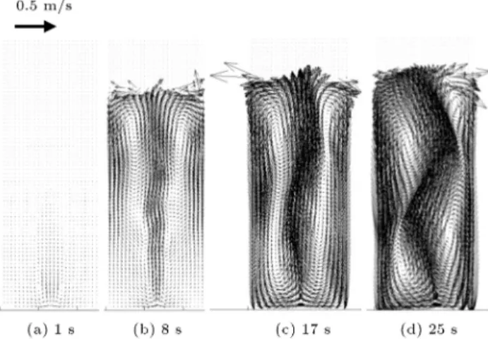
Figure 2 shows the snapshots of the liquid stream traces, the locations of bubbles, and particles at times of 1, 8, 17, and 25 s after initiation of the ow. The small dots in Figure 2 show the liquid phase stream traces, while the small circles and the large circles show the positions of the particles and bubbles, respectively. Figures 3, 4, and 5 show the corresponding velocities of bubbles, liquid, and particles, respectively. The transient ow features can be seen clearly from these gures. Figure 2(a), (b), and (c) show that bubble plume rises rectilinearly along the centerline of the column, and there are two vortices generated behind the plume head, as seen in Figure 4(a), (b), and (c). These vortices are almost symmetric at the beginning, but become non-symmetric with the evolution of the ow, resulting in staggered vortical ows, as shown in Figure 4(d). The bubble plume changes its pattern to S-shape as seen in Figure 2(d) due to these staggered
Figure 4. Computed snapshots of the liquid velocities of the gas-liquid-particle three-phase ow in normal gravity. (Supercial gas velocity, Us= 0:25 mm/s; initial bubble
size, db= 1:0 mm; and particle size, dp= 0:25 mm.)
Figure 5. Computed snapshots of the particle velocities of the gas-liquid-particle three-phase ow in normal gravity. (Supercial gas velocity, Us= 0:25 mm/s; initial
bubble size, db= 1:0 mm; and particle size, dp= 0:25
mm.)
vortices. The moving of these staggered vortices results in the oscillation of the bubble plume. A comparison of Figure 2 and Figure 4 shows that the evolution of the three-phase ow in the column is aected by these time-dependent staggered vortices.
Figure 3(b), (c), and (d) show that bubble upward velocities increase along the column height. The bubble upward velocities attain the maximum at about 0.45 m at 8 s, 0.3 m at 17 s, and 0.25 m at 25 s, respectively. Then, they decrease along the column height because of the increasing liquid drag resulting from the low liquid upward velocity near the free surface. A comparison of Figure 3(b), (c), and (d) shows that bubble maximum upward velocities increase with time. However, the variations of bubble upward velocities with time in other regions of the column are not as large as the increase of the maximum value. Thus, the dierences of the bubble upward velocities along the column height increase with time, which may result in more bubble-bubble collisions and coalescences.
Figures 4 and 5 show that the liquid and particle upward velocities increase along the column height, attaining the maximum at about 0.4 m at 8 s, 0.25 m at 17 s, and 0.2 m at 25 s, respectively and, then, decreasing along the column height. These maximum upward velocities and the dierences of these upward velocities along the column height increase with time, which may result in more particle-particle collision with the development of the ow. Figure 4 shows that due to liquid velocity distribution, the collision mode for discrete-phases is dierent in the top and low parts of the column. Due to the eect of liquid vortices, bubbles and particles in the low part of the column are pushed toward the centerline, which will result in horizontal bubble-bubble and particle-particle collisions. In this region, particles and bubbles are in the acceleration process; particles or bubbles behind cannot easily catch up those above them. Therefore, longitudinal collisions are scarce. In the top part of the column, the liquid velocities push the bubbles and particles toward the sidewall of the column; therefore, horizontal collisions are scarce. However, particles and bubbles in this region are in the deceleration process; thus, longitudinal collisions will play a major role. As for the collisions between bubbles and particles, bubble upward velocities usually are larger than particle veloc-ities are, and longitudinal collisions can occur along the full column height.
The location dierence between the maximum upward velocities of bubbles and those of liquid and particles implies a relaxation eect of the driving of bubbles to the liquid and particles.
A comparison of Figures 2, 4, and 5 shows that due to the centrifugal force, particles are pushed away from the center of the vortices and concentrated in the region outside the large vortices. Some particles are retained inside these staggered vortices, partly due to particle-particle collisions.
Figures 2(d) and 3(d) show that a number of bubbles are captured by the staggered vortices. These captured bubbles are located at certain distance from the center of the vortices due to the centrifugal force. Similarly, Figures 2, 4, and 5 also show that some particles are captured by the vortices and are carried around through the time-dependent circulating mo-tions. A comparison of Figures 3, 4, and 5 shows that the bubble upward velocities are much larger than the particle and liquid velocities are. However, the downward velocities of the captured bubbles are smaller than the velocities of other two phases. The reason is that bubble upward buoyancy is the main driving force for the ow; therefore, bubble upward velocities are much larger than both particle and liquid velocities are. While, for downward velocities of the captured bubbles, bubbles are pushed downward by liquid velocity, the bubble buoyancy force is always
upward; thus, the bubble cannot follow the liquid closely, and the bubble velocities are smaller than both particle and liquid velocities.
Figures 4 and 5 show that velocities of particles and liquid are in the same order with their maximum upward velocities being in the same location. How-ever, because particles are neutrally buoyant and are generally transported by the liquid, particle velocity is usually smaller slightly than the liquid velocities. However, when particles with high velocities entrain in low liquid velocity regions, the particle local velocities may become slightly larger than the liquid velocities.
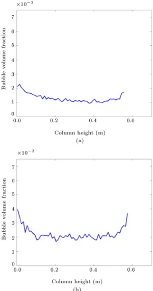
Figure 6 shows average volume fraction of the bubbles along the column height, where Figure 6(a) and (b) represent the time periods from 5-15 s and 16-26 s, respectively. Figure 6(a) and (b) show that the highest bubble volume fraction is located at the bottom of the column. In general, the bubble volume
Figure 6. Average volume fraction of the bubbles along the column height in the gas-liquid-particle three-phase ow in normal gravity: (a) 5-15 s and (b) 16-26 s. (Supercial gas velocity, Us= 0:25 mm/s; initial bubble
size, db= 1:0 mm; and particle size, dp= 0:25 mm.)
fraction decreases along the height of column, attains the minimum at 0.4 m and 0.25 m, respectively, and then increases along the height. The two eects presented below may explain these phenomena. Firstly, as mentioned above, bubble upward velocities along the centerline of the column increase with the height of the column, reaching their maximum values at the heights of about 0.4 m and 0.25 m, respectively, for dierent time durations, while maximum bubble velocities imply the shortest bubble duration time and lowest bubble volume fraction. Secondly, as above mentioned, bubble plume shrinks in the middle of the column and expands at the top of the column due to the liquid vortices. Therefore, bubbles have greater spaces to stay at the bottom and top of the column. Thus, the average volume fraction of the bubbles can be higher in those regions. A comparison of Figure 6(a) and (b) shows that the bubble volume fraction increases with time due to S-shaped bubble plume and separate bubbles. The column contains more bubbles in the late development. Figure 7(a) and (b) show average Sauter mean diameter of the bubbles along the column heights from 5-15 s and 16-25 s, respectively. As seen from Figure 7(a) and 7(b), bubble diameter increases with the column height. The reason is related to bubble-bubble coalescences, which result in the increase of the bubble diameter, and the chance of coalescence is proportional to the bubble duration time; therefore, bubble diameter increases with the column height. A comparison of Figure 7(a) and (b) shows that bubble diameter also increases with the evolution of the ow, because, with the development of the ow, the increase of the bubble upward velocity dierences will result in more bubble-bubble collisions and coalescences. The dramatic increase of the bubble size in the free surface region in Figure 7(a) is due to the rising of free surface. In this region, due to bubble-bubble collisions, bubbles are larger, while there is no smaller bubble to balance those larger bubbles; therefore, the average bubble size is larger.
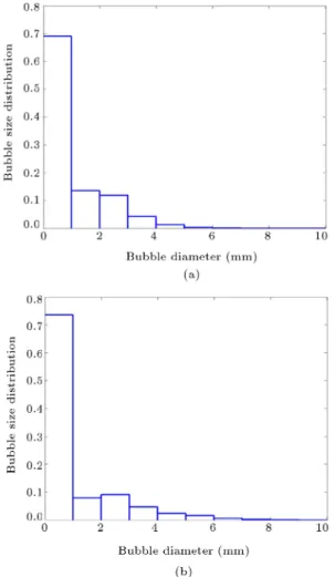
Figure 8(a) and (b) show average bubble size distribution in the entire column from 5-15 s and 16-26 s, respectively. Though the bubble initial diameter is 1 mm, bubbles between 1 and 2 mm own the largest quota due to bubble coalescences. A comparison of Figure 8(a) and (b) shows that, with the evolution of the ow, the quota of small bubbles decreases, and the quota of large bubbles increases due to bubble coalescences.
3.2. Development of transient ow structures in 2 g gravity
To investigate the eect of larger gravity on the phase ow, a study of the characteristics of three-phase gas-liquid-particle ows under 2 g gravity is given in this section. The hydrodynamic parameters
Figure 7. Average Sauter mean diameter of the bubbles along the column height in the gas-liquid-particle three-phase ow in normal gravity: (a) 5-15 s and (b) 16-26 s. (Supercial gas velocity, Us= 0:25 mm/s; initial
bubble size, db= 1:0 mm; and particle size, dp= 0:25
mm.)
used in the simulation are listed in Table 1 (Case 2). Figure 9 shows the snapshots of the liquid stream traces as well as the locations of bubbles and particles at times of 1, 8, 17, and 25 s after the initiation of the ow. Figures 10, 11, and 12, respectively, show the corresponding velocities of bubbles, liquid, and particles. In 2 g gravity, the gravity force for all the three phases as well as the buoyancy force for both particles and bubbles is twice the gravity force in normal gravity condition. Thus, compared to ow with normal gravity, bubbles move faster in the column under 2 g gravity condition.
Similar to the ow with normal gravity, Fig-ures 9(a), 9(b), 10(a), and 10(b) show that bubble plume rises rectilinearly along the centerline of the column; the vortices generated by the pushing of the
Figure 8. Average bubble size distribution of the gas-liquid-particle three-phase ow in normal gravity in the entire column: (a) 5-15 s and (b) 16-26 s. (Supercial gas velocity, Us= 0:25 mm/s; initial bubble size, db= 1:0
mm; and particle size, dp= 0:25 mm.)
Figure 9. Computed ow structure of the gas-liquid-particle three-phase ow in 2 g gravity. (Supercial gas velocity, Us= 0:25 mm/s; initial bubble
size, db= 1:0 mm; and particle size, dp= 0:25 mm.)
plume are almost symmetric at the early development of the ow, as seen in Figure 11(a) and (b). However, with the evolution of the ow, the vortices become non-symmetric as seen in Figure 11(c). Eventually,
Figure 10. Computed snapshots of the bubble velocities of the gas-liquid-particle three-phase ow in 2 g gravity. (Supercial gas velocity, Us= 0:25 mm/s; initial bubble
size, db= 1:0 mm; and particle size, dp= 0:25 mm.)
Figure 11. Computed snapshots of the liquid velocities of the gas-liquid-particle three-phase ow in 2 g gravity. (Supercial gas velocity, Us= 0:25 mm/s; initial bubble
size, db= 1:0 mm; and particle size, dp= 0:25 mm.)
staggered vortical ows are formed, as shown in Figure 11(d), changing the pattern of the bubble plume to S-shape as seen in Figures 9(c), 9(d), 10(c), and 10(d), and the moving of these staggered vortices results in the oscillation of the bubble plume.
Figure 10(b), (c), and (d) show that the bubble upward velocities increase along the column height, attain the maximum at 0.45 m, 0.5 m, and 0.45 m, re-spectively, and then decrease along the column height. The bubble maximum upward velocities as well as the dierences of the bubble upward velocities along the column height increase with time, which may result in more bubble-bubble collisions and coalescences.
Figure 11(b), (c), and (d) and Figure 12(b), (c), and (d) show that the liquid and particle upward velocities increase along the column height. For liquid, all upward velocities attain the maximum at 0.45 m; for particles, the upward velocities attain the maximum at 0.45 m, 0.4 m, and 0.4 m, respectively, and then
Figure 12. Computed snapshots of the particle velocities of the gas-liquid-particle three-phase ow in 2 g gravity. (Supercial gas velocity, Us= 0:25 mm/s; initial bubble
size, db= 1:0 mm; and particle size, dp= 0:25 mm.)
decrease along the column height. These maximum upward velocities and the dierences of these upward velocities along the column height increase with time. Therefore, there are more particle-particle collisions with the development of the ow.
The dierence of location between the maximum upward velocities of bubbles, particles, and liquid indicates that the relaxation eects exist not only at the driving of bubbles to the liquid, but also at the liquid transportation to particles.
A comparison of Figures 9, 11, and 12 indicates that most particles are concentrated outside the large vortices. Figures 11 and 12 show that velocities of particles and liquid are in the same order, and velocities of particle are generally slightly smaller than those of liquid; however, both are much smaller than bubble velocities shown in Figure 10.
Compared with Figure 2(a), Figure 9(a) shows higher bubble plume position, which means that bub-bles under 2 g gravity have larger rising velocities. Besides, compared with Figure 3, Figure 10 shows larger bubble-rising velocities too, which is a result of increasing bubble buoyancy force in the ow under 2 g gravity. Because bubble motions are the source of the three-phase bubbly ow, larger bubble-rising velocities will result in larger liquid and particle velocities, as shown in Figures 11 and 12.
Compared with the rectilinear plume in Fig-ure 2(c), FigFig-ure 9(c) shows that the bubble plume begins to oscillate at 17 s, because of the eect of the non-symmetric liquid vortices as shown in Figure 11(c), while the liquid vortices are still symmetric in Fig-ure 4(c), meaning that, due to the larger bubble-rising velocities, the ow under 2 g gravity develops fast as compared with the ow in normal gravity.
Compared with Figure 3, Figure 10 also shows that there are more bubbles existing in the ow. Since inlet bubble's densities are the same, more bubbles may imply small bubble diameter and low bubble-bubble
co-alescence rate. This could be a result of larger bubble-rising velocities, because larger bubble-bubble-rising velocities imply larger bubble longitudinal distances, which will decrease the bubble-bubble collision and coalescence rate. Besides, larger bubble-rising velocities also imply strong liquid vortices, as shown in Figure 11. As a result, compared with Figure 4, Figure 11 shows larger horizontal liquid velocities at the bottom of the column, which point to the center of the column, and will result in larger relative velocities of bubbles and larger Web numbers when bubbles on the left and right sides collide with each other. Collisions with larger Web numbers mean more bounce-back of the bubbles and less coalescences. Therefore, the diameter of bubbles is smaller, while the number is lager in ow under 2g gravity.
Compared to ow under normal gravity as shown in Figures 2 and 3, there are no separate bubbles seen in Figures 9 and 10. This could be the consequence of larger bubble-rising velocities, too. Because the separate bubbles result from the drag of the liquid vortices, while larger bubble-rising velocities imply larger bubble momentum and inertia, it is relatively dicult for liquid vortices to catch bubbles with large inertia away from a strong bubble plume to become separate bubbles.
Figure 13 shows average volume fractions of the bubbles along the column height under 2 g gravity, where Figure 13(a) and (b) represent the time periods of 5-15 s and 16-26 s, respectively. Similar to the ow under normal gravity, Figure 13(a) and (b) show that the highest bubble volume fraction is located at the bottom of the column, and it decreases along the height of column, attains the minimum at about 0.38 m and 0.2 m, respectively, and then increases along the height. A comparison of Figure 13(a) and (b) shows that the bubble volume fraction increases with time. Compared with Figure 6, Figure 13 shows smaller value due to higher bubble upward velocities under 2 g gravity.
Figure 14(a) and (b) show average Sauter mean diameter of the bubbles along the column height under 2 g gravity, from the time periods of 5-15 s and 16-25 s, respectively. As mentioned above, due to bubble-bubble coalescences, bubble diameter increases with the column height and the evolution of the ow. Compared with Figure 7, Figure 14 shows much smaller value due to less bubble-bubble coalescences under 2 g gravity.
Figure 15(a) and (b) show average bubble size distribution in the entire column under 2 g gravity ow from the time periods of 5-15 s and 16-26 s, respectively. A comparison of Figure 15(a) and (b) shows that with the evolution of the ow, the quota of large bubbles with diameters of 3-7 mm increases due to bubble coalescences, consuming the small bubbles with diameters of 1-3 mm. However, unlike the ow under
Figure 13. Average volume fraction of the bubbles along the column height in the gas-liquid-particle three-phase ow in 2 g gravity: (a) 5-15 s and (b) 16-26 s. (Supercial gas velocity, Us= 0:25 mm/s; initial bubble size, db= 1:0
mm; and particle size, dp= 0:25 mm.)
normal gravity, Figure 15 shows that 1 mm bubbles own the largest quota because of less bubble-bubble coalescences under 2 g gravity. Besides, the quota of 1 mm bubbles increases with the evolution of the ow. The reason is that the developed strong liquid vortices result in larger horizontal liquid velocities at the bottom of the column, as mentioned above, which will result in larger bubble relative velocities for bubble-bubble collisions and less coalescences.
4. Conclusions
Numerical simulations of gas-liquid-solid ows in 1 g and 2 g gravitational conditions were performed using an Eulerian-Lagrangian approach. The two-way cou-pling of bubble-liquid, particle-liquid, particle-particle, and bubble-bubble was included. Bubble coalescences were also included in the model. The transient
charac-Figure 14. Average sauter mean diameter of the bubbles along the column height in the gas-liquid-particle
three-phase ow in 2 g gravity: (a) 5-15 s and (b) 16-26 s. (Supercial gas velocity, Us= 0:25 mm/s; initial bubble
size, db= 1:0 mm; and particle size, dp= 0:25 mm.)
teristics of three-phase ows in dierent gravity rates were studied, and the eects of gravity were discussed. On the basis of the presented results, the following conclusions were drawn:
Because of increased bubble buoyancy in the ow under higher gravity, the three-phase velocities are larger than that of the ow under normal gravity. Therefore, the ow under higher gravity develops fast;
Bubble volume fraction is smaller in the ow with higher gravity due to high bubble velocities;
The Sauter mean diameter of the bubbles with higher gravity shows much smaller value due to less bubble-bubble coalescences;
There are less separate bubbles in the ow with higher gravity due to high inertia of the bubble plume.
Figure 15. Average bubble size distribution of the gas-liquid-particle three-phase ow in 2 g gravity in the entire column: (a) 5-15 s and (b) 16-26 s. (Supercial gas velocity, Us= 0:25 mm/s; initial bubble size, db= 1:0 mm;
and particle size, dp= 0:25 mm.
Acknowledgements
The authors acknowledge the nancial support from the International Doctoral Innovation Centre, Ningbo Education Bureau, Ningbo Science and Technol-ogy Bureau, and the University of Nottingham. This work was also supported by the UK En-gineering and Physical Sciences Research Coun-cil [grant numbers EP/G037345/1 and EP/L016362/1], Ningbo Natural Science Foundation Program [project code 2013A610107], Zhejiang natural science founda-tion [project code LY18E060004], and Ningbo Sci-ence and Technology Bureau Technology Innovation Team [Grant No. 2016B10010].
Nomenclature
CD Drag coecient (dimensionless)
db Bubble diameter (m)
dd Discrete phase diameter (m)
dt Minimum time for next collision (s) fd Coecient used in drag coecient
calculation (dimensionless) Fb Buoyancy force (N)
Fd Drag force (N)
FInt Interaction force (N)
Fl Saman force (N)
Fvm Virtual mass force (N)
G Acceleration due to gravity force (ms 2)
I Unit matrix
md Discrete phase mass (kg)
P Momentum transferred from the discrete phase (Nkg 1)
P Pressure (Nm 2)
Re Fluid phase Reynolds number (dimensionless)
Red Discrete phase Reynolds number
(dimensionless)
ud Fluid phase average velocity (ms 1)
uf Discrete phase velocity (ms 1)
Us Supercial gas velocity
Greek letters
d Phase coecient (dimensionless)
t Time step for liquid phase calculation (s)
"f Liquid phase volume fraction
(dimensionless)
f Liquid bulk viscosity (kgm 1s 1)
f Liquid viscosity (Pas)
d Discrete phase density (kgm 3)
f Liquid phase density (kgm 3)
f Fluid phase viscous stress tensor
(Nm 2)
!f Liquid vorticity (s 1)
References
1. Fan, L.-S., Gas-Liquid-Solid Fluidization Engineering, Butterworths, Boston (1989).
2. Delnoij, E., Kuipers, J.A.M., and Swaaij, W.P.M.V. \Dynamic simulation of gas-solid two-phase ow: ef-fect of column aspect ratio on the ow structure", Chemical Engineering Science, 52, pp. 3759-3772 (1997a).
3. Delnoij, E., Lammers, F.A., Kuipers, J.A.M., and Swaaij, W.P.M.V. \Dynamic simulation of dispersed
gas-solid two-phase ow using a discrete bubble model", Chemical Engineering Science, 52, pp. 1429-1458 (1997b).
4. Lain, S., Broder, D., and Sommerfeld, M. \Experi-mental and numerical studies of the hydrodynamics in a bubble column", Chemical Engineering Science, 54, pp. 4913-4920 (1999).
5. Lain, S., Broder, D., Sommerfeld, M., and Goz, M.F. \Modelling hydrodynamics and turbulence in a bubble column using the Euler-Lagrange procedure", International Journal of Multiphase Flow, 28, pp. 1381-1407 (2002).
6. Lapin, A. and Lubbert, A. \Numerical simulation of the dynamics of two phase gas-liquid ows in bubble columns", Chem. Eng. Sci., 49, pp. 3661-3684 (1994). 7. Besbes, S., Hajem, M.E., Aissia, H.B., Champagne, J.Y., and Jay, J. \Piv measurements and Eulerian-Lagrangian simulations of the unsteady gas-liquid ow in a needle sparger rectangular bubble column", Chemical Engineering Science, 126, pp. 560-57 (2015). 8. Lau, Y.M., Bai, W., Deen, N.G., and Kuipers, J.A.M. \Numerical study of bubble break-up in bub-bly ows using a deterministic Euler-Lagrange frame-work", Chemical Engineering Science, 108(108), pp. 9-22 (2014).
9. Tyagi, P. and Buwa, V.V. \Euler-Lagrange simulations of mono- & poly-dispersed gas-liquid ows in a rectan-gular bubble column", Iscre 23 and Apcre 7 (2014). DOI: 10.13140/RG.2.1.4325.2966
10. Xue, J., Chen, F., Yang, N., and Ge, W. \A study of the soft-sphere model in Eulerian-Lagrangian simulation of gas-liquid ow", International Journal of Chemical Reactor Engineering, 15(1), 20160064 (2016). (Online) 1542-6580, ISSN (Print) 2194-5748, DOI: https://doi.org/10.1515/ijcre-2016-0064
11. Xue, J., Chen, F., Yang, N., and Ge, W. \Eulerian-Lagrangian simulation of bubble coalescence in bubbly ow using the spring-dashpot model", Chinese Journal of Chemical Engineering, 25(3), pp. 249-256 (2016). 12. Masterov, M.V., Baltussen, M.W., and Kuipers,
J.A.M. \Numerical simulation of a square bubble column using detached eddy simulation and Euler-Lagrange approach", International Journal of Multi-phase Flow, 107, pp. 275-288 (2018).
13. Ahmadi, G. \Overview of computational and analyt-ical modeling of particle transport and deposition in turbulent ows", Scientia Iranica, 1, pp. 1-23 (1994). 14. Nikbakht, A., Abouali, O., and Ahmadi, G.
\Nano-particle beam focusing in aerodynamic lenses - an axisymmetric model", Scientia Iranica, 14, pp. 263-272 (2007).
15. Gidaspow, D., Bahary, M., and Jayaswal, U.K. \Hy-drodynamic models for gas-liquid-solid uidization. numerical methods in multiphase ows", FED 185, ASME, New York, NY, pp. 117-124 (1994).
16. Grevskott, S., Sannas, B.H., Dudukovic, M.P., Hjarbo, K.W., and Svendsen, H.F. \Liquid circulation, bubble size distributions, and solids movement in two- and three-phase bubble columns", Chemical Engineering Science, 51, pp. 1703-1713 (1996).
17. Mitra-Majumdar, D., Farouk, B., and Hah, Y.T. \Hydrodynamic modeling of three-phase ows through a vertical column", Chemical Engineering Science, pp. 4485-4497 (1997).
18. Wu, Y. and Gidaspow, D. \Hydrodynamic simulation of methanol synthesis in gas-liquid slurry bubble col-umn reactors", Chemical Engineering Science, 55, pp. 573-587 (2000).
19. Padial, N.T., VanderHeyden, W.B., Rauenzahn, R.M., and Arbo, S.L. \Three-dimensional simulation of a three-phase draft-tube bubble column", Chemical En-gineering Science, 55, pp. 3261-3273 (2000).
20. Gamwo, I.K., Halow, J.S., Gidaspow, D., and Mosto, R. \CFD models for methanol synthesis three-phase reactors: Reactor optimization", Chemical Engineer-ing Science, 93, pp. 103-112 (2003).
21. Li, W. and Zhong, W. \CFD simulation of hydrody-namics of gas-liquid-solid three-phase bubble column", Powder Technology, 286, pp. 766-788 (2015).
22. Bogner, S., Harting, J., and Rude, U. \Direct sim-ulation of liquid-gas-solid ow with a free surface lattice Boltzmann method", International Journal of Computational Fluid Dynamics, 31(10), pp. 463-475 (2018).
23. Zhang, J.P. \Discrete phase simulation of bubble and particle dynamics in gas-liquid-solid uidization systems", Ph.D. Thesis, The Ohio State University (1999).
24. Bourloutski, E. and Sommerfeld, M. \Transient Eu-ler/Lagrange calculations of dense gas-liquid-solid ows in bubble column with consideration of phase in-teraction", Proceedings 10th Workshop on Two-Phase Flow Predictions, Merseburg, pp. 113-123 (2002). 25. Sun, X. and Sakai, M. \Three-dimensional
simula-tion of gas-solid-liquid ows using the DEM-VOF method", Chemical Engineering Science, 134, pp. 531-548 (2015).
26. Zhang, X. and Ahmadi, G. \Eulerian-Lagrangian sim-ulations of liquid-gas-solid ows in three-phase slurry
reactors", Chemical Engineering Science, 60, pp. 5089-5104 (2005).
27. Zhang, X. and Ahmadi, G. \Eects of Particle Den-sity on Gas-Liquid-Solid Flows in Bubble Columns", ASME 2014 4th Joint US-European Fluids Engineering Division Summer Meeting collocated with the ASME 2014 12th International Conference on Nanochannels, Microchannels, and Minichannels, pp.V01CT23A002-V01CT23A002, American Society of Mechanical Engi-neers (2014).
28. Hoomans, B.P.B., Kuipers, J.A.M., and Briels, W.J. \Discrete particle simulation of bubble and slug for-mation in a two-dimensional gas-uidized bed: a hard-sphere approach", Chemical Engineering Science, 51, pp. 99-118 (1996).
29. Harlow, F. and Welch, J. \Numerical calculation of time-dependent viscous incompressible ow of uid with free surface", Physics of Fluids, 8, pp. 2182-2189 (1965).
30. Griebel, M., Dornseifer, T., and Neunhoeer, T. \Numerical simulation in uid dynamics: A practical introduction", The Society for Industrial and Applied Mathematics, Philadelphia, PA (1998).
Biographies
Xinyu Zhang received his BEng, MEng, and Dr Eng Degrees from Energy Engineering at Zhejiang University. He received his PhD in Mechanical En-gineering at Clarkson University. He was a University Post-Doctoral Fellow in Chemical Engineering at the Ohio State University. Currently, he is an Assistant Professor of Mechanical Engineering at the University of Nottingham Ningbo China. His main research interests cover multiphase ows, aerosol dynamics, energy systems, and renewable/clean energy.
Goodarz Ahmadi received his PhD from Purdue Uni-versity and, currently, is a Distinguished Professor and Robert Hill Professor at the Department of Mechanical & Aeronautical Engineering at Clarkson University. His main research interests include multiphase ows, aerosol dynamics, and vibration control.