Bayesian Estimation of Change Point in Phase One Risk Adjusted Control Charts

Bayesian Estimation of Change Point in Phase One Risk Adjusted

Control Charts

Reza Ghasemi

1

*, Yasser Samimi

1

, Hamid Shahriari

1 1

Department of Industrial Engineering, K.N Toosi University of Technology, Tehran, Iran [email protected], [email protected], [email protected]

Abstract

Use of risk adjusted control charts for monitoring patients’ surgical outcomes is now common.These charts are developed based on considering the patient’s pre-operation risks. Change point detection is a crucial problem in statistical process control (SPC).It helpsthe managers toanalyzeroot causes of out-of-control conditions more effectively. Since the control chart signals do not necessarily indicate the real change point of the process, in this researcha Bayesian estimation methodis applied to find the time and the size of a change in patients’ post-surgery death or survival outcome. The process is monitored in phase Iusing Risk Adjusted Log-likelihood Ratio Test (RALRT) chart,in whichthe logistic regression model is applied to take into accountpre-operation individual risks. Markov Chain Monte Carlo method is applied to obtain the posterior distribution of the change pointmodel including time and size of the change in the Bayesian framework and also to obtain the corresponding credible intervals. Performance evaluations of the Bayesian estimator in comparison with the maximum likelihood estimator (MLE) are conducted by means of different simulation studies. When the magnitude of the change is small, simulation results indicate superiority of the Bayesian estimator over MLE, especially when a more accurate estimation of the change point is of interest.

Keywords: Risk Adjusted Control Charts, Change Point, Bayesian Estimation, Markov Chain Monte Carlo (MCMC).

1- Introduction

Risk adjusted control charts which are designed to identify unusual patterns in patients’ after surgery outcomes are used in many clinics and hospitals worldwide. The most frequently-used variables for monitoring purposes are patients’ post-surgery binary and survival time outcomes. Since the patients have different pre-operation conditions in terms of age, gender, hyper tension, etc., which are usually called potential risk factors, there is a need to evaluate individuals ‘risks and adjust patients ‘outcomes, accordingly.

*Corresponding author.

ISSN: 1735-8272, Copyright c 2016 JISE. All rights reserved

Journal of Industrial and Systems Engineering

Vol. 9, No. 2, pp 20-37 Spring (April) 2016

Otherwise, the results of monitoring might be misleading. For monitoring patients’ Bernoulli process of death or survival, or their survival time after surgery, patients’ risk-adjusted outcomes are plotted on an appropriate Risk Adjusted Control Chart (RACC). When the chart signals, it is most likelydueto a significant change in the performance of surgical team.There are many articles in this area, investigating both phases I and II of process control.Most of them have focused on phase II. Unkel et al. (2001) reviewed the statistical methods used for identifying infectious diseases outbreak. Tsui et al.(2010) mentioned Risk Adjusted CUSUM and Risk Adjusted EWMA charts as proper methods for patients’ health surveillance.Cock et al.(2008) reviewed applications of different risk adjusted control charts in monitoring mortality data in clinics. Woodall (2006) provided interesting studies on the use of control charts in public health applications. As one of the most frequently-used control charts,Risk Adjusted CUSUM chart is proposed for monitoring patients’ Bernoulli and survival time data by Collins et al.(2010),Jones and Steiner (2011), Sego et al.(2009), Sibanda and Sibanda (2007), and Steiner et al.(2000). Steiner and Jones (2009) proposed an updating EWMA chart for monitoring patients’ survival time data in which the chart is updated according to time index instead of sample index. Gombay et al. (2011) proposed four truncated and risk adjusted sequential tests for monitoring medical performances. Matheny et al.(2011), Matheny et al.(2007) and Spiegel halter et al. (2003) used Risk Adjusted Sequential Probability Ratio Test (RASPRT) chart for performance analysis in the hospitals and clinics. Alemi and Sullivan (2001) presented a tutorial on risk adjusted X chart and studied its applications inevaluation of diabetes control.

As control charts have a delay on identifying the process changes, the change point analysis is used to find the real time and magnitude of the change. Amiri and Allahyari (2012) have provided a recent review on the estimation methods and their properties for change point identification after an out-of-control signal appears on the monitoring control chart.Woodall and Montgomery (2014) have also recently discussed the capabilities of generalized likelihood ratio (GLR) approach as a generalization of the conventional CUSUM chart for change point detection and diagnosis.

In spite of widespread use of change point analysis in industrial process monitoring, it is rather a new area of research in healthcare quality surveillance. According to Woodall and Montgomery (2014) the application of monitoring in healthcare can be groupedin several categories including aggregation of data, healthcare monitoring, public-health surveillance, and syndromessurveillance. They remark that most focus in health- related issues however, is on the category ofmonitoring in healthcare. Paynabar et al. (2012) used risk adjusted Log-likelihood Ratio Test (RALRT) chart for monitoring patients’ outcomes in phase I and provided MLE estimator of the change point.In addition to patients’ individual risk factors, they included categorical operational covariates such as surgeon groups in their risk adjustment model. Assareh and Mengersen (2012), (2011a,b) and Assareh et al.(2011a,b,c)dealt with finding Bayesian estimators of the timeand the magnitude of the process change in Risk Adjusted CUSUM and EWMA charts in phase II.Despite use of the Bayesianestimation approach inphase II of healthcare process monitoring, there is no use of this approach in phase I. Detecting the change point in phase I however, is quitehelpful asit helps one to detect where the process has changed, find the sequence of in-control data and estimate the in-control process parameters. The flexibility and capability of the Bayesian estimation method is beneficial inconstructing a more realisticmodelin phase I.Therefore in this study we use the Bayesian estimation method for change point detection in phase I patients’ post-surgery Bernoulli outcomes. To be able to compare the performance of the Bayesian estimators with other estimators, the MLE estimators are also obtained in this study, for the data in phase I.Considering Woodall and Montgomery (2014), this study is beneath the category of healthcaremonitoring.

In section 2preliminaries including the risk adjustment and the process change point models areexpressed.In section 3 the process monitoring in phase I is considered.The ML estimations of the time and the size of change are proposed in section 4. In section 5 a Bayesian approach along with the MCMC computational algorithm is proposed to obtainthe Bayesian estimators of the time and the size of the change.In section 6a phase Isurgical outcome dataset is used to examine the control chart’s capability and to obtain a baseline risk adjustment model. The efficiency of the Bayesian estimators are compared with

the ML estimators of the time and thesize on different data sets.Finally, in section 7concluding remarks and potential areas for future researches are proposed.

2- Preliminaries of the problem

2-1- Risk adjustment for binary outcomes

Consider Bernoulli process of patients’ survival or death, which is measured with outcome

, 1, 2,..., ,

i

y i = m where y_i =1 indicates that i th patient dies and y_i =0indicates she/he survives, beyond a 30 days period after surgery. The

m

denotes sample size. The i thpatient’s mortality rate,p_i, is a function of patient’s risks factors as follow:

(

β

, u

),

i i

p =f (1)

Where u_i =(x_i1,..,x_ir),is a vector of patients’ risk factors, β=(

β β

₀, ₁,...,

β

_r)denotes the coefficient vector and f denotes an appropriate link function. Also

r

denotes the number of risk factors. As the outcome is a binary variable the logit function can be used as a reasonable risk adjustment model as follow:

( )

0

1

T

i

1

,

β

u

r i

j

j ij

logit p

β

β

x

=

  = _ _= +

 

∑

(2)

Wherelogit p

( )

_i =log(p_i / (1−p_i)).Hence:

0

0

1

1

exp

. 1 exp

r r

j ij j i

j ij j

x p

x

β

β

β

β

=

=

 

+

 

 

=

  

+ +

  

 

 

 

∑

∑

(3)

Let xi denotes the Parsonnet score which is a composite risk factor. Parsonnet score was also

mentioned in the previous related works such as Sego et al.(2007) and Assarehet al.(2011b). The larger the Parsonnet scorexi,the higher is the death risk of the i thpatient. By considering this composite risk

factorxi,the risk factors and coefficient vectors are summarized as ui =(1, xi)andβ=(

β β

0, 1).So pi

may be obtained as follows:

(

)

(

0 0 11

)

exp 1 exp

i i

i x p

x

β β

β β

+ =

+ + (4)

To obtain the coefficients

β

0and

β

1, the method of maximum likelihood estimation of logistic regression

model proposed by Myers et al. (2002)is applied with the data in section 6.

2-2- The process change point model

To monitor the Bernoulli process of patients’ after surgery death or survival, when the patients possess different pre-operation risks, it is allowed for the in-control process rate to change among patients. Then the observations are checked against the expected rate of death obtained by the risk adjustment model. According to Assarehet al.(2012),“in this setting, a Bernoulli process is in the in-control state when

observations can be statistically expressed by the underlying risk models, taking into account their individualcovariates”. For modeling a change in the process, consider yi,i =1, 2,...,m as independent

phase IBernoulli-distributedobservations. These observations come from patients’ process of death or survival in an interval of 30 days after surgery.The process is initially in-control and each observationy_i

follows a Bernoulli distribution with the failure ratep0i.At an unknown time τ , an assignable cause results in a change in the patients’ failure rate from the in-control p_0ito an out- of-control rate,p_1i, so that

1 0

log

it p

(

_i

)

=

log

it p

(

_i

)

+

δ

,

i

≥

τ

.

(5)

Where

δ

>0represents an increase in patients’ mortality rate. Therefore,

0 0

1

0 0

.

exp( )

/ (1

)

1 exp( )

/ (1

)

i i

i

i i

p

p

p

p

p

δ

δ

−

=

₊

₋

(6)

The change point model is proposed as:

0 1

( )

( )

1, 2,..,

1

,..,

.

i

i i Bernoulli p

Bernoulli p

i

y

i

m

τ

τ

 ∝ 

=

−

=

(7)

3- Phase I process monitoring

By considering equation (7), the phase I control chart is equivalent to testing the following hypothesis:

0 1 0

1 1 0

:

1, 2,...

:

,

1,..,

.

i i

i i

H

p

p

i

m

H

p

p

i

τ τ

m

  

=

=

≠

=

+

(8)

To monitor the process in phase I, RALRT chart which is constructed based on the observations’ likelihood function and the change point model is applied. By considering hypothesis (8), underH₀, according to Paynabar et al. (2012)the corresponding log-likelihood function is written as

(

)

( )

(

)

(

)

( )

0 0

1 i=1 0 0

0 0

i=1

.

log |

log

1

log 1

log(1

)

m

i i i

m

i i i i

m

i i i

L P y p

y

p

y

p

y logit p

p

=

  _{ }

  _{ }

  _{ }

 

 

 

 

= =

+ −

−

+

−

=

∏

∑

∑

) 9 (

Under alternative hypothesis the log-likelihood function is written as

(

)

(

)

1

1 0 1

1

( )

log

|

log

|

m

i i i i

i i

L

P y p

P y p

τ

τ

τ

−

= =

   

   

 

 

=

∏

+

∏

( )

{

}

{

( )

}

1

0 0 1 1

i=1 i=τ

,

log(1

)

log(1

)

,

1,...,

.

m

i i i i i i

y logit p

p

y logit p

p

l l

m

l

τ

τ

−

=

+

−

+

+

−

=

+

−

In equations (9) and (10) the process failure rates,p_0i,and p_1iare unknown and need to be estimated. For estimating the failure rates underH₀,p₀i, (i =1, 2,...,m,), all patients’ risk data are considered as a

homogeneous dataset. Hence, the MLE method proposed by Myers et al.(2002)may be used to estimate the coefficient vector of the risk adjustment model. The

β

ˆ₍T_1,m) =(

β

ˆ_0,(1,m),

β

ˆ_{1,( ,1m)})

denotes the ML estimator of the risk adjustment modelparameters.The ML estimator of the failure rates

0i for 1, 2,...,

p i = munder H₀are denoted bypˆ_0i(1,m),which can be obtained by substituting

β

ˆ_{(1, )}T_m in equation (4).UnderH₁the observations are divided at a potential change point.Whena change occurs at the unknown time ,τ the data before and after the change point are not homogeneous. In this situationthe risk adjustment model coefficients are estimatedseparately before and after the process change. Consider

0,(1, 1) 1,( , )

) 1 1

(1, 1

ˆT ₍ˆ _, ˆ ₎

τ τ

τ

β

β

β

− = − − and ˆ( , ) (ˆ0,( , ), ˆ1,( , ))

T

m m

m

τ

β

τ

β

τ

β

= as the ML estimators of the risk adjustment model parameters corresponding to observations 1 to

τ

−1 and τ tom , respectively, underH₁. The coefficients can be obtained using the iterative method proposed by Myers et al.(2002).Hence, the ML estimators of p0i for i =1, 2,...,

τ

−1 and p1i for i =

τ τ

, +1,...,munder the H1, are pˆ0 (1,′i τ −1) and

1 ( , )

ˆ_{i m}

p _τ respectively. These estimators are obtained by substituting

β

ˆ₍₁T_,τ−1) and

β

ˆ₍T_τ,m) in equation (4).As Hogg and Craig(2004)proposed, in the LRT method, the chart’s statistic is the ratio of the data likelihood function under hypotheses H₁and H₀. Since in this paper the data log-likelihood function isused, the ratio of the likelihood functions is changed to their logarithm subtraction. Therefore, considering the log-likelihood functions in equations (9) and (10), RALRT chart’s statistic could be obtained asthe following equation:

1 0

( )

τ

L ( )

τ

L ,

τ

l l, 1,...,m l.

Λ = − = + − (11)

It is assumed that

τ

=l l, +1,...,m −l, wherelis the minimum sample size required to estimate the coefficients of the risk adjustment model.

4- ML estimation of the change pointparameters

Λ( )

τ

s are plotted against time index τ and as long asΛ( )

τ

s are under a pre-specified upper control limit, UCL, the process is considered in control, otherwise it is in out-of-control status. In this situation, the ML estimator of the change point is the time when the likelihood function receives its maximum value. Therefore, according to Paynabar et al.(2012):

( )

mle

, 1,.,

{

max

(

Λ τ

ˆ

)}.

l l m l

arg

τ

τ

=

_{= + −} (12)

Substituting the patients’ modified mortality rates pi1 for i =

τ τ

, +1,...,mfrom equation (6) and

replacing τ by its corresponding value,

τ

ˆ_mle, from equation (12), into equation (10), the log-likelihood function changes to:

( )

{

}

1

1 0 0

0 0 0 0 ˆ i=1 ˆ exp( )

log 1 .

1 ( , )

log

1

log(1

)

mle mle i i i i i i i i m i p p

p

p

p

y

p

L

y logit

τ τ

τ

δ

δ

δ

− =      − +  _ _    _{ } _{ − }    

+

−

 

=

∑

+

−

+

∑

(13)

The ML estimator of

δ

is the value that maximizes equation (13).The partial derivative of equation (13) with respect to

δ

is

1 0 0 0 ( , )

.

ˆ

exp( )

1

exp( )

mle i i i i L

m

i

y

p

p

p

τ δ

δ

_τ

δ

δ

  ∂    

∂

=

₌

∑

_

−

−

+

_ (14)

Sincesetting this differential equation equal to zero results in no closed form solution for

δ

,the Newton-Raphson’s numerical method is applied to solve the equation for

δ

. “This method is based on the derivative of a given equation with respect to its unknown parameters that uses the following linear approximationequation”(Perry et al, 2006):

(

)

( )

d

( )

,

f x

x

f x

f x

x

dx

+ ∆ ≈

+

∆

(15)

where ∆ =x x_k −x_k−1. Whenf x( + ∆x)is set to zero and the equationis rearranged then

(

)

(

1

)

1 ' 1

,

k k k k

f x

x

x

f

x

− − −

=

−

(16)

wherex_kis the value of

x

at the kthiteration of the algorithm. Using an initial value and an termination threshold, this method will converge to the optimum value of f x( ). Using this method to solve equation (14) for

δ

results in:

1 1 1 1 1 0 0 0 1 2 0 2 0 0 ˆ ˆ . ( exp( )

1 exp( )

1 ) exp( )(1 exp( ))

(1 exp( ))

k k k k k i i i k k

i oi oi

i i i i i m m p p p

P P P

P P y τ τ

δ

δ

δ

δ

δ

δ δ

− − − − − − = =         _{− + −}     − + _ + − 

=

−

−

−

∑

∑

) 17 (

The algorithm ends when the |

δ

_k −

δ

_k−1|is smaller than a pre specified partial positive constantε.In this paper the initial value

δ

₀ and the ending measureε are set to 0and10−4, respectively. The algorithm converges to

δ

ˆ_mle , the MLE estimator of the shift size after finite iterations.

5- Bayesian estimation

5-1- Priors

“Statistical inferences for a quantity of interest in a Bayesian framework are described as the modification of the uncertainty about their value in the light of evidence, and Bayes’ theorem precisely specifies how this modification should be made as below” Assareh et al.(2011b):

.

posterior

∝

likelihood

×

prior

(18) The word “Prior” indicates the knowledge about the quantity of interest in terms of a probability distribution before any observation is made.The word “Likelihood”notifies the underlying likelihood function of the observations, and the word “Posterior” is the state of knowledge about the quantity after the data is observed. This is also a probability distribution.

In this section the Bayesian estimators of change point parameters,τ and

δ

are proposed. The first step is to determine the appropriate prior distributions for τ and

δ

. Assareh et al.(2011a,b)suggested the use ofuniform and truncated normal distributions as the prior distributions for the time and the size of the change point, respectively. However, since

δ

is assumed to be a positive quantity, it is possible to use other positive distributions such as gamma.

Here the uniform distribution u l m( , −l) is applied as a prior for the change time τ because it is assumed that a change can occur at any time in the interval( ,l m −1).For the change magnitude however, the gamma distributionsG a b( , ) is considered. The values ofa and bare chosen in such a waythat reflect the prior knowledge about the change magnitude. Here a realistic and practical assumption is considered. It is assumed that when a change occurs in the process due to surgical team performance, it cannot be a fundamental change that radically increases the mortality rates. The reason for this assumption is that the surgical team is professional however, and has gained some experiences still.Therefore the values for a and b are set to 2 and 0.5 that result in a prior density function that is denser in the interval [0, 2] having a mean equal to 1. Consequently, the probability for a large

δ

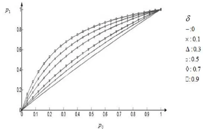
is small. The effect of different change sizes in the in-control rate p0,according to the equation (6), is displayed on

Figure 1.

Considering the priors:

1

1 1

( ) ,

(m l) ( )l m 2l

π τ

= =

− − −

1 2

exp( )

( ) ,

( )

a

a b a b

δ

δ

π δ

= − −

Γ

) 19 (

The likelihood function is

(

)

(

)

1

0 1

1

0 0 1 1

1 1

1 1

.

|

|

(1

)

(1

)

i i i i

m

i i i i

i i

i i i i

y y m y y

i i

L

P y p

P y p

p

p

p

p

τ

τ τ

τ

−

= =

− −

−

= =

=

−

=

×

−

∏

∏

∏

∏

(20)

0 0

0 0

0 0

1

1 1

/ (1

)]

(1

)

/

[exp( )

.

1

exp( )

(1

)

i

i i

y

y i

i i

i i

y i

m

i i

p

p

L

p

p

p

p

τ

τ

δ

δ

− −

= =

−

−

−

=

+

∏

∏

(21)

Considering the equation (18), the joint posterior distribution may be expressed as

1 2

( , |y) L ( ) ( ).

π τ δ

∝ ×

π τ π δ

× (22)

By simplification and omitting the irrelevant parameters the joint posterior distribution would be

(

0

)

1

0 0

0

0 0

1 1

1 / (1 )]

( , | ) (1 [exp( )

1 exp(

) exp( ).

/ 1

) ( )

i

i i

i i

y a

i i

i i

m

i i

y y p

y p p

p b

p

p τ

τ

π

δ

τ δ

−

δ

δ

−

δ

= =

−  

 

+

−

∝ − −

−

 

∏

∏

(23)

As the joint posterior distribution has no specific form, it is difficult to obtain the posterior distribution for each parameter. Therefore, in the next section the Markov Chain Monte Carlo(MCMC ) simulation method is employed to obtain posterior distribution forthe unknown time and the size of the change, τ and

δ

.

5-2- Markov Chain Monte Carlo (MCMC) Simulation

MCMC approach includes methods to sample from univariate and multivariate distributions in which the samples constitute a Markov chain. Gibbs sampling and Metropolis-Hasting (M-H) methods are quite popular in the context of MCMC approach. Sometimes it is impossible to directly sample from the conditional posterior distribution of the parameters.In these cases using MCMC methods to obtain the posterior distributions is very helpful. Although the Gibbs sampling is aneffective technique to generate samples from the conditional distributions of two or more variables, it fails to work with highly complicated multivariable distributions as it requires decomposition of the joint posterior distribution into full conditional distributions. In this paper, the M-H algorithm is applied to obtain the posterior distributions of the change point parameters. The key advantage ofM-H algorithm is itsefficiencyto work with multivariate distributions. For more details on MCMC methods readers are referred to Fienberg et al.(2007) and Colosimo and Castillo(2007).

5-3- M-H algorithm for estimating change point parameters

Considering the joint posterior distribution of τ and

δ

in equation (23),the conditional distribution for each parameter can be obtained as follows:

(

)

0 0

0 0

0 0

1

1 1

[ / (1

exp( )]

( | , ) (1 )

/ ( ) ),

1 exp( ) (1 )

i

i i

i i

i y

i

i i

m

i i

y y

y p p p p m

p p

τ

τ

π

δ

τ δ

δ

τ

−

=

− =

−

∝ −

−

 

−

 

+

 

∏

∏

(24)

(

)

1

0

1 0

( | , ) 1 exp( ) _i / (1 _i) a exp(( 1/ ) ).

m

i

p p m b

y

τ

π δ

τ

δ

−

δ

₋

τ

δ

= − −

∝

∏

+ − (25)

Although these conditional distributions have unknown forms, the graphical assessmentof them shows that they may be approximated bythe Normal and the Weibull distributions, respectively. To execute the M-H algorithm, the first step is to choose a proposal density function for each parameter. Here the normal distribution N(τ(k−1), )λ and the Weibull distribution W bl v( ₁δ(k−1),v₂)are chosen as the proposal distributions ofτ and

δ

, respectively.τ(k−1)andδ(k−1) are the values of τ and

δ

in (k −1)st iteration of the algorithm and

λ

=1,v₁=1.5,andv₂=2.5are set to the stated parameters. As the values of the likelihood function and the conditional distributions are too small, their logarithms are usedinstead of the algorithm. The algorithmfor obtaining marginal posterior distributions is as follows:

Algorithm for obtaining posterior distributions of τ and

δ

1. Start with initial value

τ

(0) and

δ

(0). 2. Set k=1,

3. Use M-H algorithm, generate

τ

( )k from posterior

π τ

( (k−1) |y,

δ

(k−1)) with proposed normal distribution N(τ(k−1), )λ .

4. Use M-H algorithm, generate

δ

( )k from posterior

π δ

( (k−1)| ,y

τ

(k))with proposed Weibull distributionW bl v( ₁δ(k−1),v₂).

5. Set k = +k 1.

6. Repeat steps3-5, N times.

The algorithm converges in finite steps. Good starting values will accelerate convergence. N is set to 10000and the first 25% of the samples are considered as burn-in values and removed as they come from unstable posterior distributions of τ and

δ

. So the last 75% samples are used to obtain the Bayesian

estimators. Having the posterior distributions, the mean and the median of each distribution,

τ τ

,%and ,

δ δ% _{, are used as Bayesian estimators for the time and the size of the process change.}

6- Discussion

6-1- An application in phase I cardiac surgery data

A data set containing the patients’ cardiac surgery data whichwas considered by different authors including Sego et al. (2009) and Paynabar et al.(2012) is examined here.The Patients’ potential risk data are represented by their Parsonnet scores. Sego et al. (2009) stated that the Parsonnet scores are closely approximated by an exponential distribution with mean 8.9. Paynabar et al.(2012) considered the first two years data(including data for m=1000 patients) as the phase I data for estimating the risk adjustment model parameters and obtained[

β β

ˆ₀, ˆ₁] [ 3.373, 0.073]= − . Therefore,

( )

exp( 3.473 0.073 )

3.473 0.073 .

1 exp( 3.473 0.073 ˆ

)

ˆ i

i i i

i

x

logit p x p

x

− +

= − + ⇒ ₌

+ − + (26)

In this study the data for phase I are generated by means of simulation using the risk adjustment model in equation (26).Theupper control limit of the RALRT chart of Paynabar et al.(2012) is also applied here. They obtained the simulated UCL’s for different sample sizes (

m

), different numbers of the risk adjustment model coefficients( )

β

and two different values of the type I error probability,α,as 0.05 and 0.01.The number of patients and the number of the risk adjustment model coefficients in this simulation study are m =1000 and 2, respectively. For

α

=0.01,the UCL is considered to be 6.48. The value for

l, the minimum sample size , is set to 5 in the numerical examples. Also on the basis of some trial and error, the values of a and b, the parameters for the prior distribution of

δ

are set to 2 and 0.5, respectively. The Parsonnet scoresx_i, for i =1, 2,...,1000, are generated from an exponential distribution with mean equal to 8.9 as the patients’ risk scores. Substituting for x_i,i =1, 2,...,1000 in equation (26),the mortality probabilities,pi ,i =1, 2,...,m are obtained for the m=1000 patients.

Then, Bernoulli outcomes y_i ,i =1, 2,...,m are independently generated from the Bernoulli distributions with the failure rates,p_i, fori =1, 2,...,1000as the patients’ after surgery death or survival outcome. Finally,these data are considered as the phase I dataset and the RALRT control chart is used to evaluate them. The chart is displayed in Figure 2. Investigation of Figure 2 reveals that all the values are under the UCL. So the process is inits control state. Therefore, the risk adjustment model in equation (26) may be applied as a base risk-adjustment model to monitor observations during phase II.

Figure2. The RALRT chart for the phase one data

6-2- Performance Evaluation of Bayesian Estimators

In this section simulated data aregenerated to examine the Bayesian estimators’performancein detecting the time and the size of the process change. The risk-adjustment model given in equation (26) is used to generate data. Following steps areexecuted to simulate data and thento obtain the estimates.

1- One thousand Parsonnet scoresx_i ,i =1, 2,...,1000 are generated from an exponential distribution with mean equal to 8.9. Then by substituting them into equation (26), the values for patients’ initial risk,p_0i, i =1, 2,...,1000are obtained.

2- Using equation (6), a shift equal to

δ

at time τ is considered and the values for

1i, , 1,...,

p i =

τ τ

+ m

are obtained. Then, the patients’ Bernoulli outcomes yi,i =1, 2,...,1000

are produced independently from the patients’specific Bernoulli distributions using the rates equal to p0i,i =1, 2,...,

τ

−1 _{for patients 1 to}τ −1_{, and the rates equal to} p1i, i =

τ τ

, +1,...,m

for patients τ to

m

.

The simulated Bernoulli data and the corresponding risk factors are regarded as phase I data and the RALRT chart with the UCL= 6.48 is applied to monitor the mortality rate.

3- When the chart signals, the MCMC simulation is performed and the values for Bayesian estimates of the time and the size of the change areobtained.

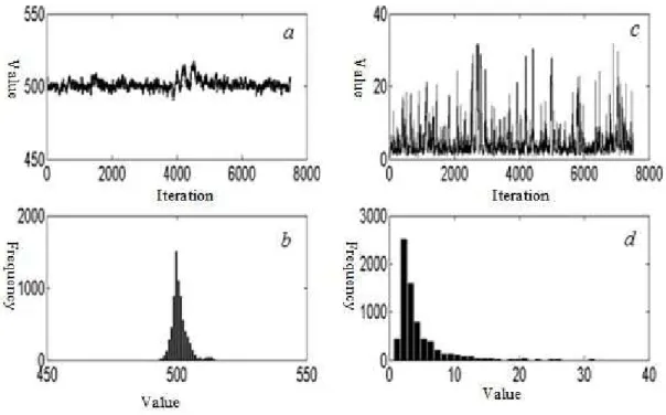
The MCMC output and the posterior distribution of τ and

δ

when the real change point and change size are 500 and3 respectively, are shown in Figure3. Table 1 shows Bayesian estimates and the standard deviation for the posterior distributions of τ and

δ

for the values of τ and

δ

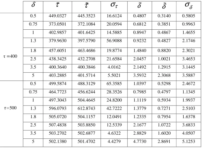
equal to(400, 500), and

(0.5, 0.75, 1, 1.3, 1.8, 2, 5, 3.5, 5), respectively. Comparing the Bayesian estimates of the change time for

τ

=500 indicate that for

δ

smaller than 1.3 the posterior mean

τ

provides more accurate estimates of τ than the posterior median

τ

% and for

δ

greater than 1.3 the

τ

% is a better estimator of τ . When

500

τ

= , the values obtained for

τ

and

τ

%, are more accurate than those obtained for

τ

=400.For the change size, when

τ

=500, the posterior median

δ

% is more appropriate than the posterior mean

δ

for

0.5.

δ

= However, when

δ

>0.5

for all

δ

’s,

δ

outperforms

δ

%

.

As in the Bayesian framework the posterior distribution for each parameter is

intervals maybe obtained. “A credible interval is a posterior probability based interval which involves those values of the highest probability in the posterior density of the parameter of

2012). Similar to Assareh et al. process change are considered and

of the 50% and the 80% credible intervals of reveals that the posterior distribution of the change increase in the probability. In other words

472.4215 to428.5558 in comparison to This interpretation may be extended to

Figure 3. MCMC output and posterior distributions of

, :

a c

MCMC output of

0.5,

δ

estimates the change size more precisely than As in the Bayesian framework the posterior distribution for each parameter is

obtained. “A credible interval is a posterior probability based interval which involves those values of the highest probability in the posterior density of the parameter of

(2011b), the 50% and the 80% of the estimated time and process change are considered and are shown in Table 2 for

τ

=

(400, 500)

and

80% credible intervals of the estimated time of the change

posterior distribution of the change time is more skewed to the left with In other words an increase in the probability changes

in comparison to the right boundary which increases from 502.8745 to 507.7336. be extended to the other situations of change point and change size.

MCMC output and posterior distributions of τ and

δ

for

τ

=500

MCMC output of τ and

δ

b d

, :

posterior distributions of τ

than

δ

% . When

τ

=400 As in the Bayesian framework the posterior distribution for each parameter is accessible, the credible

obtained. “A credible interval is a posterior probability based interval which involves those values of the highest probability in the posterior density of the parameter of interest”(Assaeh et al. 0% of the estimated time and the size of the

(0.5,1)

δ

=

.Comparison

of the change for

τ

=500 and

δ

=1

is more skewed to the left with respect to the changes the leftboundary from right boundary which increases from 502.8745 to 507.7336. other situations of change point and change size.

500 and

δ

=3.

Table 1. Bayesian estimation of change point parameters

δ

σ

δ

%

δ

τ

σ

τ

%

τ

δ

0.5805 0.3140 0.4807 16.6124 445.3523 449.0327 0.5

τ=400

0.9963 0.3851 0.6812 20.0594 372.1084 373.0501 0.75 1.4655 0.4867 0.8947 14.5885 401.6425 402.9857 1 2.1746 0.4827 0.9232 56.9088 397.5790 379.9630 1.3 2.3021 0.8820 1.4840 19.8774 463.4686 457.6051 1.8 3.4653 1.0021 2.0457 21.6584 432.2708 438.3425 2.5 3.1445 1.2915 2.1492 4.0162 400.3846 400.3640 3.5 3.5887 2.3068 3.5932 5.5021 401.5714 403.2885 5 2.4672 0.5298 1.0397 65.3585 488.3129 499.5874 0.5 =500 1.1345 0.4797 0.7985 28.3526 456.6244 464.7723 0.75 1.9937 0.5934 1.1119 24.8200 504.4645 497.3043 1 2.5103 0.7271 1.3779 42.7222 612.8743 596.0793 1.3 1.6378 0.7954 1.2335 12.0491 504.1157 505.0720 1.8 3.6833 1.0722 2.1677 12.5339 503.8850 507.4838 2.5 4.0507 1.6020 2.8829 4.6322 502.6877 503.2702 3.5 5.1253 2.8691 4.7730 4.4279 501.4702 502.1380 5

Table2. Credible Intervals for Change point parameters

80 % 50

% Parameter

δ

τ

[346.7161 475.3345] [361.2815 452.3534]

τ

0.5

400

[0.2061 1.8691] [0.2979 0.8764]

δ

[281.4053 419.2256] [312.7669 400.4298]

τ

1

[0.1156 1.1197] [0.1907 0.5841]

δ

[454.9908 511.9533] [467.4823 504.2285]

τ

0.5

500

[0.1977 1.6794] [0.3033 0.8755]

δ

[428.5558 507.7336] [472.4215 502.8745]

τ

1

[0.2736 2.0942] [0.3852 1.0493]

δ

6-3- Comparison of the Bayesian estimators with the MLE estimators

Studying the performance of the proposed Bayesian estimators, 100 datasets are generated usingthe steps 1 and 2 in section 6-2. The Bayesian estimators and the maximum likelihood estimators of the change point parameters are obtained for each set of data. Then the mean and the standard deviation of the estimators are computed. Table 3 shows the resulted mean and standard deviation for each estimator. Concerning this table, the Bayesian estimators

τ

and

τ

% outperform the MLE estimator

τ

ˆ_mlefor both small and large shifts. In addition, the standard deviation of

τ

%is much smaller than

τ

ˆ_mle. As an example, for

τ

=500 and

δ

=0.7781,we have

τ

=503.1559,

τ

% =502.711 and

τ

ˆ_mle =492.0625. The corresponding standard deviations areSD( )

τ

=58.7352, SD( )

τ

% =62.4293 and

ˆ

( _mle) 127.4563

SD

τ

= .Comparison of

τ

and

τ

%shows that they perform almost the same. On the other hand, regarding the change size estimators, for

δ

≤1, in two cases the Bayesian estimator

δ

% and in four cases the MLE estimator

δ

ˆ_mle are the most accurate ones. However, for

δ

≥1 in two cases

δ

% and in two other cases

δ

ˆ_mleproduce more precise estimates of the change size.

The credible intervals are also given to evaluate the performances of the estimators. The credible intervals

3 4 lt s sh o w t h at f o r th e ch an g e ti m e es ti m at o rs , in c o m p ar is o n t o

ˆmle

τ

,i n m an y s im u la ti o n r u n s th e

τ

an d e w it h in t h e sp ec if ie d i n te rv al s ar o u n d

τ

. F

o r in st an ce , th e p ro b ab il it y o f

τ

a n d ˆ

τ

bei

n g w it h in ± 1 0 o f 5 0 0 w h en 0 .5

δ

= ,i s 0 .2 1 4 3 a n d 0 .1 4 2 9 ,r es p ec ti v el y . W h il e fo r

ˆmle

τ

th e p ro b ab il it y i s eq u al t o 0 i n as e. F o r 1

δ

< th e ch an g e si ze e st im at o r

δ

% s

u rp as se s th e es ti m at o rs

δ

an d

ˆ mle

δ

. W h il e fo r 1

δ

≥ e is n o s u p er io r es ti m at o r.

Table 3.Comparison of Bayesian and MLE estimators for = 500 and a range of

0.2041 0.4771 0.5 0.6021 0.7781 1 2 3 5 7.5 10 456.9022 479.8635 495.2615 509.7522 503.1559 530.8575 552.1965 525.0353 503.5180 501.4740 501.1294 458.8763 481.6228 492.8620 507.0434 502.7110 531.9220 552.9419 524.6791 502.6352 500.8396 500.5755 511.1110 505.7910 595.5000 520.3617 492.0625 526.6393 495.2490 494.6101 489.2500 494.8401 551.3294 72.2927 76.7997 47.6041 61.9235 58.7352 44.9611 32.7508 25.8160 3.4221 0.8976 0.4268 73.0659 80.1885 49.0743 65.8224 62.4293 50.5956 35.5530 28.3498 3.4769 0.8926 0.3792 328.4438 253.1331 267.7504 186.1663 127.4563 118.0719 10.1684 7.9302 30.8739 1.6558 15.3051 0.6584 0.8628 1.1130 0.8958 0.9296 1.338523 1.8038 2.4668 5.3356 10.0104 13.1989 0.3664 0.4467 0.6237 0.4952 0.5105 0.7334 0.9857 1.3921 3.3032 7.0350 10.0820

7- Conclusion

In this study the Bayesian estimators of the change point parameters (including time and size of the change) are proposed forphase I analysis of the patients’ post-surgery death or survival risk-adjusted outcomes. In the Bayesian estimation, for eachτ and

δ

two Bayesian estimators including the mean and the median of the corresponding posterior distribution are proposed. Having the whole posterior distribution of the parameters in the Bayesian framework is a remarkable advantagethat enabled us to construct credible intervals for unknownτ and

δ

. Results show that in comparison to MLE, Bayesian estimation method effectively detects the true change point parameters. In the simulation study, the Bayesian method significantly outperformed MLE when the change time is estimated.

In this approach the prior distributions of the change point parameters (time and size) have been considered to be independent.In practice, however, there are situations in which this assumption may not be valid.As an example,over the night working hours, due to the physicians’ fatigue when a change occurs it may be more severe than the same change during the daytime. In such cases it is more reasonable to consider dependencybetween the parameters and,as a result, use a joint prior distribution to describe their behaviors.

In this paper, it was assumed that after a change occurs, the process remains in the new state as long as no out-of-control signal appears on the control chart. While, in practice as the surgeon’s or physician’s proficiency increases the process improves. Considering this assumptionmay lead to a more realistic model. Hence, another potential area for future research may be considering the incorporation of physicians’ learning process into the model.

Table4: Estimated precision performance over

τ

=500 and a given range of

δ

. (continue)

0.6200 0.3200

0.100

δ

0.9400

0.7800

0.3800

τ

5

_τ

_%

_0.5400

_0.8400

_0.9600

_δ

_%

_{0 0 0.0100}

0.9700 0.9700

0.1200

ˆ MLE

δ

0.9300

0.7600

0.0200

ˆ

_MLE

τ

0 0

0

δ

1

1

0.8600

τ

7.5

τ

_%

0.9300

0.9900

₁

_δ

%

0.0800 0.1400 0.3000

0.9300 0.0200

0.0200

ˆ MLE

δ

1

0.7100

0.0100

ˆ

_MLE

τ

0 0

0

δ

1

1

0.9900

τ

10

τ

%

1

1

1

_δ

%

0.0800 0.1400 0.3100

0 0

0

ˆ MLE

δ

1

0.6700

0.0300

ˆ

_MLE

References

Alemi, F. and Sullivan,T. (2001).Tutorial on Risk Adjusted X-Bar Chart: Application to Measurement of Diabetes Control. Quality Management in Healthcare, 9, 57-63.

Amiri, A., &Allahyari, S. (2012). Change Point Estimation Methods for Control Chart

PostsignalDiagnostics: ALiteratureReview. Quality and Reliability Engineering International, 28(7), 673-685.

Assareh, H . Smith, I. and Mengersen, K. (2011a). Bayesian Estimation of the Time of a Linear Trend in Risk Adjusted Control Charts. IAENG International Journal of Computer Science, 38, 409-417.

Assareh, H . Smith, I. and Mengersen, K. (2011b). Bayesian Change Point Detection in Monitoring Cardiac Surgery Outcomes .Quality Management In Healthcare, 20, 207-222.

Assareh, H . Smith, I.andMengersen, K. (2011c). Change Point Detection in Risk Adjusted Control Charts. Statistical Methods in Medical Research, 0, 1-22.

Assareh, H. and Mengersen, K. (2011b). Bayesian Estimation of the Time of a Decrease in Risk Adjusted Survival Time Control Charts. International Journal of Applied Mathematics, 41, 360-366.

Assareh, H. and Mengersen, K. (2012). Change Point Estimation in Monitoring Survival Time. PLoS

ONE. 7,1-7.

Assareh, H. and Mengersen, K.(2011a). Detection of the Time of a Step Change in Monitoring Survival Time.Proceedings of the World Congress on Engineering, London, U.K. July 6-8, 1: 1-9.

Collins, G. S .Jibawi, A. and McCulloch, P. (2010). Control Chart Methods for Monitoring Surgical Performance: A Case Study from Gastro-Oesophageal Surgery. Journal of Cancer Surgery (EJSO). 37, 473-480.

Colosimo, B.M. Castillo, E.D. Editors.(2007). Bayesian Process Monitoring, Control and

Optimization.US.CRC Press.47-66.

Cook, A.D. Duke, G. Hart, G.K. Pilcher, D. and Mullany, D. (2008). Review of the Application of Risk-Adjusted Charts to Analyse Mortality Outcomes in Critical Care.Critical Care Resuscitation. 10,239-251. Fienberg, S.E. van der Linden, W.J. Editors. Lynch, S.M. (2007). Statistical for Social and Behavioral

Science. Section11: Introduction to Applied Bayesian Statistics and Estimation for Social Scientists.

USA.Springer Science+ Business Media.105-150.

Gombay, E. Hussein, A.A. and Steiner, S.H.(2011). Monitoring Binary Outcomes Using Risk-Adjusted Charts: a Comparative Study.StatisticsIn Medicine. 30, 2815-2826.

Hogg, R.V. Craig, A.T. (2004). Introduction to Mathematical Statistics.Pearson Education. China. 413-420.

Jones, M.A. and Steiner, S.H. (2011).Assessing the Effect of Estimation Error on Risk-Adjusted CUSUM Chart Performance.International Journal for Quality in Healthcare.24, 1-6.

Matheny, M.E. Machado, L.O. and Resnic, F.S. (2007).Risk-Adjusted Sequential Probability Ratio Test Control Chart Methods for Monitoring Operator and Institutional Mortality Rates in Interventional Cardiology.American Heart Journal. 155, 114-120.

Matheny, M.E. Normand, S.L.T. Gross, T.P. Dabic, D.M. Berrios, N.L. Vidi,V.D. Donnely, S. and Resnic, F.S. (2011).Evaluation of an Automated Safety Surveillance System Using Risk-Adjusted Sequential Probability Ratio Testing. BMC Medical Informatics and Decision Making. 11,1-8.

Myers, R.H. Montgomery, D.C. Vining, G.G.(2002). Generalized Linear Models.John Wiley & Sons, Inc. New York. 322-328.

Paynabar, K. and Jin, J. (2012).Phase I Risk-Adjusted Control Charts for Monitoring Surgical Performance by Considering Categorical Covariates. Journal of Quality Technology. 44, 39-53. Perry, M.B. PignatielloJr, J.J. Simpson, J.R. (2006). Estimating the Change Point of a Poisson Rate Parameter with a Linear Trend Disturbance.Quality and Reliability Engineering International.22,371-384. DOI: 10.1002/qre.715.

Sego, L.H. Marion, R. Reynolds, Jr. Woodall, W. (2009).Risk-Adjusted Monitoring of Survival Times.StatisticsIn Medicine. 28, 1386-1401.

Sibaanda, T. and Sibanda ,N. (2007). The CUSUM Chart Method as a Tool for Continuous Monitoring of Clinical Outcomes Using Routinely Collected Data. BMC Medical Research Methodology.7, 1-7.

Spiegelhalter, D., Grigg, O., Kinsman, R. and Treasure, T. (2003).Risk-Adjusted Sequential Probability Test. applications to Bristol, Shipman and adult cardiac surgery.International Journal for Quality in

Health Care.15, 7-13.

Steiner, S.T. and Jones, M. (2009). Risk-Adjusted Survival Time Monitoring with an Updating

Exponentially Weighted Moving Average (EWMA) Control Chart. Statistics In Medicine. 29, 444-454. Steiner, S.T. Cook, R.J. Farewell, V.T. and Treasure, T. (2000).Monitoring Surgical Performance Using Risk-Adjusted Cumulative Sun Charts.Biostatistics. 1, 441-452.

Tsui, K.L. Goldsman, D. Jiang, W. and Wong, S.Y. (2010).Recent Research in Public Health Surveillance and Health Management.Prognostics& System Health Management Conference.Macau.MU 3059. 0,1-22. Unkel, S. Farrington, P. Garthwaite. P.H. Robertson, C.and Andrews, N. (2011). Statistical Methods for the Prospective Detection of Infectious Disease Outbreaks: A review. Journal of the Royal Statistical

Society: Series A (Statistics in Society). 175, 49-82.

Woodall, W. (2006).The Use of Control Charts in Health-Care and Public-Health Surveillance.Journal of

Quality Technology.38, 89-104.

Woodall, W. H., & Montgomery, D. C. (2014).Some current directions in the theory and application of statistical process monitoring. Journal of Quality Technology, 46(1), 78-94.