MARKOV MODELS FOR THE ANALYSIS OF
DYNAMICAL SYSTEMS
*A.A. AKINTUNDE, S.O.N AGWUEGBO AND O.M. OLAYIWOLA
Department of Statistics, Federal University of Agriculture, Abeokuta
*Corresponding author: [email protected] Tel: +2348134592275
of the real, or the integers on another object usually a manifold. the mathematical notions of a dynamical system serves to depict the flow of causation from past into future (Kalman 1960). These models are considered and used in physics, engineering, financial and economic forecasting as an abstract summary of experimental data.
The general forms for dynamical systems are:
ABSTRACT
Most real world situations involve modelling of physical processes that evolve with time and space, especially those exhibiting high variability. Such events that have to flow with time or space are called dynamical systems. The mathematical notions of a dynamical system serves to depict the flow of cau-sation from past into future (Kalman 1960). In this study, Markov model which is a signal model based on the Markovian property with state space approach was adopted for the analysis of dynamical sys-tems. The Nigerian monetary exchange rate data was used in the application with the use of R statisti-cal software package. The study incorporated the Chapman-Kolmogorov equation in the construction of absolute limiting distribution of the system via the state variables. The procedure gives an easy and effective means of analysing complex and time varying dynamical systems. The study showed that the Nigerian monetary exchange rate is ergodic with stationary probability distribution.
Key words: Markov process, Random Walk, Dynamical system, Chapman-Kolmogorov equation,
Signal model, Ergodicity
INTRODUCTION
Most real world situations involve model-ling of physical processes that evolve with time and space, especially those exhibiting high variability. Such events that have to flow with time or space are called dynamical system. Dynamical system is a means of describing how one state develops into an-other state over the course of time. Techni-cally, a dynamical system is a smooth action
Journal of Natural Science, Engineering
and Technology
ISSN:
Print - 2277 - 0593 Online - 2315 - 7461 © FUNAAB 2017
for continuous time
, for discrete time
If the right hand sides of equations (1) and (2) are nonlinear functions, then we have nonlinear dynamical system. The range of behaviours available to nonlinear systems is much greater than that for linear systems. These systems are characterized by a lot of uncertainties which need to be well cap-tured.
According to Meiss (2007), a dynamical sys-tem consists of an abstract phase space or state space, whose coordinates describe the state at any instant and a dynamical rule that specifies the immediate future of all state variables, given only the present values of these same state variables. Mathematically, a dynamical system is described by an initial value problem. The implication is that there is a notion of time and that a state at one time evolves to a state or possibly a collec-tion of states at a later time. These states can be ordered by time, and time can be thought of as a single quantity. Dynamical systems are mathematical objects used to model physical phenomena whose state (or instantaneous description) changes over time. These models are used in financial and economic forecasting, environmental mod-elling, medical diagnosis, industrial equip-ment diagnosis, and a host of other applica-tions.
Modelling and estimation of dynamical sys-tems has been of great interest among re-searchers. Nonlinear Dynamical System be-haviours are in different forms which can range from very simple periodic solutions to complicated "chaotic" behaviour (Devaney, 1989). Mowery (1965) and Neal (1968) used the methods of least squares to minimize the error in nonlinear estimation.
Other researchers used Gaussian probability density functions in modelling and estimat-ing nonlinear systems. Lainiotis (1971) used Gaussian probability density functions to predict the most likely values of the state variables based on the current values of the output and the covariance of the state esti-mation error. Hall et al (2012) used Gaussian processes as a predictive model in modeling nonlinear dynamical systems. In most dy-namical systems which describe processes in engineering, physics and economics, stochas-tic components and random noise are in-cluded. The stochastic aspects of the models are used to capture the uncertainty about the environment in which the system is operat-ing and the structure and parameters of the models of physical processes being studied (Shali, 2012). Most dynamical phenomena in nature therefore, can be regarded as stochas-tic processes whose future behaviour can be modelled on the present state and not on the past. By treating them as such, meaningful results both in the theory and application may be obtained. Such processes are referred to as Markov processes.
Markov processes are random (or stochastic) processes whose future behaviour cannot be accurately predicted from its past behaviour and which involve random chance or proba-bility. Markov processes are probabilistic models for describing data with a sequential structure. A Markov process is useful for analyzing dependent random events; that is, events whose likelihood depends on what happened last. A coherent mathematical the-ory of Markov processes in continuous time was first introduced by Kolmogorov (Dynkin, 2006). Important contributions to this class of stochastic processes were made is the dynamical variable and the time parameter.
by Feller (1971). A Markov process is a sto-chastic system for which the occurrence of a future state depends on the immediately preceding state. The transition probability is therefore a conditional probability for the next state given the current state. In the the-ory of Markov processes, it is usually a question of dealing, not with a single ran-dom function, but with a family of such functions, corresponding to all the possible initial instant of time and all the possible initial states.
The theory of Markov processes has devel-oped rapidly in recent years. The properties of the trajectories of such processes and their infinitesimal operators have been stud-ied, and intimate connections discovered between the behaviour of the trajectories and the properties of the differential equa-tions corresponding to the process (Dynkin, 2006). According to Aoki (1994, 1996), dy-namic behaviour can be modelled as dis-crete time or continuous time Markov chains. Markov chain is a Markov processes with finite state spaces. Time evolution of the probabilities of states of Markov chains can be described by accounting for proba-bility flows into and out of the states (Davies, 1993; Durrett, 1991; Eckstein and Wolpin, 1989). These can be handled by Chapman-Kolmogorov equations in sto-chastic processes (Whittle, 1992; Bailey, 1984; Tomasz et al., 1999; Stark and Woods, 1986). The Chapman-Kolmogorov equa-tions supply both necessary and sufficient conditions for the existence of transition densities. Akintunde et al (2008) proposed a modified Chapman-Kolmogorov equation which was seen to be efficient. This work therefore considered the analysis of nonlin-ear dynamical systems using the basic con-cept of Markov process which are those of a state and state transitions with the
Chap-man-Kolmogorov equation. The Markov model is a signal model based on the Mar-kovian property which implies that given the present state, the future of a system is inde-pendent of its past. A Markov process is in a sense the probabilistic analog of causality and can be specified by defining the condi-tional distribution of the random process (Agwuegbo et. al (2014).
MATERIALS AND METHODS
Let be the realization from a dynamical system. The state of a dynamical system
is the probability distribution of the states, and knowledge of the distribution determines uniquely probabilistically how the system evolves with time in the future. By the central limit theorem, may be con-sidered to follow a normal distribution. A convenient way to understand the central limit theorem is by defining the independent identically distributed random variables with a common distribution as a random walk. One of the simplest stochas-tic processes is a simple random walk. A mathematical formulation of a path that consists of a succession of the random steps is by defining it as a random walk.
Random walks explain the observed behav-iour of the random process and thus serve as a fundamental model for the recorded sto-chastic activity. Simple Random walk can be defined as the sum of a sequence of random variables. The simple random walk process arises in many ways. The random walk can be thought of as the path of a drunkard, walking along a long road who randomly takes either one step forward or one step backward at regularly spaced times. An alter-native picture of random walk involves the
motion of a particle which inhabits the set of integers and which moves at each step either one step to the right with probability or one step to the left with probability . The directions for the different steps
are independent of each other. The random walk in a discrete case has three (3) values -1,0,+1 which constitute the generating func-tion as a trinomial distribufunc-tion. Then the de-fining condition of the random walk is
Where and are independent and identically distributed random variables each taking the values-1 with probability q
or the value 0 with probability r or the value +1 with probability p. If , then (3) becomes
and is the distribution of the partial sums of the random variables. The distribution of for finite n can therefore be determined, given the assumption about as
For the description of the system, the se-quence can further be be classified as a Gaussian random walk to enumerate all possible states of the system, where are jointly normally distributed. The importance of the normal distribution is due largely to the central limit theorem.
In our case is the realization from the stochastic process. Given a stochastic
pro-cess, we can assign according to some rule, to each of its function a new function
known as transformation of into .In this work, let be the set consisting of the relative changes as the dynamical sys-tem evolve through time. That is
This provides a transformation of the origi-nal realization of the system.
We define a trinomial distribution for the various values of .Let be the state of . equals +1 the with probability if
the value of is positive, is -1 with probability if the value of is negative and is 0 with probability if the value of is zero. That is
Binomial and trinomial processes are simple examples for general random walks that is
sto-chastic processes satisfying
where is independent of
which are independent identically distribut-ed (i.i.d.) is referrdistribut-ed to as a random walk. The increments which have a distribution of a real valued random variable, can take a finite or countable infinite number of values; but it is also possible for to take values out of a continuous set. Such ran-dom walks can be constructed by assuming identically, independent and normally dis-tributed increments. By the properties of the normal distribution, it follows that is -distributed for each . If
and is finite, it holds
approximately for all random walks for large enough. Random walks are processes with independent increments (Franke et al, 2004) and processes which are also Markov processes.
The system can be in any of the enumerable sequence of states .The sequence of random variables forms a discrete time Markov chain if for all
and all possible values of the random varia-bles, one has (for that
The expression on the right hand side of the equation (9) is referred to as one step transition probability and gives the condi-tional probability of making a transition probability from state at step
to state at step in the process. If it
turns out that the transition probabilities are independent of , it turns out to what is referred to as a homogeneous Markov chain which is defined as
which gives the probability of going to state on the next step, given that it is current-ly at state . These chains in (10) are such that their transition probabilities are station-ary with time and the probability step
into the future depends only upon and not upon the current time; it is expedient to define the transition probabilities as
From the Markov property given in (9), it is easy to establish the following recursive
formu-la for calcuformu-lating :
Generalizing the homogeneous definition for the multistep transition probability given in (11), one can now define
Which gives the probability that the system will be in state at step , given that it was in state at step , where .
Equation (13) may be expressed as the sum of probabilities for all these mutually exclu-sive intermediate states, that is,
For . (14) must hold for any stochastic process since one is considering all mutually exclusive and exhaustive
possi-bilities. From the definition of conditional probability, one may rewrite (14) as
Invoking the Markov property and observing that
And applying this to (15) and making use of the definition in (13), then one arrives at
For Equation (16) is called the Chapman-Kolmogorov equation for discrete time Markov processes. If (16) is a homogeneous Markov chain, then (11) will have the
re-lationship .
In a completely analogous way, a continuous time Markov chain can define as
Where is the position of the particle at time The Chapman-Kolmogorov equation for three successive instant of time for the continuous time chain is given as
In matrix form, (18) is written as
which is the transition probability matrix of the Markov chain Further, (19) is identified as a limit and can be defined as
(20) is called the forward Chapman-Kolmogorov equation for the continuous time. Consid-ering the case where the continuous time Markov chain is time homogeneous or stationary, the transition probability function is estimated as
The sufficiency of (21) is the consequences for both Markov and stationarity assumptions. The forward Chapman-Kolmogorov equation for the stationary process is defined as
(22)is for a continuous process. The Chapman-Kolmogorov equation indicates that the transition probability can be decomposed. And in matrix form can be defined as
Stationary Analysis and Absolute Proba-bilities
At the long run the system settles down to a condition of stationary statistical equilibri-um in which the state occupation probabili-ties are independent of the initial condi-tions. Dynamical system can be considered as a memory-less process because the ran-domness involved had introduced a noise component which accounted for the irregu-lar behaviour of the system. As a result of
this, the system may be considered to satisfy the Markovian property. The absolute proba-bility distribution converges to a limiting dis-tribution independent of the initial distribu-tion, and the chain is said to be ergodic. Er-godicity defines the limiting values or steady state probabilities such that the actual limit-ing distribution, if it exists can be determined quite easily. The equation for the steady state distribution can be obtained as:
If a Markov chain is ergodic, then the limiting distribution is stationary and
where and
RESULTS AND DISCUSSION
The dynamics discussed in this work was used to model the Nigerian monetary For-eign exchange rates. Monthly Data of the Exchange of Nigerian Naira to US dollar covering a period of thirty four (34) years, from 1980 to 2013 was considered and a direct analysis was accomplished by the use of R statistical software.
Exploratory Data Analysis
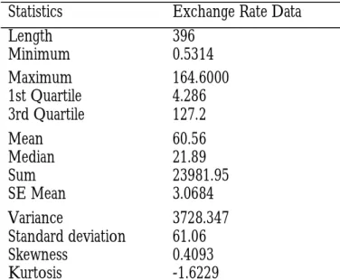
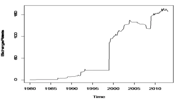
The data were explored with the use of some descriptive statistics (Table 1), station-arity or unit root tests (Table 2) and graphs (Fig. 1, 2 and 3). Table 1 gives the descrip-tive statistics values. Fig. 1 shows that there are no outliers in the data set and Fig. 2 in-dicates that there is a dramatic jump in the
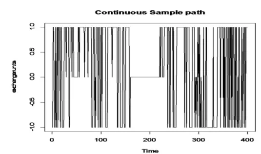
system. The realisation plot (Fig. 3) shows an indication that the variable is non-stationary hence a realization from a nonlinear dynam-ical system. It revealed a dramatic jump in 1999 and that the monthly exchange rate of Nigerian Naira to United States Dollar was highly volatile. Tables 2 which consist of the Augmented Dickey-Fuller and the Phillips-Perron Tests for Stationarity also confirmed that the series is non-stationary. The dra-matic jump in 1999 can be attributed to the political transition from military to demo-cratic government which brought about some changes in policies. Fig. 4 indicates continuous sample paths of the state spaces. It shows that the Nigerian monetary ex-change rate follows a random walk model.
Table 1: Descriptive Statistics of the Exchange Rate Data
Statistics Exchange Rate Data
Length 396
Minimum 0.5314
Maximum 164.6000
1st Quartile 4.286 3rd Quartile 127.2
Mean 60.56
Median 21.89
Sum 23981.95
SE Mean 3.0684
Variance 3728.347
Standard deviation 61.06
Skewness 0.4093
Kurtosis -1.6229
Table 2: Augmented Dickey-Fuller and Phillips-Perron Tests for Stationarity of the data
Unit Root Test Hypothesis Test Statistics p-value Decision Augmented
Dickey-Fuller
H0: The Series is Non Stationary
H1: The Series is Stationary -2.1434 0.5167 Accept Ho Phillips-Perron H0: The Series is Non Stationary
H1: The Series is Stationary -13.8437 0.3357 Accept Ho
Figure 2: Histogram of the Exchange Rate Data
Stationary Analysis
The generating function can therefore be given as trinomial distribution from the
Random Walks. This gives the initial proba-bility of the state of the process as
Figure 4: Continuous Sample path of Nigerian Exchange rate to US Dollar
and the transition probability matrix given as
With the Chapman-Kolmogrov equation, the stationary probability distribution of the sys-tem can be obtained. Using the Chapman – Kolmogorov relation
The absolute Probabilities are given as
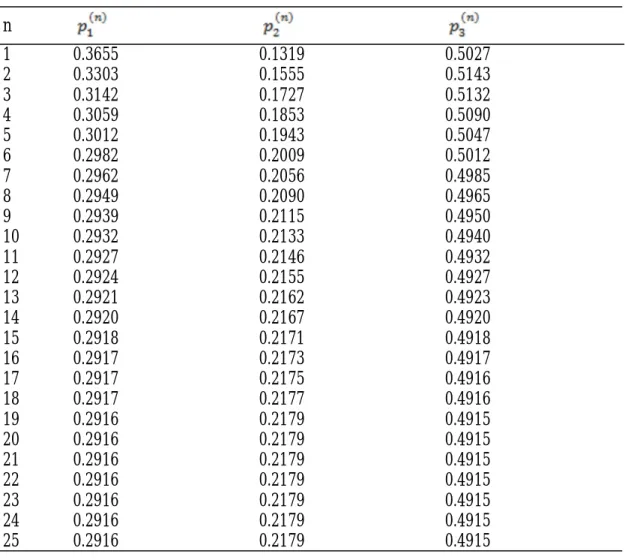
Using the Chapman-Kolmogorov equation recursively, the distribution converges to the fixed probability vector which equals the absolute or stationary probability distri-bution of the system at time, . This is as
shown in Table 3. Therefore the steady state probability distribution of the system which does not depend on the initial probability distribution is
and is the initial probability distribution.
Table 3: Absolute Probabilities of the State of the Systems at time,
n
1 0.3655 0.1319 0.5027
2 0.3303 0.1555 0.5143
3 0.3142 0.1727 0.5132
4 0.3059 0.1853 0.5090
5 0.3012 0.1943 0.5047
6 0.2982 0.2009 0.5012
7 0.2962 0.2056 0.4985
8 0.2949 0.2090 0.4965
9 0.2939 0.2115 0.4950
10 0.2932 0.2133 0.4940
11 0.2927 0.2146 0.4932
12 0.2924 0.2155 0.4927
13 0.2921 0.2162 0.4923
14 0.2920 0.2167 0.4920
15 0.2918 0.2171 0.4918
16 0.2917 0.2173 0.4917
17 0.2917 0.2175 0.4916
18 0.2917 0.2177 0.4916
19 0.2916 0.2179 0.4915
20 0.2916 0.2179 0.4915
21 0.2916 0.2179 0.4915
22 0.2916 0.2179 0.4915
23 0.2916 0.2179 0.4915
24 0.2916 0.2179 0.4915
This implies that the value of Nigerian Nai-ra will at the long run reduce as compared to the US Dollar with a probability of 49%. This dynamics can be better viewed with the use of high frequency data such as weekly, daily or even hourly data of the ex-change rate.
CONCLUSION
Dynamical systems are very common and are considered to be stochastic processes by virtue of their own mechanism. The study considered dynamical system as a random process with independent increments and as a result can be modelled with Markov chains models. The system was therefore viewed as a Random Walk from the state spaces of the Markov process. The Chap-man-Kolmogorov equation gave a straight forward iteration which converges to the stationary distribution of the process. The study shows that the Nigerian exchange rate to US Dollar is ergodic.
REFERENCES
Agwuegbo, S.O.N., Adewole, A.P., Olayiwola, O.M., Apantaku, F.S. 2014.
Signal Model for the Prediction of Wind Speed in Nigeria. Journal of Energy Technologies and Policy 46: 38-44
Akintunde, A.A., Asiribo, O.E.,
Adebanji, A.O., Adelakun, A.A., Ag-wuegbo, S.O.N. 2008. Stochastic
Model-ing of Daily Precipitation of Daily Precipita-tion in Abeokuta Proceedings of Interna-tional Conference on Science and NaInterna-tional Development. 108-118. College of natural Sciences COLNAS., UNAAB, Abeokuta
Aoki, M. 1994. New macroeconomic
mod-eling approach, Hierarchical Dynamics and mean field approximation, Journal of Econom-ic DynamEconom-ics and Control, 18: 865-877
Aoki, M. 1996. New approaches to
macroe-conomic modeling, Evolution Stochastic Dy-namics, Multiple Equilibria and Externalities as field effects, Cambridge University Press, Cambridge
Bailey, N. 1984. The elements of stochastic
processes with applications to Natural Sci-ences, John Wiley and sons, Inc. New York
Davies, M.H.A. 1993. Markov models and
optimizations, Chapman and Hall, London
Devaney, R. 1989. An Introduction to
Cha-otic Dynamical Systems, Addison Wesley
Durrett, R. 1991. Probability: Theory and
Examples, Wadsworth and Brooks, Cole ad-vanced books and software, Pacific Grove
Dynkin, E.B. 2006. Theory of Markov
Pro-cesses, Dover Publications Inc. Mineola, New York
Eckstein, Z., Wolpin, K.I. 1989. The
speci-fication and estimation of dynamic stochastic discrete choice models, Journal of Human Re-sources, 24: 562-598
Feller, W. 1971. An introduction to
proba-bility theory and its applications, Vol. 2, Wiley and Sons, New York
Franke, J., Hardle, W., Hafner, C. 2004.:
Statistics of Financial Markets: An introduc-tion, Springer-Verlag, New York.
Hall, J., Rasmussen, C., Maciejowski, J.
2012. Modelling and Control of Nonlinear Systems using Gaussian Processes with Par tial Model Information; 51st Institute of Electrical and Electronics Engineers (IEEE) Conference on Decision and Control, De-cember 10-13, 2012. Maui, Hawaii, USA
Kalman, R.E. 1960. A New Approach to
Linear Filtering and Prediction Problems. Journal of Basic Engineering, Transactions ASME, Series D 82: 35-45
Lainiotis, D.G. 1971. Optimal nonlinear
estimation, in: Proceedings of Institute of Electrical and Electronics Engineers (IEEE) Conference on Decision and Con-trol, December 1971, Vol. 10, Part 1: 417– 423
Meiss, J. 2007. Dynamical systems.
Scholar-pedia, 22.:1629.
Mowery, O.V. 1965. Least squares
recur-sive differential-correction estimation in nonlinear problems, Institute of Electrical and Electronics Engineers (IEEE) Transactions on Automatic Control 10: 399–407
Neal, S.R. 1968. Nonlinear estimation
techniques, Institute of Electrical and Electronics Engineers (IEEE) Transactions on Automatic Control 136.: 705–708,
Shali, J.A., Akbarfam, J., Bevrani, H.
2012. Approximate solution of the nonlinear stochastic differential equations; International Journal of Mathematical Engineering and Science 14: 53-71
Stark H., Woods, J.W. 1986. Probability
Random Processes and Estimation Theory for Engineers, Prentice-Hall, Engle wood cliff, New Jersey
Tomasz, R., Hanspeter, S., Volker, S., Jozef T. 1999. Stochastic Process for
Insur-ance and FinInsur-ance, John Wiley and Sons, Chichester, New York
Whittle P. 1992. Probability via
Expecta-tion, 3rd edition, Springer, New York. (Manuscript received: 10th November, 2015; accepted: 3rd June, 2017).