Thesis

AN ANALYSIS OF SPECIES DIVERSITY, CORRELATION AND AUTOCORRELATION OF MARINE SPONGES IN MYSTERY BASIN, FLORIDA BAY

By:

Rachel Edwards

Honors Thesis

Geography Department

University of North Carolina at Chapel Hill

ABSTRACT

Most research in and around Mystery Basin, located in Florida Bay, has centered on the ecology including what is present in the environment and their potential roles. Sea sponges are vital to the environment in Florida Bay, but little to no research has centered on their spatial structure. This paper investigates the spatial structure of Mystery Basin including species

Table of Contents

ABSTRACT...2

DECLARATION...4

ACKNOWLEDGEMENTS...4

INTRODUCTION...4

LITERATURE REVIEW...7

METHODOLOGY...10

RESULTS & DISCUSSION...19

CONCLUSION & FUTURE STUDY...25

DECLARATION

This work was written independently from any other works written by either this or other authors.

ACKNOWLEDGEMENTS

Thanks to Drs. Aaron Moody, Chris Martens and Meredith Kintzing for their support and guidance as well as Howard Mendlovitz, Amanda Henley, Phil McDaniel, and Brian Evans for meeting with me at various and numerous times to work through issues. They are the source of much knowledge.

INTRODUCTION

their distribution remains largely unknown because of their high growth rates and losses during environmental change.

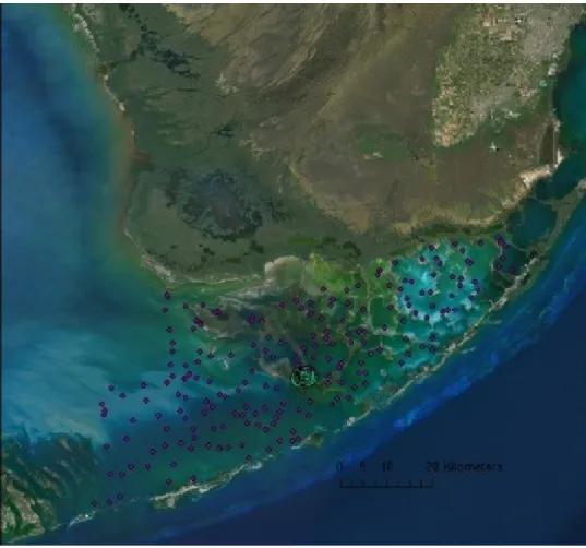
Figure 1: Florida Bay is the body of water located between mainland Florida and the Florida Keys. The purple dots symbolize

Florida's Bay's sampling stations. Mystery Basin, the cluster of green dots, is located inside Florida Bay.

Many roles of sponges in coastal environments have been researched including their biology, habitat for juvenile marine organisms, huge water filtering capabilities, the provision of food for carnivorous animals including hawksbill sea turtles and angelfish and protection of the reef through structural support (Wulff 2001). However, additional research is needed to

can then be compared to chemical and physical data, thereby increasing the knowledge of how sponges may interact with their environment.

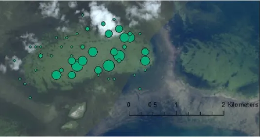
Figure 2: Geodia gibberos in Mystery Basin. The size of the green dots corresponds with the abundance that is found at that sampling station; larger dots mean more abundance was present at the time of sampling.

Three diversity indices will be used to describe species evenness and species richness of the sponge community in Mystery Basin. The indices can then be scaled up to the entire Florida Bay region as first steps to understanding how sponges impact the ecology of the system. Answering these questions will begin to address the wider issue of how sponges affect the biology of Mystery Basin at which point the data can be integrated with chemical and physical data, thereby increasing our knowledge of how the system works. This research may be further scaled up in the future to address similar questions in other water bodies, including tropical oceans where sponges are abundant.

species affect the environment, biology and the ecology at large. It also explores two areas of uncertainty regarding the ecology of sponge communities in Mystery Basin: a) patterns of autocorrelation in the distribution of the four most abundant sponge species, and b) patterns of co-occurrence among these species. Answers to these research questions should fit together to increase the knowledge of Mystery Basin’s ecology. Understanding these patterns and the processes that govern them will lead to better understanding of the biogeochemistry of Mystery Basin and Florida Bay, its consequences of wildlife and human populations, and response to anthropological perturbations. First understanding these processes in Mystery Basin will allow future research to tackle the larger, complex Florida Bay system in a more complete way.

LITERATURE REVIEW

potential to tremendously alter the water column nitrogen biochemistry in Mystery Basin and other ecosystems.

Sponge communities are essential members of the marine ecosystem habitats in which they reside. For example, sponges are essential to mangrove and coral reef systems due to the fact that they filter the water, provide food for carnivorous animals including hawksbill sea turtles and angelfish and protect the reef from falling apart through cementing loose

coral-derived material (Wulff 2001). They are also an important habitat for juvenile lobsters which are able to hide from predators in the massive sponges (Lynch 2000). Human inputs to the

environment can trigger algal blooms, leading to massive sponge die-offs for reasons that are not fully understood (Lapointe 2004). Such die-offs can have widespread effects on many species due to the wide range of roles that sponges play in their environment. However, it is not just the biodiversity of the Florida Keys that are harmed by anthropogenic nutrient enrichment.

Plants including phytoplankton need nutrients, water and sunlight to grow. Of these main factors, the limiting factor is usually phosphorous or nitrogen. Anthropogenic inputs of nutrients into the environment are very harmful as they can raise the amount of that limiting growth factor, thus allowing photosynthetic phytoplankton growth beyond what would naturally occur. This is an algal bloom. Phosphorous has been banned in many forms such as in laundry detergent in recent decades which has significantly decreased the amount of phytoplankton blooms. However, nitrogen is still an issue.

increase light attenuation in the water column, and harm almost every sponge species by removing dissolved oxygen that they need to breathe and clogging their tissues thus preventing normal filtration of smaller food particles. There is evidence of periodic bloom damage at over ninety percent of the sponges in the shallow eastern half of Florida Bay (Peterson 2006). As discussed in Lynch and Philips’ paper, the “susceptibility of Florida Bay to these recurring phytoplankton blooms is due to the large scale loss of filter feeding sponges” (Lynch 2000). Additionally, algal blooms are very harmful to the Florida Bay system’s regional economy. Interestingly, the area surrounding Florida Bay benefits economically from restricting nutrient runoff. The Florida Keys’ tourist industry is dependent upon clear, blue water (Lapointe 2004). An increase in algal growth hurts the tourist industry and thus the area economically because people are less willing to visit areas with murkier water.

Nutrient enrichment and consequent algal blooms can often lead to oxygen depletion or eutrophication. Excessive nutrient inputs cause phytoplankton and other plants to grow quickly and abundantly. As these organisms die, oxygen in the water column is used up in the decay process. This leaves too little oxygen for respiring organisms to breathe, and the sponges suffocate to death. As organisms die, they decay and thereby continue the process of oxygen depletion. This also increases the turbidity of the water column thereby limiting the amount of sunlight that can reach normally healthy photosynthetic organisms.

filtering the water column of the extra phytoplankton. If a sponge survives an algal bloom, it filters phytoplankton out of the water column thereby decreasing the amount of phytoplankton in the water column and lessening the intensity of the algal bloom. Since sponge presence reduces phytoplankton abundance, sponges improve the light penetration of the water column thereby possibly allowing other photosynthetic organisms to live in areas that would otherwise be too turbid.

In general the research on sponges presents data on local community composition and the role of sponges in the ecology of the system. However, little research addresses species diversity of sponges within a given habitat, patterns of co-occurrence between sponge species, and the autocorrelation of individual species. This research intends to fill this gap through the use of methods detailed below.

METHODOLOGY

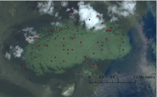
Figure 3: Mystery Basin's sampling sites are symbolized by the red dots where one dot is one sampling station.

At each sampling location, a sponge survey was conducted by three researchers who dove out from a single point using SCUBA; two divers swam directly away from each other while a third diver swam at a ninety degree angle to the first two. Each diver placed a 1x1 meter PVC sampling quadrat at 0, 8, 16 and 24 meters from the common point. The number of sponges, sponge species present, and sponge volumetric measurements were all recorded at each quadrat placement. Other chemical and physical data such as water depth, seafloor bottom type,

conductivity of the water and percent dissolved oxygen were also obtained at each sample site.

The dataset was pre-processed to ensure that it could be used in ArcGIS. The number of individual sponges was added up per species per site to create a single value of sponge

ArcGIS would accept. The locations of each sample site were mapped in ArcGIS as well as what species were located there and in what abundance. Dots were normalized so that the legend of each species was equal; in other words, the sizes of the dots for a given range of abundances are equal for all species to ease visual interpretation. This allows for relative ease in eyeballing abundance and diversity of each classification based on the size dots and how many colored dots are present. The data was further classified into high microbial abundance (HMA), low microbial abundance (LMA) or unknown sponge species (UNK) based on its classification to allow the easy visualization of location, abundance and species richness of each classification.

To visualize what other areas of Mystery Basin and Florida Bay have been surveyed in previous or concurrent studies, the locations of other relevant surveys and sites of data

collections are included in the ArcGIS document. These include the locations of a Florida Bay sponge survey at nearly two hundred points and covering fifteen sponge species; chemical data of twenty-one sites in Mystery Basin; chemical and physical data from 153 sites in Mystery Basin; dissolved oxygen time series data at four sites in Mystery Basin; a survey of sea grass and algae conducted over forty-nine sites; and twelve HOBO pressure sensor measurement locations in and surrounding Mystery Basin. It is useful to have all the available datasets in one location to allow scientists the ability to look in the area of interest to readily see what data has already been collected there.

count of the number of species present in a given area; it does not matter if there is one individual or one hundred present. Thus, it is useful for projects such as conservation efforts when the only knowledge necessary is the overall count of species present. It obviously gives no indication as to the species evenness in that environment. For example, say that two areas each have a species richness of two. The frequency of species 1 and 2 in one area, however, could be 90%-10% while the other area is 50%-50%. This is not indicated by the sites’ shared species richness of two. Therefore, species richness favors uncommon species.

Simpson Diversity Index (D) calculates species diversity in a community in a different way (Fig. 4). D considers both species richness and species evenness although it tends to favor species evenness. It “quantifies the probability that two individuals picked at random from the dataset do not represent the same species” (Tuomisto 2010). For a given richness, D will increase as evenness increases and likewise, for a given evenness, D will increase as richness increases. It is always a value between 0 and 1 where 1 indicates a perfect evenness between species.

Additionally, Simpson is not linear. In fact, a drop from .99 to .97 represents a drop in diversity of 66% (Jost n.d.). Species with a low occurrence do not affect the Simpson value much; thus, it favors dominant species.

D=

_∑

i=1

S

[

]

Figure 4: Simpson Diversity Index equation

on a linear scale, a single Shannon value is quite meaningless unless compared to something else. Shannon’s diversity index considers each species according to its frequency within the community. Because Shannon’s index does not favor either common or uncommon species, it is the fairest of the three diversity measures (Jost n.d.).

H '=−

∑

i=1

S

[

]

Figure 5: Shannon Diversity Index equation

Because Shannon and Simpson are neither on a linear nor the same scale, it is necessary to convert them to “effective number of species” when making comparisons between them (Jost n.d.). The effective number of species indicates the number of species, assuming that all have the same number of individuals, which would be necessary to have the given level of diversity. To determine the number of effective species for Shannon’s diversity index, one must take the exponential of the Shannon value. Simpson’s diversity index can be converted into the effective number of species by taking 1/1-Simpson’s value. Species richness is already in the effective number of species form since it is a count. Once in this form, the three indices can be easily compared.

Many statistical tests exist that will test for relationships between two variables, but it was tricky to find the proper test to determine patterns of co-occurrence between sponge species for this dataset. Pearson product-moment and Spearman rank order correlation tests are two such examples that differ in several important ways. Pearson is a stronger test because it is parametric while Spearman is non-parametric, but Pearson also only tests for a linear relationship whereas Spearman’s test tests for monotonic relationships. The Pearson test can only be used on normally distributed datasets while Spearman’s can be used on any distribution. Although Spearman is a weaker test because it has fewer assumptions than Pearson, it is more suitable for this data because the four sponge species are not normally distributed (Figs. 6-11).

r

=

1

−

6

∑

D

2

^

÷

[

n

(

n

₂

^

₋

₁₎

_]

Figure 6: Spearman's rank order correlation coefficient equation

0 20 40 60 80 100 120 140 160 180

0.000 0.010 0.020 0.030 0.040 0.050 0.060 0.070

Geodia Poisson Regression

Number of Sponges

P

ro

b

ab

ili

ty

0 20 40 60 80 100 120 140 160 0.000 0.010 0.020 0.030 0.040 0.050 0.060 0.070 0.080

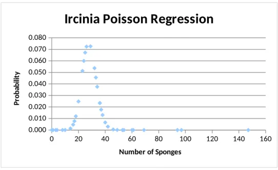
Ircinia Poisson Regression

Number of Sponges

P ro b ab ili ty

Figure 8: Poisson regression curve for Ircinia variabilis

0 5 10 15 20 25 30 35 40

0.000 0.020 0.040 0.060 0.080 0.100 0.120 0.140

Spheciospongia Poisson Regression

Number of Sponges

P ro b ab ili ty

0 50 100 150 200 250 300 0.000

0.020 0.040 0.060 0.080 0.100 0.120

Halichondria Poisson Regression

Number of Sponges

P

ro

b

ab

ili

ty

Figure 10: Poisson regression curve for Halichondria melandocia

Figure 11: Spearman's correlation coefficient significance lookup table

Spearman’s correlation varies from R=-1 to R=1 with -1 representing a perfectly negative relationship, 0 representing no relationship, and +1 representing a perfectly positive relationship. The R value and the number of ordered pairs used to calculate that R value must then be looked up on a table (Fig. 11) to determine its statistical significance; the statistical significance value offers the probability of that correlation for that number of ordered pairs occurring due to chance alone; any significance levels greater than 5% are not statistically significant while those less than 5% are. Spearman’s rank order correlation tests were run on the four most abundant sponge species in Mystery Basin: Geodia gibberos, Ircinia variabilis, Spheciospongia vesparium and

Halichondria melandocia. If a particular site had no individuals of both sponge species, that site was not included in the calculation of the Spearman’s correlation.

The null hypotheses of the Spearman correlations are that no relationships exist between the four most abundant sponge species while the alternative hypotheses are that such

relationships do exist. This is expected because objects in space often either cluster or disperse; objects nearer to each other interact somehow according to the First Law of Geography which states that “everything is related to everything else, but near things are more related than distant things” (Westlund 2013). Thus, as individual species abundance increases, one would expect to see increasing overlap between the species. If this is not found, they can be considered to be either competitors or to prefer different niches in the environment.

displayed by a quantitative variable, in this case sponge distribution (Fortin 1989). It “compares the value of the variable at any one location with the value at all other locations” to determine if the variable is clustered, dispersed or randomly distributed (da Silva 2008). Moran’s I values range between -1 and 1 where -1 indicates a perfect dispersion, 0 indicates a random

arrangement, and 1 indicates clustering. It was run on the four most abundant sponge species:

Geodia gibberos, Ircinia variabilis, Spheciospongia vesparium and Halichondria melandocia. The null hypothesis that Moran’s I tests is that the four sponge species are randomly distributed in Mystery Basin, and the statistical significance of the p-value was designated at 0.05.

RESULTS & DISCUSSION

The Shannon and Simpson diversity indices were run on the Mystery Basin dataset, and species richness was counted. The Simpson’s value for Mystery Basin is 0.98 and Shannon’s value is 3.7. This equals an effective number of species of 40.7 for Shannon and an effective number of species of 50 for Simpson. The species richness- already in the effective number of species form- is 32. The difference between the three measures indicates that sponge species are not evenly distributed spatially in Mystery Basin.

dominant in this dataset over sponges that reproduce more slowly because abundance and not biomass is being measured.

The species diversity measures could be confounded by several factors. One of the thirty-two sponge species that the NSF dataset contains is “unknown.” This could throw off the species diversity measures, particularly species richness since it favors uncommon species. Due to the intrinsic nature of the indices, it is difficult to tell more from these measures without having another habitat to compare it to. Another confounding factor is that the data used in this study dealt with abundance and not biomass. It is possible that there are a high abundance of small sponges while larger sponges such as Spheciospongia vesparium are less abundant. The high abundance of small sponges would indicate dominance in the Mystery Basin ecosystem when calculated this way even though the biomass of larger, less abundant sponges could be greater. Further study of biomass and not abundance would be necessary to look into this further.

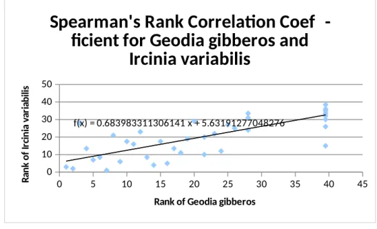
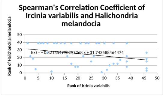
Spearman’s correlation coefficient measures the relationship between two variables. It was run between each of the four most abundant sponge species in Mystery Basin (Figs. 12-17). The significant P-value was set at 0.05; because the P-value for Spheciospongia vesparium and

Geodia gibberos and Spheciospongia vesparium and Halichondria melanodocia were above this threshold, the findings were considered insignificant and no conclusions could be drawn

regarding any spatial structure to their distribution (Fig. 13). Significant negative spatial structure, which indicates that the two species occur in separate sites, was found between

Geodia Ircinia Spheciospongia Halicondria

Geodia

1

0.73

0.33

-0.75

Ircinia

--

1

0.8

-0.4

Spheciospongia --

--

1

-0.38

Halicondria

--

--

--

1

Figure 12: Spearman's results for the four most abundant Mystery Basin species

Geodia Ircinia Spheciospongia Halicondria

Geodia

--

<1%

>5%

<1%

Ircinia

--

--

<1%

1%<x<5%

Spheciospongia --

--

--

>5%

Halicondria

--

--

--

--Figure 13: P-values for the Spearman's results

0 5 10 15 20 25 30 35 40 45

0 10 20 30 40 50

f(x) = 0.683983311306141 x + 5.63191277048276

Spearman's Rank Correlation Coef

-ficient for Geodia gibberos and

Ircinia variabilis

Rank of Geodia gibberos

R an k o f Ir ci n ia v ar ia b ili s

0 5 10 15 20 25 30 35 40 45 0 10 20 30 40 50

f(x) = − 0.46013114496182 x + 33.0579616903878

Spearman's Correlation Coefficient

for Geodia gibberos and Halichondria

melandocia

Rank of Geodia gibberos

R an k o f H al ic h o n d ri a m e la n d o ci a

Figure 15: Spearman's rank order correlation coefficient graph for Geodia gibberos and Halicondria

0 5 10 15 20 25 30 35 40 45

0 10 20 30 40 50

f(x) = 0.870561713319557 x + 3.10348487694909 R² = 0.668863444560604

Spearman's Correlation Coefficient of

Ircinia variabilis and Spheciospongia

vesparium

Rank of Ircinia variabilis

R an k o f Sp h e ci o sp o n gi a ve sp ar iu m

0 5 10 15 20 25 30 35 40 45 50 0 10 20 30 40 50

f(x) = − 0.321354990297268 x + 31.743588464474

Spearman's Correlation Coefficient of

Ircinia variabilis and Halichondria

melandocia

Rank of Ircinia variabilis

R an k o f H al ic h o n d ri a m e la n d o ci a

Figure 17: Spearman's rank order correlation coefficient graph of Ircinia variabilis and Halichondria melandocia

Different sponge species clearly prefer different environments, otherwise sponges in Mystery Basin would not exhibit this non-random spatial pattern. Knowledge of what species prefer what environments will therefore indicate what mini-ecosystems are present in Mystery Basin. For instance, if one knew that a sponge species preferred to live in an area with a very high concentration of a given substance, one would automatically know that that substance was present wherever that species was found.

is also possible that the species simply prefer the same environmental niche, thereby increasing the likelihood that both species would occur in the areas where that niche is present.

The degrees of cohabitation relationships between species in Mystery Basin have ecological significance for the system. It is possible that those species that exhibit positive relationships have symbiotic relationships that allow greater growth or reproduction rates, or that settling in an area where both are present somehow increases the chance of survival for both species. Those species that exhibit negative relationships may be competitors and exist in separate areas so as to make the best use of available resources. This may allow for the most efficient use of resources such as nutrients so that the sponges can maximize growth and

reproduction. As discussed in the results and conclusion section, these ideas require further study to have a better understanding of the reasons for the exhibited relationships between sponges.

The exhibited clustering pattern of Geodia gibberos, Ircinia variabilis and

Spheciospongia vesparium indicates that either something is occurring in Mystery Basin to cause clustering of the three species or that it is advantageous to the species for individuals to be clustered. Perhaps a cluster of individual sponges allows for increased sexual reproduction success; sperm released into the water is more likely to find its way to eggs located closer than those located farther away. Thus, clustered sponges would have a reproductive advantage over those who are not located as closely to individuals of the same species. Lastly, it is possible that clustering occurs from migration outside of Mystery Basin; if, say, a tidal flux brings in a group of sponge larvae, they are all likely to settle in the first habitable area they come to. Further study is required to determine whether the clustering is due to a physical or chemical parameter, migration from outside of Mystery Basin as a result of tidal fluxes or for some other reason.

G eo di a gi bb er os Ir ci ni a va ri ab ili s H al ic ho nd ri a m el an od oc ia Sp he ci os po ng ia ve sp ar iu m

Moran's I 0.162 0.285 -0.014 0.143

z score 2.31 3.885 0.092 1.988

p value 0.0212 0.0001 0.926 0.047

Figure 18: Moran's I results

CONCLUSION & FUTURE STUDY

support highly productive sea grass communities, provide food sources for vast numbers of filter feeding organisms and are the habitat for important commercial species. The region is extremely biologically diverse yet vulnerable to anthropogenic processes associated with the highly

developed tourist industry in south Florida. However, humans do not fully understand this important natural system. If the relationship between the existing species and the ecology is not even known, how can the effects of humans possibly be well understood? They cannot, and that is why the research is necessary.

This paper just scratches the surface of what is possible with this dataset and leaves many questions unanswered. The spatial distribution of sponges in Mystery Basin needs to be further investigated; are sites that are closer together more likely to have similar abundances and species diversity in accordance with the First Law of Geography? Is there evidence of spatial structure with space as a predictor? If so, an inverse relationship between abundances and species diversity as a function of Euclidian distance would be expected. With space as a predictor, the spatial structure of sponges in Mystery Basin could be evidenced with a dissimilarity distance matrix. Mantel tests and permutations could be run on the matrices that have been tested to further evidence spatial structure and indicate whether or not it was due to chance. It would also be interesting to apply co-locational analyses to HMA and LMA sponges and to see if their spatial distribution was due to chance.

similar environmental questions in other water bodies possibly even including larger scale areas in the world’s oceans. In conclusion, sponge distribution and the effects of these actively

REFERENCES

Beals, M., Gross, L., & Harrell, S. (1999). Diversity Indices: Simpson’s D and E. Retrieved from http://www.tiem.utk.edu/~gross/bioed/bealsmodules/simpsonDI.html.

Stevely, J. M., Sweat, D. E., Bert, T. M., Sim-Smith, C., & Kelly, M. (2010). Commercial Bath Sponge (Spongia and Hippospongia) and Total Sponge Community Abundance and Biomass Estimates in the Florida Middle and Upper Keys, USA. Proceedings of the Gulf and Caribbean Fisheries Institute, 62, 394 – 403.

Da Silva, E. C., Silva, A. C., de Paiva, A. C., & Nunes, R. A. (2008). Diagnosis of lung nodule using Moran’s index and Geary’s coefficient in computerized tomography images. Pattern Analysis and Applications, 11(1), 89–99.

Guisan, A., & Zimmermann, N. E. (2008). Predictive habitat distribution models in ecology. Ecological Modelling, 135(2-3), 147–186.

Jost, L. (n.d.). The new synthesis of diversity indices and similarity measures: Effective number of species. Retrieved from

http://www.loujost.com/Statistics%20and%20Physics/Diversity%20and%20Similarity/ EffectiveNumberOfSpecies.htm.

Lapointe, B. E., Barile, P. J., & Matzie, W. R. (2004). Anthropogenic nutrient enrichment of seagrass and coral reef communities in the Lower Florida Keys: discrimination of local versus regional nitrogen sources. Journal of Experimental Marine Biology and Ecology, 308(1), 23–58.

Synechoccus by Three Sponge Species from Florida Bay, U.S.A. (2000). Bulletin of Marine Science, 67(3), 923–936.

Peterson, B. J., Chester, C. M., Jochem, F. J., & Fourqurean, J. W. (2006). Potential role of sponge communities in controlling phytoplankton blooms in Florida Bay. Marine Ecology Progress Series, 328, 93–103.

Drapeau, P., Fortin, M.-J., & Legendre, P. (1989). Spatial Autocorrelation and Sampling Design in Plant Ecology. Vegetatio, 83(1/2), 209–222.

Stevely, J., & Sweat, D. (2008). Florida’s Marine Sponges: Exploring the Potential and Protecting the Resource. Retrieved from http://edis.ifas.ufl.edu/sg095

Thomas, L., Buckland, S. T., Rexstad, E. A., Laake, J. L., Strindberg, S., Hedley, S. L., Bishop, J., et al. (2010). Distance software: design and analysis of distance sampling surveys for estimating population size. Journal of Applied Ecology, 47, 5–14.

Tuomisto. (2010). A consistent terminology for quantifying species diversity? Yes, it does exist. Oecologia, 164(4), 853–860.

Westlund, H. (2013). A brief history of time, space, and growth: Waldo Tobler’s first law of geography revisited. The Annals of Regional Science,51, 917–924. Whittaker, R. H. (1960). Vegetation of the Siskiyou Mountains Oregon and

California. Ecological Monographs, 30(3), 279–338.