1154.pdf

m

ABSTRACT

Many contaminants of concern in the subsurface are volatile. This fact has

been exploited of late in the application of vapor-phase extraction methods for

aquifer rehabilitation. The design of vapor-phase extraction systems may be aided

by use of mathematical models to simulate the restoration process. Because many

common contamination problems are multiphase problems, these simulations often

require the use of compositional multiphase models. A common assumption made in

compositional multiphase models is that individual solute species are in equilibritmi

for all phases present in a system: sohd, aqueous, inamiscible fluid, and vapor. This

work reports on an investigation to characterize the rate of mass transfer between

the aqueous and vapor phases.

A rectangular cross-section experimental apparatus was designed and built to

investigate the rate of mass transfer at the interface between the unsaturated and

saturated zone. Aqueous solutions with the solute toluene were circulated through

a porous media, while depth-averaged aqueous- and vapor-phase concentrations

were measm-ed at the inlet and outlet. Experimental control variables included

the aqueous-phase velocity, vapor-phase velocity, influent solute concentration, and

media size. Data reduction required determination of longitudinal and transverse

dispersivity, which was accomplished using a fluoride tracer method along with a

two-dimensional finite element model.

In addition, a numerical code was developed to model the transport of VOC's in

#

ACKNOWLEDGMENTS

I would like to thank my advisor, Dr C. T. Miller, for his positive outlook

throughout this project. By providing a rare combination of advice and latitude, he

helped make this project a challenging and rewarding experience. I would also like

to thank Randy Goodman for his valuable assistance in developing the apparatus

and in designing the endcaps for the square column. Finally, thanks to Kris for

enduring the crazy schedule that kept me in the lab and at the computer for too

many nights and weekends. This project was ftmded solely by a grant from the U.S.

ͣ

m

TABLE OF CONTENTS

1 INTRODUCTION...l-l

1.1 MOTIVATION... 1-1

1.2 OBJECTIVES...1-3

2 THEORY... 2-1

2.1 INTRODUCTION...2-1

2.2 GROUNDWATER FLOW EQUATION...2-2

2.3 CONTAMINANT TRANSPORT: SATURATED MEDIA . 2-7

2.4 CONTAMINANT TRANSPORT: UNSATURATED ME¬

DIA ... ... 2-14 2.5 COUPLING THE SATURATED AND UNSATURATED

ZONES...2-17

2.6 MASS TRANSFER THEORY ...2-19 2.6.1 FILM THEORY... . 2-20 2.6.2 PENETRATION THEORY...2-21

2.6.3 SURFACE RENEWAL THEORY...2-23 2.6.4 BOUNDARY LAYER THEORY... 2-25 2.6.5 COMMENTS ON MASS TRANSFER THEORIES...2-26

2.6.6 ADDITIONAL COEFFICIENT EXPRESSIONS...2-27

2.7 DIMENSIONAL ANALYSIS... ... 2-29

3 PREVIOUS EXPERIMENTAL STUDIES...3-1

3.1 INTRODUCTION...3-1

3.2 INFLUENCE OF DIFFUSIVITY AND HENRY'S CON¬

STANT ...3-2

3.2.2 HENRY'S CONSTANT...3-5

3.3 DATA FOR NATURAL SYSTEMS... .3-12

4 MATERIALS AND METHODS...4-1

4.1 INTRODUCTION... .4-1

4.2 MATERIALS...4-2

4.3 APPARATUS ...4-5

4.4 ANALYTICAL METHODS ... . 4-9

4.4.1 AQUEOUS-PHASE SAMPLING AND ANALYSIS...4-9

4.4.2 VAPOR-PHASE SAMPLING AND ANALYSIS ...4-14

4.4.3 MEASURING DISPERSIVITIES...4-16

4.5 COMPUTATIONAL METHODS...4-20

5 RESULTS AND DISCUSSION...5-1

5.1 RESULTS: CIRCULAR COLUMN...5-1

5.2 RESULTS: SQUARE COLUMN ... 5-2

5.3 DISCUSSION OF LAB RESULTS...5-12

5.3.1 CIRCULAR COLUMN...5-12

5.3.2 SQUARE COLUMN... . . . . 5-17

5.5.2.1 Mass Balances...5-17

5.3.2.2 Concentration Effects...5-18

5.5.2.3 Vapor-Phase Velocity ... 5-20

5.3.2.4 Upper- and Lower-Bound Estimates for ki...5-21

5.4 COMPARISON OF THE COMPUTER CODES...5-28

5.5 Computer Simulation Under Ambient Conditions...5-32

6 CONCLUSIONS AND RECOMMENDATIONS . . 6-1

7 APPENDIX A ... 7-1

7.1 NOTATION... 7-2

7.2 REFERENCES... 7-6

8 APPENDIX B . . . . ... ... 8-1

8.1 ANALYTICAL SOLUTION... 8-2

8.2 NUMERICAL SOLUTION... 8-4

8.2.1 SATURATED DOMAIN... 8-4 8.2.2 UNSATURATED DOMAIN... 8-5

#

LIST OF FIGURES

2—1 Differential Volume of Saturated Porous Media...2-3

2—2 Differential Volume for Contaminant Transport...2-8

3-1 k'l/k^^ vs D: Based on Data From Rathbun and Tai (1988b)...3-8 3-2 ki/k^" vs He: Based on Data From Rathbun and Tai (1988b) .... 3-10

3-3 Estimated A;|/A;,°^ vs Experimental ki/k^''...3-11

4-1 Schematic of Laboratory Apparatus...4-6

4—2 Circular Column...4-8

4—3 Longitudinal Cross-Section of Square Column and an Endcap...4-10

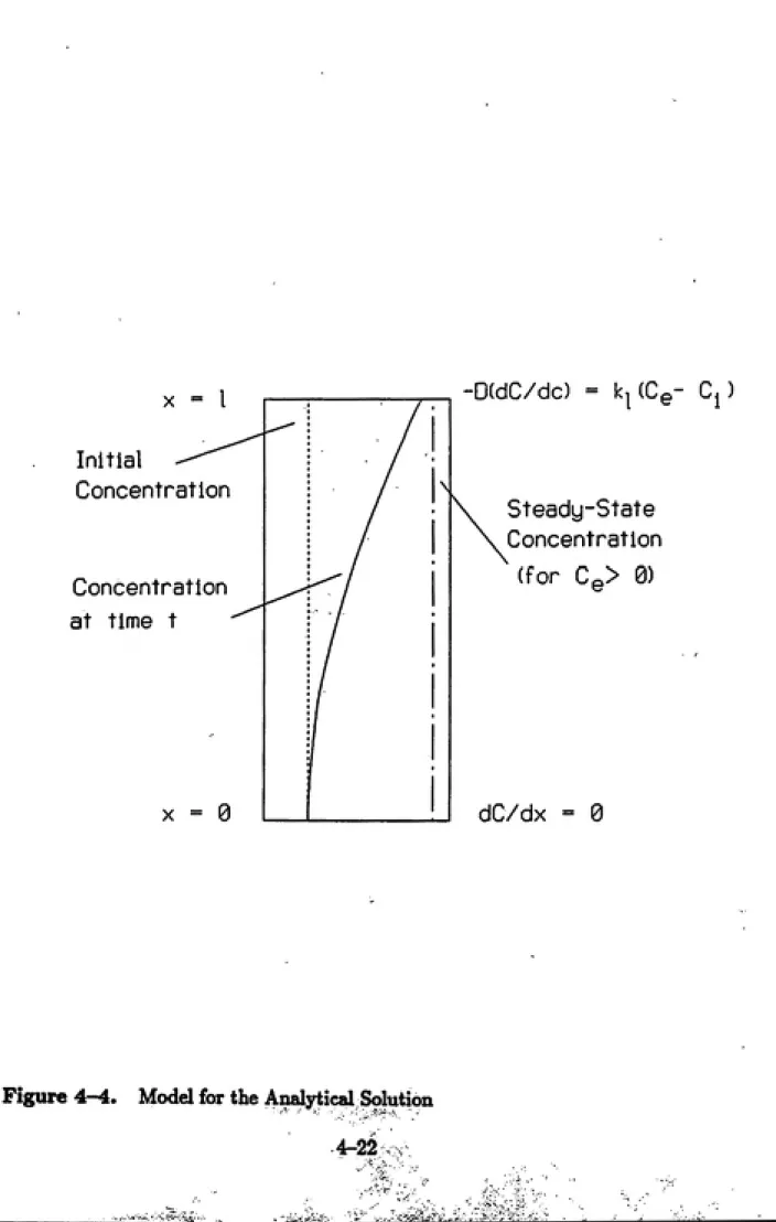
4—4 Model for the Analytical Solution...4-22 5—1 Mass Balance vs Pore Velocity...5-5 5—2 Mass Balance Based on Average Interphase Mass Transfer Rates . . . 5-6

5—3 Normalized Effluent Concentration vs Influent Concentration...5-9

5—4 Optimal Upper- and Lower-Botmd ki with Best-Fit Curves...5-11 5—5 Individual Upper-Bound Values and Confidence Intervals ...5-13

5—6 Determining an Optimal Lower-Bound Value for A:/...5-15

5—7 Individual and Optimal Lower-Bound fc/: Circular Column...5-16 5-8 Normzilized Interphase Mass Flow Rate...5-19

5-9 Lower-Bound Values for Transverse Dispersivity...5-22

5-10 Optimal A;/ as a Function of Pore Velocity and at...5-24 5—11 A Comparison of Results from Both Columns ...5-25

5-12 Sherwood Number vs Reynolds Number for Various dt's...5-27

5-13 ki from the Numerical and Analytical Codes...5-30

5-14 Best-fit Power Functions for A;/...5-31

5-15 Approach to Equihbrium in the Vapor Phase at the Interface . . . . . 5-35

5—17 Approach to Steady-State and to Equilibrium: x = 2.0 days... 5-38 5—18 Approach to Steady-State and to Equilibrium: x = 5.0 days... 5-39 5—19 Approach to Steady-State and to Equilibrium: x — 9-0 days... 5-40

8-1 Validation of the Numerical Code for Mass Transfer... 8-8

LIST OF TABLES

3—1 Parameter Values For Analysis of Data from Rathbun and Tai (1988b) 3-6 3—2 Comparison of Experimental and Estimated Values for k\/ki ^ .... 3-12

4-1 Measured Properties of Glass Beads... 4-4

5-1 Lower-Bound Values for ki: Circular Column... 5-2

5—2 Lower-Bound kf. Circular Column ... 5-3

5—3 Statistics for Linear Regressions of Ce/C, vs C,-... 5-8

5—4 Statistics: Linear Regressions of Ce/C^ vs Vapor Velocity... 5-10

5—5 Upper-Bound and Lower-Bound ki: Square Coliunn... 5-12

5—6 Upper-Bound ki from Both Computer Codes... 5-29

5—7 Conditions and Parameter Values for Simulation... 5-33

1 INTRODUCTION

1.1 MOTIVATION

Groundwater is an essential resovtrce in the United States. It is vital for in¬

dustrial and agricultural purposes, and approximately half of the population uses

groundwater for residential purposes. Rural areas and urban centers in arid regions rely heavily on groundwater. In fact, the allocation of scarce groundwater resources may become one of the most important political issues in the arid regions of the

American Southwest.

However, the industrial nature of America's economy threatens the quality of groundwater throughout the nation. Spills during the production, transporta¬ tion, and storage of hazardous chemicals can poUute the subsurface. Lealcs from

hazardous waste treatment, storage, and disposal facilities can also introduce pollu¬

tants. For these reasons, the quality of groundwater resources in the United States increasingly commands the attention of the pubHc and those who formulate public

policy.

Of the many compounds that pose a threat to groundwater quality, one of the

most significant classes of chemicals is volatile organic compotmds (VOC's). VOC's

are a great concern for a ntimber of reasons. The primary reason is that many

of the most common VOC's are hazardous to himian health. One VOC, benzene,

is a known himian carcinogen (Aksoy, 1988). Several others are known animal

carcinogens and are suspected human carcinogens. Virtually all VOC's exhibit

some toxic characteristics.

From the perspective of groundwater quality, an equally disturbing fact is that

persistent in the environment. In this respect, chlorinated VOC's are particularly

problematic. These compounds have been used widely as industrial solvents and

degreasers, as well as for dry cleaning operations. They have been introduced into the substirface throughout the United States. Unless remedial measures are taken,

they will remain there and spread for a long time.

Finally, VOC's are ubiquitous. The acronym "VOC's"includes chemicals that

are used for dry cleaning, for industrial degreasing, as industrial solvents, and as fuel components for automobiles and airplanes. Undoubtedly, automobile gasoline is the VOC blend that most people in the United States encounter on an almost daily basis. It is illustrative of the omnipresence of VOC's in our society and the threat they pose to groundwater quality. In most urban areas one can find ga^

stations at virtually every major intersection, and it is not imcommon to find more than one per intersection. Furthermore, until very recently, gasoline was stored at

these stations in undergroimd tanks that were designed and operated with minimal

concern for leakage.

Because VOC's are a significant threat to groundwater quality, hydrogeologists and engineers have been working to develop both accurate methods to model the

fate and transport of VOC's and effective designs for removing these compounds

from the subsurface. The purpose of this study was to test a key assumption that is

presently used in models simulating the transport of VOC's. The motivation for this research was to improve the accuracy of these models, to elIIow for better prediction of fate and transport, and to enable more informed decision-malcing when choosing

m

1.2 OBJECTIVES

This study had four objectives. All of the objectives centered on an analysis of the assvmiption that the liquid in the saturated domain and the vapor in the unsaturated domain are at equilibrium at the saturated-unsaturated interface. The

first objective was to develop a methodology for generating laboratory data to quantify the rate of interphase mass transfer imder conditions approximating those in the subsurface. The second objective was to generate such data for a single VOC. The third objective was to use the lab data for the VOC to test the assumption of equilibrium under ambient subsurface conditions. The final objective was to determine conditions under which the equilibrium assumption may not be valid for

2 THEORY

2.1 INTRODUCTION

This chapter presents derivations of the equations that described the physical

system modeled in this study. The equations governed the processes of interest in the subsurface. In simplified form, they modeled the conditions in the lab apparatus. In its most general form, the model had two dependent variables in the saturated

zone and three dependent variables in the unsaturated zone.

The physical processes governing the transport of a contaminant in the sub-svirface for this study were: bulk transport, diffusion and dispersion, degradation

reactions, zind interphase mass transfer. In the saturated zone, the transport of wa¬ ter was assumed to be unaffected by the aqueous phase contaminant concentration. In the unsaturated zone at ambient conditions, density driven natural advection of the vapor phase was not considered significant. Finrthermore, for conditions of

forced advection of the unsaturated zone vapor phase, the bulk transport was as¬

sumed to be independent of the vapor phase contaminant concentration. For these reasons, the equations governing bulk transport were decoupled from the contami¬

nant transport equations and are discussed only briefly in section 2.2. The governing

equations for transport in the saturated and unsaturated zones are derived in sec¬

tions 2.3 and 2.4. The equations in these two domains were coupled by equating

the fluxes at the shared interfacial boundary; the mathematics of this coupling are

discussed in section 2.5. General interphase mass transfer theory is presented in sec¬

the method is applied to obtain possible correlations for mass transfer coefficients

in the subsurface.

2.2 GROUNDWATER FLOW EQUATION

The groundwater flow equation can be derived by writing a mass balance on a

differential volume of completely saturated porous media. This follows the method

of Bird et al. (1960) for deriving the equation of continuity. A differential volume is

shown in Figure 2-1. iVj, Ny, and N^ are the mass fluxes in the principal directions

and Ax, Ay, and Az are the incremental lengths. The mass balance on the voltmie

can be written as

[MASS RATE IN] - [MASS RATE OUT]

= [MASS RATE OF ACCUMULATION]

(2-1)

In mathematical terms, this is

{N^\r-N^\x+Ax)AyAz + (Ny\y-Ny\y+^y)AxAz

/XT I »r I w A AxAyAzAinp) (2-2)

+ {N,U-N,U+Az)AxAy=---^^^ ^ ^^

where n is the porosity of the media and p is the fluid density. Dividing equation

(2-2) by the differential volume, AxAyAz, yields

Nr\x-N^\z+Ax , Ny\y-Ny\y+^y , N,\, - N,],+^, _ Ajup)

Ax ^ Ay + A'z -~Ar ^^~^^

From the definition of the differential operator, taking the limit as Ax, Ay, Az,

Ax

'X

N

dN. dNy dN, _ d{np) ^2-4)

dx dy dz dt

Substituting

qiP = Ni (2-5)

into equation (2-4) where qi is the specific discharge (that is, the superficial face

velocity) in the direction i yields

d{qxp) djqyp) d{q,p) ^ d{np)

dx dy dz dt ^ '

Assuming the fluid is incompressible, or assuming the spatial derivatives of p are small compared to the spatial derivatives of the specific discharge, yields

At this point, Darcy's law is introduced. Henry Darcy, a nineteenth-century

French engineer, determined the following empirical relationship for the specific

discharge, g^, the hydratilic conductivity, K, and the spatial derivative of the

piezo-metric head, <p, in one dimension (Bear, 1979)

,. = -irf (2-8)

where i, j, £ind k represent the three principal directions in rectangular coordinates. Equation (2-9) reveals the hydraulic conductivity as a second-rank tensor. It has

been shown that the hydraulic conductivity tensor is symmetrical (Marsily, 1986),

thus

Kij=Kji (2-10)

Dividing equation (2-7) by p and substituting equation (2-9) for the specific

discharge yields

dz \ dx dy dz J p dt

Expressing equation (2-11) more elegantly in vector-tensor notation yields one

form of the groundwater flow equation

V.(KV#)=1^ (2-12)

To write the equation with a single dependent variable, <f>, the right side of equation

(2-12) can be expressed in terms of a specific storage coefficient, 5,. The expression

for Sa is derived by considering the balance of forces that must exist between the soil and the water at some point in an aquifer and the total mass of material above that point in the aquifer (Bear, 1979). The expression is

ld(np)_gdl

Wlth

Sa = gp[{l - n)Km + nK„,] (2-14)

where g is the gravitational constant. Km is the compressibility of the soil matrix,

and Ku, is the compressibility of water. Substituting the right side of equation (2-13)

into equation (2-12) yields

V-(KV(^) = 5,^ (2-15)

which is a common form of the groundwater flow equation. Equation (2-15) relates changes in the piezometric head in an aquifer to the storage capacity of the aquifer. Returning to the general form of Darcy's law, equation (2-9) , and expressing

it in vector-tensor notation gives

{q} = - [K] {V<f>} (2-16)

Since the pore velocity, v,-, is defined in terms of the superficial velocity and the

porosity by (Bear, 1979)

vi = ^ (2-17)

Darcy's law can be expressed in terms of the pore velocity as

{v} = -hK]{V<f>} (2-18)

This final expression relates the spatial derivatives of piezometric head to the pore

2.3 CONTAMINANT TRANSPORT: SATURATED MEDIA

The contaminant transport equations for the saturated domain axe derived in

this section. The introduction to this chapter explains why the groundwater flow equation and the contaminant transport equation were decoupled for the model used in this study. In addition to assuming that the liqmd-phase flow field was

unaffected by changes in the contaminant concentration, the model assumed that the liquid-phase flow field was fully characterized and at steady-state.

As in the previous section, the governing equation is obtained, after Bird et al.

(1960), by performing a mass balance on a differential volume of satvirated porous

media. In this section, however, the mass balance is on a contaminant rather than

on the fluid phase. The contaminant can be in either the liquid phase or the solid phase, thus two mass balances must be written. The liquid-phase mass balance is

developed first.

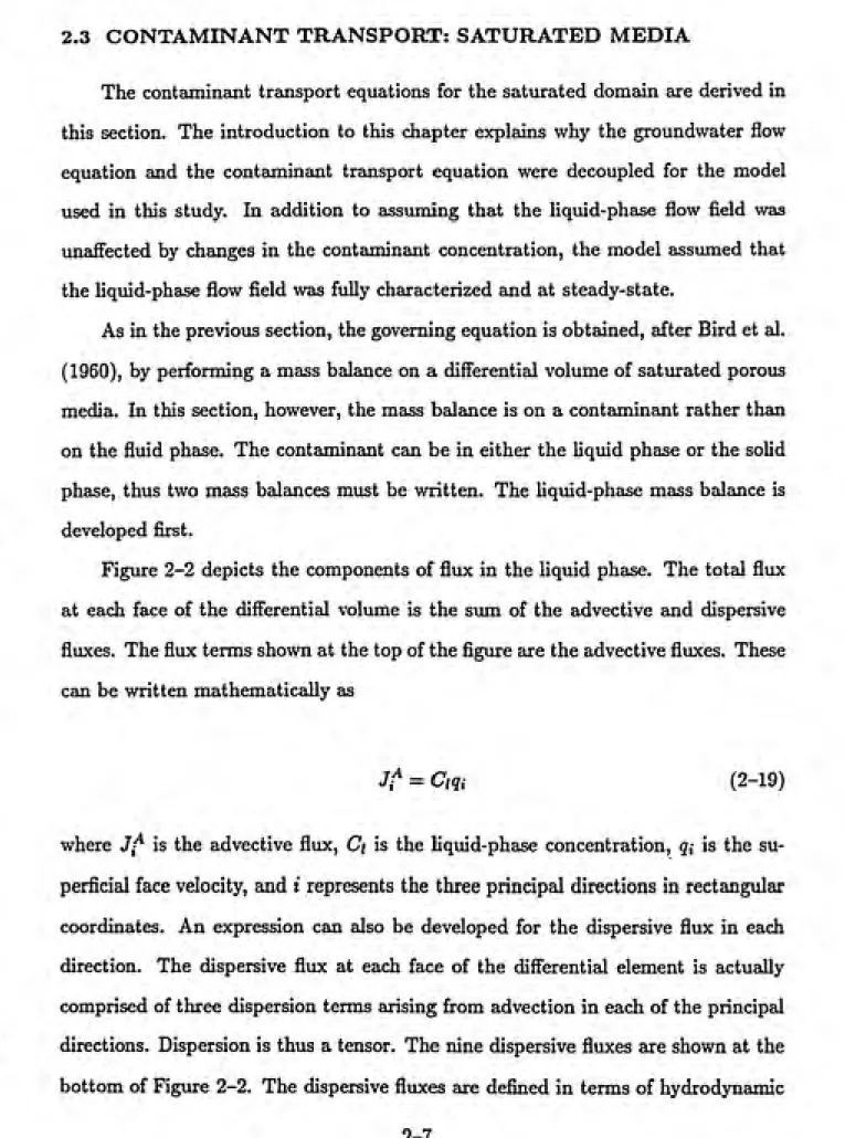
Figure 2-2 depicts the components of flux in the liquid phase. The total flux at each face of the differential volume is the sum of the advective and dispersive fluxes. The flux terms shown at the top of the figure are the advective fluxes. These

can be written mathematically as

J,"" = Ciqi (2-19)

where J,^ is the advective flux, Ci is the liquid-phase concentration, qi is the su¬

perficial face velocity, and i represents the three principal directions in rectangular

coordinates. An expression can also be developed for the dispersive flux in each

direction. The dispersive flux at each face of the differential element is actually

comprised of three dispersion terms arising from advection in each of the principal directions. Dispersion is thus a tensor. The nine dispersive fluxes are shown at the

Ax

Ax

1°

'xx xy

/ / /

yx 1^ yy ^ yz

J° J° J°

^ zx ^ zy ^ zz

Az

Ay

dispersion coefficients, which are comprised of mechanical dispersion and molecular

difFusivity. Bear (1979) defined the hydrodynamic dispersion tensor, D/,, by

Dfc,.-j = atvSij + (ai - «<) ^ + Dinr (2-20)

where 6ij is the Kronecker delta, n is the porosity of the media, r is the tortuousity of the media (0 < r < 1.0), a/ and at are the longitudinal and transverse dispersivities

for the media, and

V = ^vl +vl + vl (2-21)

with Vx, Vy, and Vz being magnitudes of the macroscopic pore velocities in the

principal directions.

The total dispersive mass flux of contaminant in the principal directions is

expressed as

tD_ Jr. dCi dCi dCi\

^° = -"Kf+^.,„f+^M.§) (2-23)

Combining the advective and dispersive fluxes, equation (2-19) and equations

rT \ ^ (r. dCi „ dCi ^ dCi\

Ji =n VyCl - I Dh,yx-^- + Dh,yy-^- + Vh,yz

dec

dx

dCi

dy dz

rT \ ^ fr. dCi ^ dCi „ dCi\

(2-25)

(2-26)

(2-27)

#

Now the liquid phase mass balance can be written in terms of the total mass fitix in the principal directions. The mass balance can be expressed verbally as

[MASS RATE IN] - [MASS RATE OUT]

+ [MASS RATE OF REACTION] (2-28)

= [MASS RATE OF ACCUMULATION]

Note that this mass balance contains one more term than the bulk fluid phase mass balance in the previous section. This reaction term represents sources and sinks

within the domain. For a soiirce (e.g., a solid desorbing contaminant into the liquid

phase) the term is positive. For a sink (e.g., chemical or biological degradation

within the liquid phase) the term is negative. Writing the mass balance mathemat¬ ically, in terms of the total fluxes J?^, yields

(Jllx - JjU+Ax)AyA2r + {Jj\y - J^\y^^y)AxAz + {JJU - JjU+Az)AxAy

nACi\ AxAyAz{nACi)

+

At At

(2-29)

Dividing through by the volume, AxAyA^:, and taking the limit as the A's go to

#

Substituting equations (2-25) to (2-27) into equation (2-30) and writing the result

in vector-tensor notation yields the governing equation for contaminant transport

in the liquid phase

__ = _i;. VC, + V • (DfcVCO + ( ^ ) (2-31)

Equation (2-31) is often referred to as the advective-dispersive-reactive (ADR) equation. The reaction term in equation (2-31) includes interactions between the

soUd and liquid phases as well as homogeneous reactions in the liquid phase

dCi

dt _{en \ ^" / rxn \ / rxn}

= (f)'"'-(f)"

Before the liquid phase governing equation can be completely defined, the solid phase governing equation must be considered. In this study, sorption onto the solid

was modeled as a two-site phenomenon. This model (Cameron and Klute, 1977)

postulates that two types of sorption sites exist on the solid phase: 'fast' sites and 'slow' sites. Sorption at the fast sites is an equilibrium process, while sorption at the slow sites is a mass transfer limited process. The total solid phase concentration,

Qa, is

qs = qss + q/s (2-33)

where 5,, is the solid phase concentration for the slow sites and 5/, is the solid phase

concentration for the fast sites. For both slow and fast sorption, linear equilibrium

qfs = K.fCi (2-34)

where Ke,f is the fast site equilibrium constant. A mass balance on the fast sites

yields

fdqf3\ ^ dqjs _ fdqfA

V^A.p dt V^A.„ (2-35)

= Kef-~- + krfKefC,

where krf is a first-order rate constant for degradation reactions at the fast sites.

The two terms from the mass balance on the fast sites are incorporated into the

liquid phase governing equation. The mass balance for the slow sites on the sohd

phase is

^ = ks {K,sCl - qss) - krsQss (2-36)

where k^ is the mass transfer coefficient for sorption at the slow sites, K^s is the equilibrium constant for sorption at the slow sites, and krs is the first-order degra¬

dation constant at the slow sites (Weber and Miller, 1988). Equation (2-36) is one

of the two governing equations for the saturated zone.

The term in equation (2-32) describing the interactions between the sohd and

liquid phcises can now be expressed as

(f)

= --Kef^ - ^krfK.fCi -kA (K^sC, - 9„) (2-37)

comprised of: equilibrium sorption at the fast sites; first-order degradation on the

solid at the fast sites; and mass transfer limited sorption at the slow sites.

Substituting equation (2-37) into equation (2-32) , then placing the resulting

expression in the ADR equation yields the liquid-phase governing equation with all

of the terms now explicitly defined

- ^KsK.fCi - kAiK^sCi - qss) - -Kef —

dCA'"

dt J/ rxn _(2-38)

The last term on the right hand side of equation (2-38) caji be moved to the left

hand side and the retardation factor, /?/, can be defined by

Rf=(l + ^K\f^ (2-39)

Writing Equation (2-38) in terms of Rf and assuming a first-order reaction for

homogeneous liquid-phase degradation yields the final version of the liquid phase

governing equation

^ (2-40)

-^krsKefC,-kA{KesC,-qss)

where kri is the first-order rate constant for liquid-phase reaction. This expression

constitutes the remaining governing equation for the saturated zone.

The ADR equation and the the solid-phase slow-site equation , equations (2-40)

and (2-36) respectively, axe the two significant equations derived in this section.

Simultaneous solution of the equations, with appropriate boundary and initial con¬

ditions, described the movement of contaminant within the saturated zone. The

2.4 CONTAMINANT TRANSPORT: UNSATURATED MEDIA

Modehng the movement of contaminant in the imsaturated domain requires the

simultaneous solution of three equations. The equations arise from mass balances

on the three phases in the unsaturated zone and axe coupled by interphase mass transfer terms. The assumptions that define the processes included in the model

used for this study and that determine the form of the governing equations are:

• the vapor phase is the only mobile phase in the luisaturated zone;

• the vapor-phase flow field is known and is unaffected by changes in vapor-phase

concentration;

• concentration gradients in the vapor phase do not induce natural advection; • the aqueous phase completely wets the solid phase, thus no vapor-solid inter¬

phase mass transfer occurs;

• vapor-Uquid interphase mass transfer is a nonequilibrium process;

• the equilibrium relationship between the vapor and liquid is defined by Henry's

law;

• liquid-solid interphase mass transfer follows the two-site, linear equilibrivmi

sorption model (Cameron and Klute, 1977); and

• first-order degradation reactions can occur in the liquid phase and at both the

fast and slow sites on the solid phase.

Prom the assumptions above, it is clear that the equations for the solid phase

in the unsaturated zone are the same as the solid phase equations for the satiu-ated

zone. The total solid phase concentration, q^i is the sum of the concentrations at

the fast and slow sites

where the fast site concentration is solely dependent upon the liquid phase concen¬

tration and the fast site equilibrium constant

g/„ = K.fCr (2-42)

the mass balance for the fast sites is

(dqfu\ ^ dqfu _ (dqfu\

V ^ Arp ^ \^ Jrr. (2-43)

where Kef is the fast site equilibriiun constant and krf is a first-order rate constant

for degradation at the fast sites. The mass balance for the slow sites is

^ = k^iKesCj" - qsn) - krsqsu (2-44)

where kg is the slow site mass transfer coefficient, K^g is the slow site equilibrium sorption constant, and krs is a first-order degradation constant for the slow sites. Equation (2-44) is one of the governing equations in the unsaturated zone.

Since the aqueous phase is immobile, the aqueous-phase mass balance in the

unsaturated domain does not contain advection or dispersion. However, it does include all of the reaction terms that appear in the saturated zone aqueous-phase equation plus one additional term. The additional term is for the vapor-liquid interphase mass transfer that occurs within the unsaturated zone. This term is

where Kia is the mass transfer rate constant for vapor-liquid mass transfer within

unsaturated zone, and He is the Henry's constant for the contaminant. Henry's law

is

C: = HcC! (2-46)

where the asterisk superscripts denote equilibrium values.

In summary, the terms that appear in the aqueous phase mass balance in

the unsaturated zone describe: first order homogeneous degradation; liquid-vapor interphase mass transfer; slow sorption; fast sorption; and first order degradation

at the fast sorption sites. The equation is

dt 'ͣ'^' V SI

-te)^'(^"^"--^-^^-(^) ''-"''

^' -KfK^fCr

By moving the fast sorption term to the left side of equation (2-47) , the mass

balance can be expressed in terms of the retardation factor, Rf,

5C" /1 — S"" \

^) k,{KesCr - qsu) - :^KfK.fCr

(2-48)

'u;

where Rf is defined here by

Equation (2-49) is the second of the three governing equations in the unsaturated

m

m

The fined equation to consider is the vapor-phase mass balance. Since the vapor phase is mobile, the governing equation will include the advection and dispersion terms that were defined in the previovis section for the mobile water phase in the

saturated zone. The vapor phase does not include a homogeneous degradation

reaction term, but it does include the expression for vapor-liquid interphase mass

transfer within the tuisaturated domain. The governing equation for the vapor

phsise in vector-tensor notation is

^ = -vt • Va -H V • (D^ VC„) - Kia^iC - HcCf) (2-50)

Equations (2-44) , (2-48) , and (2-50) were the three governing equations for

the unsaturated zone. Simultaneous solution of these equations with appropriate

boundary and initial conditions described the transport of contaminant within the

unsaturated zone.

2.5 COUPLING THE SATURATED AND UNSATURATED ZONES

The equations presented in the two previous sections describe the transport of

a contaminant within each of two domains: the saturated zone and the unsaturated

zone. A contaminant that partitions between the aqueous and vapor phases couples

the two domains, and modeling the transport of such a contaminant requires that

the systems of equations be solved simultaneously. Since the two domains only

interact along a single shared boimdary, the governing equations for the two domains must be coupled by imposing appropriate boundary conditions. Specifically, the flux of contaminant normal to the interface at the boundary must be equal for the liquid in the saturated zone and the vapor in the unsaturated zone. Mathematically,

m

Nonequilibrium interphase mass transfer is typically expressed as a fimction of a driving force and a mass transfer coefficient. Thermodynamics reveals that two phases in contact will approach the same fugacity; stated less esoterically, the two phases will approach equilibrium. For this reason, the driving force used in mass transfer expressions is the deviation from equilibrium. The equilibritun expression

used in this study is Henry's law

C: = H^Cr (2-52)

where He is Henry' constant, the subscripts indicate vapor and liquid phases, and the asterisk superscripts denote equilibrium values. Henry's law is applicable for a

dilute solution in equilibrium with an ideal-gas mixture (McCabe and Smith, 1976).

The flux at the interfacial boundary in the liquid phase of the satiu-ated zone, defined in terms of a mass transfer coefficient, is

where Ki is the overall mass transfer coefficient at the interface, based on the

liquid phase, and Dj/ is the transverse dispersion coefficient governing the flux of

contaminant within the liquid phase normal to the interface. Likewise, the flux at the interfacial boundary in the vapor phase of the unsattirated zone is

where n, is the porosity in the saturated zone, Uu is the porosity in the unsaturated

#

m

the vapor pha^e normal to the interface. Note that the mass transfer coefficient and

the expression for the driving force axe identical in equations (2-53) and (2-54) .

Combining these two terms with the porosity and water saturation terms ensures

mass balance at the interface. The inclusion of two different porosity terms for the

saturated and vmsaturated zones may appear unnecessary since one could assume

that the porosity in the subsurface does not vary greatly over the short distance

represented by the two sides of the interface. This may be a reasonable assumption

in modeling the subsurface. However, the different porosity terms were necessary

for modeling the laboratory apparatus used in this study since the unsatvirated zone

was a continuous vapor phase and, therefore, had a porosity of one.

Specifying the above bovmdary conditions for the liquid-phase governing equa¬ tion in the saturated zone and for the vapor-phase governing equation in the un¬

saturated zone coupled the two domains. Thus, the equations developed in the two previous sections and the boundary conditions presented here constitute a complete

mathematical model for combined saturated-unsaturated transport of a contami¬

nant which partitions between the aqueous and vapor phases.

2.6 MASS TRANSFER THEORY

Throughout this centtiry, engineers have expended much effort generating meth¬ ods for relating mass transfer coefficients to the hydrodynamics of mass transfer

processes. Both empirical and theoretical approaches have been taken. Empirical

methods have generally been used for the design of engineered systems. However,

engineers have formtilated a large number of theoretical models because these mod¬

els are nominally appUcable to a wide range of systems, and they engender the feeling that imderlying mechanisms have been explicated. Of the many theories of

All of the models presented apply only for dilute systems. One empirical approach

to predicting mass transfer coefficients is presented in section 2.7.

2.6.1 FILM THEORY

The simplest theory proposed to explain resistance to interphase mass transfer is film theory, sometimes known as Lewis-Whitman film theory. This theory postu¬

lates that all the resistance to mass transfer restilts from stagnant layers that exist

at interphase boundaries (Lewis aind Whitman, 1924). Mass can only cross the film

by diffusion, thus the mass transfer coefficient is a function of the film thickness

and the difFusivity

ki = -f- (2-55)

where ki is the film mass transfer coefficient for phase i, D^^ is the difFusivity of

component a inside the film in phase i, and li is the thickness of the film in phase i.

At fiuid-fluid interfaces, each phase may have an associated film coefficient, and the

overall resistance to mass transfer across the interface is the sum of the individual

resistances. One problem with the film theory that is immediately evident is the

need for an estimate of the film thickness. Rarely can a rehable estimate of /, be

obtained. Another problem is that the theory compares unfavorably with existing

data. Equation (2-55) predicts that the mass transfer coefficient varies linearly

with difFusivity, while a significant body of experimental data, some of which is

discussed in the following chapter, indicates that the exponent on difFusivity should

2.6.2 PENETRATION THEORY

One theory of interphase mass transfer that eliminates the need for determining the elusive stagnant film thickness was first developed by Higbie (1935). This model is known as penetration theory. The theory can be illustrated by considering a falling liquid film with a wall on one side and a vapor on the other side. The film moves in the x-direction, and interphase mass transfer occurs in the z-direction,

normal to the direction of flow. This model does not postulate a stagnant layer on either side of the interface. However, it does require the following assumptions:

• advection dominates diffusion in the direction of flow, the x-direction; • diffusion dominates advection in the ^-direction;

• the falling film is thick compared to the depth to which mass from the vapor

penetrates;

• the vapor concentration is unchanged along the contact path; and

• the liquid at the interface is in equilibrium with the vapor throughout the

contact length.

The second assumption implies that the liquid is in laminar flow; thus this model has no need to postulate a stagnant film at the interface since the entire film

is essentially stagnant in the 2-direction. The third assumption can be expressed mathematically as a boundary condition at the wall

dCi

-^ = 0 , for 2 = 0, X > 0 (2-56)

which imphes either a thick film or a short contact time. Applying the above

J/Ut = y^(c,,-Cr) (2-57)

where Di is the difFusivity in the hquid, v^ is the liquid velocity at the interface, Cib is the constant bulk liquid concentration some distance from the interface, and C* is the interfacial liquid concentration that is in equilibrium with the vapor phase.

For the parabolic flow field that exists in laminar flow, the term Vm is the maximimi

velocity and is equal to (3/2)i;a, the average liquid velocity. Integrating equation

(2-57) over the entire contact length, L, and dividing by the contact length yields

an expression for the average interfacial mass flux, Ji\int

The liquid-phase mass transfer coefficient, A;/, based on the average flux appears in

the equation

Jilint = kiiCib - CI) (2-59)

Comparing equations (2-59) and (2-58) reveals an expression for the liquid phase

mass transfer coefficient as a function of the hydrodynamics

*,=2y'^ (2-60)

One problem with this model is the need to determine the contact time, Ljvm- In complex systems, this term may be difficult to measure. Note, however, that the

mass transfer coefficient varies as the square root of the difFusivity. This result com¬

in packed columns. This is surprising since the model would seem to be limited by

the assumptions of short contact time, thick liquid film, and Iziminar flow. Higbie,

however, developed this theory for use in modeling packed process vmit operations.

He proposed that the fluid moves in laminar flow across individual packing elements

and mixes at the points where these packing elements meet.

2.6.3 SURFACE RENEWAL THEORY

A niunber of models exist that do not have the assiunptions about flow regime

and contact time that axe inherent in the penetration model. Additionally, these

models do not rely on a specific geometry to derive the mass transfer relationship. These models axe known collectively as surface renewal theories because they con¬

sider the interfacial surface to be a transient featvire that is renewed by eddies from

the bulk of the fluid. In this subsection, the model first proposed by Dankwerts

(1951) is explained, then vaxiations on the theme axe described briefly.

The conceptual framework makes some intuitive sense. The fluid is presumed

to consist of eddies. Furthermore, the fluid can be divided into two regions: a

well-mixed bulk region and an interfacial region where interphase mass transfer oc¬

curs. The eddies move between the bulk region and the interfacial region. The key

feature of the model is that the amotmt of time an eddy spends in the interfacial re¬

gion is determined by a probability distribution. Dankwerts proposed the following

residence time probability distribution

e-</e

E{t) = -^ (2-61)

brief period, be treated as having semi-infinite extent; therefore, mass is transferred

to the eddies at the interface according to the postulates of the penetration model.

Using an expression similar to that for Higbie's penetration model, the flux at a

point on the interface is

Ji\ini=\J^(cib-Cr^ (2-62)

Thus, the average flux is

Jl

= PE{t)J,Udt = \l^(cib - cA (2-63)

Comparing equations (2-63) and (2-59) yields an expression for the mass transfer

coefficient

A:, = yi (2-64)

The mass transfer coefficient varies as the square root of the difFusivity, which is the

same conclusion reached using Higbie's penetration theory. Of course, the average

residence time, 0, is an unknown that may be difiicult to determine.

A number of modifications have been made to this basic version of the surface

renewal theory. Perlmutter (1961) noted that Dankwerts' choice of residence time

distribution requires that the most probable eddy have a residence time of zero in

the interfacial region, and suggested two alternative models. The first uses two

mass transfer capacitances in series to develop a residence time distribution. This

model requires the determination of two residence time terms. The second model

Perlmutter proposed involves modifying Dankwerts' time distribution by adding a

term that represents a 'dead time' arising from stagnant pockets in the interfacial

Because of data indicating that interfacial resistance to mass transfer may exist (particulzirly for liqmd-liquid and liquid-soUd interfaces and for Hquids with sur¬ factants), Dankwerts modified the model above to include an equivalent interfacial

mass transfer coefficient in equation (2-59) . Perlmutter (1961) took exception with Dankwerts' approach to accounting for this interfacial mass transfer resistance. He

proposed two alternatives. The first postulated nonequilibrium conditions at the interface, and the second proposed that a narrow region exists near the interface in

which the effective diffusivity is reduced.

The various surface renewal models share certain features. They provide con¬

ceptually attractive descriptions of mass transfer and are applicable to a wide range of systems. All of the models result in the mass transfer coefficient varying as the square root of the diffusivity. However, they all require determination of at least one rather elusive term for the residence time distribution, and those that include interfacial resistance to mass transfer have even more unknown terms to assess.

2.6.4 BOUNDARY LAYER THEORY

One last theoretical approach must be mentioned but will not be discussed in detail. This approach is termed boundary layer theory. In general, this method entails narrowing the focus. The theories discussed above all aim to generate sim¬ ple calculations that axe applicable to a number of situations. In boimdaxy layer theory, a detailed mathematical description is generated for a specific system. The

geometry, the flow regime (laminar, transition, or tvirbulent), the nature of the mo¬ mentum transfer (e.g., Newtonian, non-Newtonian), and other features of a system

are defined. Mass and momentum balances are written, and the resulting system of equations is solved using appropriate boundary conditions. This approach is math¬

with this approach. The resulting expressions for fcj depend upon the geometry of

the system and the boundary conditions. The exponent on difFusivity is usually in

the range 0.04 to 0.67.

2.6.5 COMMENTS ON MASS TRANSFER THEORIES

To svunmaxize, many theoretical models for mass transfer have been proposed.

The simplest model is film theory. It predicts that mass transfer coefficients vary linearly with difFusivity and requires the determination of the film thickness. More

complex models, based on penetration theory and surface renewal theory, provide insight into the possible mechanisms of mass transfer and have some applicability, but they also yield expressions with terms that axe not readily determined. These

models predict the mass transfer coefficient should vary as the square root of the difFusivity. Highly specific and mathematically complex models based on boundary layer theory yield very good results for the systems modeled. The mass transfer coefficient generally varies with the difFusivity to the two-third's power.

To determine the utility of the theories, the theoretical predictions must be compared with experimental results. Section 3.2 reviews some experimental data that define the dependence of mass transfer coefficients on difFusivity; these data indicate significant variation in this dependence. Because of this fact, and the

fact that the theoretical approaches require the determination of process specific

paraxneters, mass transfer coefficients are typically determined from experimental

data. The theories serve primarily to provide a conceptual luiderstanding of mass transfer processes but may be used in one of two ways. In one approach, a correlation is derived and an optimal value for the exponent on the difFusivity is determined

from experimental data with the theories serving as a check against egregiously

inappropriate results. In the other approach, the experimental data is forced to

parameters are included in the correlation that can be optimized to fit the expression

to the data.

2.6.6 ADDITIONAL COEFFICIENT EXPRESSIONS

The mass transfer coefficients calculated from the theories described above are

all individual coefficients for a single phase. At fluid-fluid interfaces, each phase may

have an associated coefficient. As equation (2-59) indicates, using an

individual-phase coefficient requires knowledge of the interfacial concentration of the external

phase. In most systems, bulk concentrations are readily determined but interfacial

concentrations are not. However, individual coefficients can be added to obtain

an overall mass transfer coefficient that can be used to calculate interphase mass

transfer rates without knowing the interfacial concentrations. If the equilibrium is linear (but not necessarily through the origin), the rate of interphase transfer is proportional to the difference between the bulk concentration in one phase and

the concentration in that same phase that would be in equilibrium with the bulk

concentration in the other phase (Maddox, 1973).

For example, consider a vapor-liquid system with an equilibrivmi described by Henry's law. Let ki and k^ be the liquid and vapor coefficients, respectively. Since

mass transfer coefficients axe essentially conductance terms, and since resistances

are additive, an overall mass transfer coefficient can be defined in terms of the vapor

phase by

Alternatively, the overall coefficient could be expressed in terms of the liquid phase

— = ^— + - (2-66)

Ki Hckv ki

The rate of mass transfer can be expressed

J„ = K„{C: - Ct) (2-67)

where J„ is the flux into the vapor phase, C* is the bulk vapor concentration emd C*

is the bulk concentration that would exist in the vapor phase if it were in equilibrium

with the bulk liquid phase. Alternatively, the rate could be expressed

Ji = KiiCt - Cf) (2-68)

where J/ is the flux into the liquid phase, Cf is the bulk liquid concentration and C*

is the bulk concentration that would exist in the liquid phase if it were in equilibriiun

with the bulk vapor phase.

In addition to the individual phase coefficients, overall coefficients may include terms for interfaxrial resistance. The additivity of individual resistances, however,

is subject to several constraints that are frequently violated in engineered systems (King, 1964). These constraints may also be violated in some natural systems.

One additional point about mass transfer coefficients should be noted. Equa¬

tions (2-67) and (2-68) axe expressions for mass fluxes. To calculate the resulting change in concentration for a phase, the interfacial area and the volume of the phase

must be known. These values may be obtained for systems in which two phases

the specific interfacial area, a. Since the values of the coefficient and the area may be inseparable, they are often expressed as a single term, Kia or K„a. Unfortu¬ nately, the terms Kia and K^a are not given a new name; they axe simply referred to as mass transfer coefiicients. Using the same name for terms with different units and different mathematical tises can cause some confusion. In this study, Kia and

Kya will be referred to as mass transfer rate constants because the units, t~^, are

the same as those for any first-order rate constant.

2.7 DIMENSIONAL ANALYSIS

Since all the theoretical approaches require the determination of some variables

that will be system dependent, a typical situation in the field of process design is

that a theoretical approach may be used for preliminary design calculations, but an empirical method will be used for the final design of a vmit. Dimensional analysis is a powerful tool for analyzing and presenting empirical data. The

Buckingham-pi method is a popular technique for performing dimensional analysis (Silberberg,

1973).

First, one determines the variables (velocity, density, etc.) that are presumed

to govern and define the functioning of a system. The dimensions of the variables

are then written in terms of the four primary dimension: mass, length, time, and temperature. Next, one determines m, the maximum number of variables that can be combined without forming a dimensionless group. Usually, m is the number

of primary dimensions represented by the variables in the problem, but it may be

less. In any event, m will never be greater than the nvimber of primary dimensions

represented. Determining m may be the most tedious step in the process, but it is

certainly the most important.

If Tf is the number of variables in the problem, the number of dimensionless

p = ri-m (2-69)

To construct these groupings, first choose m variables as a core group of repeating

quantities. It is essential that no combination of the vaxiables chosen as the core group forms a dimensionless group. Next, p groupings are formed by using the core group repeatedly and including one of the p remaining variables. If Qi represents

core group variables, and Rj represents the remaining variable then the p groups

formed can be expressed

(2-70)

Note that the core group variables are raised to an unknown exponent while the

p remaining vaxiables axe not. Now, taking each tt,- group individually, solve for

the dimensionless group represented by that ttj. To do this, express the dimen¬ sions of the vaxiables in terms of the primary dimensions. Then write an equation

for each primaxy variable summing the exponents (a,i,Q!,-2,... aim) that apply for

that primaxy variable. Finally, solve the resulting system of m equations in m un¬ knowns; the values determined for the a's specify the power to which each variable in a grouping is raised to generate the dimensionless group. This must be done

separately for each TTi.

the liquid-phase hydrodynamics must be included. The variables chosen for this

analysis are:

V = pore velocity, (L/t); and,

<ip = particle diameter, (L).

fi = liquid-phase viscosity, (M/L-t);

pi = liquid-phase density, (M/L^); and.

The variables included to describe the chemical characteristics are:

D; = difFusivity of the VOC in water, (L^/t); ajid

He = dimensionless Henry's constant.

The general functional relationship can be expressed

k\=fiv,dj„Di,p,,(i,Hc) (2-71)

Since the dimensionless form of the Henry's constant is used, this term is ignored during the Buckingham-Tr analysis and is introduced at the end as a separate di¬ mensionless group in the correlations. Under these assumptions, the system has six

variables and three primary dimensions (M, L, t,), thus three dimensionless groups

can be formed. The three core variables are <fp, Di, and p/. The three dimensionless

groups can be expressed

TTi = d°''D°''p^'H

TTa =d°"Df"ppifcj (2-72)

Tr3=d;^'Df''pf''ti

To solve for ttj , write an equation for each dimension in terms of the exponents on

M : ai3 = 0

L : an + 2ai2 + 1 = 0 (2-73)

t:-ai2-l = 0

Solving for the exponents yields

"11 = 1 , ai2 = -l , «i3=0 (2-74)

Thus

., = ^ (2-75)

The first dimensionless group is a Peclet number (Pe).

Following the same procedure for 7r2 yields the same dimensional balances

shown in equation (2-73) and the same a-values presented in equation (2-74) .

However, the dimensionless group that results is

T2 = ^ (2-76)

which is a Sherwood number (Sh). For the final grouping,

M : 033 + 1 = 0

L : a3i + 2a32 - Sags -1 = 0 (2-77)

t : -032 -1=0

Solving for the exponents yields

The final dimensionless group, then, is

^3 = -75- (2-79)

which is a Schmidt number (Sc). Based on this analysis, some potential mass

transfer correlations for VOC's in the subsurface axe

Sh = CiPe^» + CgSc*^" + CsHf'

Sh = Ci Fe^^ Sc^« + C4 H^' (2-80)

Sh = Ci + CzPe^^Sc^-irf'

where the C,'s axe constants that must be determined empirically.

No previous researcher appears to have investigated the possibility that the

aqueous-vapor mass transfer coefficients for VOC's may be correlated with the compounds' Henry's constants. In the present study, this hypothesis was tested by

performing an original analysis of data previously generated by other researchers. The results of that analysis, appearing in section 3.2, support the hypothesis that

3 PREVIOUS EXPERIMENTAL STUDIES

3.1 INTRODUCTION

This chapter presents previous experimental work related to the research per¬

formed for this study. Section 3.2 briefly summarizes some of the data that have been generated to determine the dependence of mass transfer coefficients on

difFusiv-ity. The studies described axe those referred to in the previous chapter as indicating

that penetration theory and surface renewal theory may be more appropriate than

film theory. Section 3.2 also presents a reinterpretation of data generated by Rath¬ bim and Tai (1988b). In their study, Rathbim and Tai correlated mass transfer

coefiicients with diffusivity and with moleciilar weight, but neither correlation fit

the experimental results over the entire range of the data. The analysis of the data,

which the author of the present study performed, appearing in Section 3.2 indicates

that the data are more accurately correlated by an expression that includes both

Henry's constant and diffusivity.

Section 3.3 summarizes investigations into the mass transfer of volatile com¬

pounds between surface water and the atmosphere. The purpose of this study is

to model the movement of VOC's in the subsurface. However, a thorough search

of the literature indicated that data on the mass transfer of VOC's under condi¬ tions encountered in the subsurface has not been generated, while estimates of mass

transfer coefficients for VOC's in siirface waters have been generated. Although the

waters (Glotfelty and Schomburg, 1989, and others). Although pesticides are more

volatile than was originally assumed, these data are not necessarily appUcable to

the compounds of interest for this study eind are not discvissed.

3.2 INFLUENCE OF DIFFUSIVITY AND HENRY'S CONSTANT

3.2.1 DIFFUSIVITY

The discussion of mass transfer theories in section 2.6 indicated that a salient

feature of the various models is the dependence of the mass transfer coefficient on

diffusivity. In general

ki oc D^ (3-1)

with the models predicting that 1.0, 1/2, and 2/3 axe the most likely values for

/?. To determine which model, if any, is the most appropriate description of mass transfer, researchers have used a variety of experimental approaches attempting to

define the correct value of ;3.

Kozinski and King (1966) used a continuous-flow, stirred beaJcer to measure the mass transfer coefficients of helium, hydrogen, oxygen, argon, and carbon dioxide

in distilled water. Their apparatus corresponded to surface aeration processes. For conditions of low agitation, they found that 0 varied from 0.5 to 0.6. However, at high agitation, they had to correct their data for vapor entrainment in the bulk of

m

erage value of 0.57. In that same paper, they reviewed lab and field data generated by other researchers and noted that much of the variation that has been reported results from inconsistent use of estimated difFusivity values. Since the calculations were typically based on the ratio of one compound to a reference compound, use of the maximum estimated difFusivity for one compound and the minimum estimated difFusivity for the other increased the scatter in the resulting values of ^. They

suggested that calculations should be based on the average estimated diffusivity. To illustrate their point, they corrected some of the existing data by using aver¬

age estimated difFusivities; the corrected calculations did reduce the spread in the /3 values. Before correcting the data, the /3 values ranged up to 1.22 indicating film theory may not be completely wrong. However, correcting the data yielded a

maximimi /3 of 0.76.

Smith et al. (1980) used a batch-process stirred beaker to model surface aer¬ ation for removal of highly volatile chlorohydrocaxbons. They calculated a value of 0.61 for 0. They later extended their work to include low-volatility compounds (Smith et al., 1981). For these compounds, P varied between 0.6 and 1.0, with the higher values obtained for the less volatile compounds. Some of the variabihty in their data may have been due to errors in estimating Henry's constants. Roberts and Dandhker (1983) found the value of ^ to vary between 0.57 and 0.84 for chloro¬

hydrocaxbons imdergoing surface aeration. The average value for all the compounds

tested was 0.66. Mimz and Roberts (1989) fovmd that 0 varied with power input in a stirred tank. The value ranged from about 0.45 at high power input to about

0.6 at low power input.

Rathbim and Tai (1988b) measured the mass transfer coefficients for the nine

their results as the ratio of the mass transfer coefficient of each compound to the

mass transfer coefficient of oxygen, fc{/fc, '. They then correlated these results with

difFusivity. The optimed value of /3 obtained for these compounds was 0.566. How¬ ever, this yielded a correlation that only fit ethylbenzene to n-pentylbenzene well. For benzene and toluene the correlation deviated from the experimental results by 11 and 5.4 percent, respectively. For n-hexylbenzene to n-octylbenzene, the correla¬ tion deviated by 6.5, 19, and 34 percent. Furthermore, the data also fit a correlation with moleculjir weight raised to the —0.427-power. The data fit this correlation as

well as it fit the difFusivity correlation. This is somewhat contradictory. Most cor¬

relations for difFusivity find that difFusivity varies as the negative square root of the

molecular weight (Wilke and Chang, 1955; Wilke and Lee, 1955; Fuller et al., 1966; and others). Since difFusivity varies with moleculax weight to the —0.5-power, if the

value of 0.566 is correct for ^, then the mass transfer coefficient should vary with

the moleculsir weight to the —0.283-power.

Gowda and Lock (1986) used dimensional analysis to obtain a correlation be¬ tween the liquid-phase ethylene mass transfer coefficient, the hydraulic character¬ istics of a stream, and the chemical characteristics of ethylene. The mass transfer coefficient for ethylene was expressed as a fimction of the channel width, the mean

channel depth, the mean water velocity, the length of the reach, the gravitational

constant, the water density, the water viscosity, and the difFusivity of ethylene in

water. Six dimensionless groups were determined using the Buckingham-pi method.

Two correlations were derived: one using all six groups, the other eliminating two

groups that were not found to be statistically significant. The exponent on difFu¬

sivity in the resulting correlations was 1.89 and 1.59, respectively.

As this brief sampling of results indicates, when the exponent on diffusivity is

estimated by finding the optimal value to fit a given data set, the resulting estimates

predictions of surface renewal theory and penetration theory are more consistent with the data than are the predictions of film theory. The studies referenced above

are examples of finding the optimal value of /3 that fits the data. An alternative approach is to force the data to fit the theories and introduce additional parameters to optimize the fit of the model to the data.

O'Connor (1983) took this latter approach in developing a mathematical model for the effects of wind on mass transfer coefficients in rivers. In his model, he as¬ sumed that for low wind speeds the water svurface was smooth, thus film theory applied. At high wind speeds, he applied surface renewal theory. For intermediate

conditions, O'Connor calculated the transfer coefficient by summing the contribu¬ tions from the film resistance and from the turbulent resistance. He then compared his model to existing lab and field data. By including two dimensionless parameters, he was able to obtain a reasonable fit of the model to the data. Other examples of

this approach can be found in the chemical engineering literature. For gas-liquid contacting in packed columns, a number of correlations have been developed that

depend upon diffusivity to the 1/2-power for liquid-phase coefficients and to the

2/3-power for vapor-phase coefficients (Fair et al., 1973).

3.2.2 HENRY'S CONSTANT

The dimensional analysis presented in section 2.7 indicates that aqueous-vapor

interphase mass transfer coefficients for VOC's may be correlated with the dimen¬

sionless Henry's constant. This hypothesis was tested by performing an original analysis on data previously generated by Rathbun and Tai (1988b) for the nine compoxmds in the homologotis series benzene to n-octylbenzene. The results of

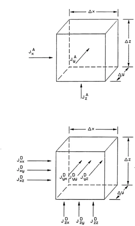
Table 3-1. Parameter Values For Analysis of Data from Rathbun and Tai (1988b)

Compound

(-)

Mi

(g/guiole)

Di He at 298 K

(cmVsxlO^) (—)

Benzene 0.606 78.11 10.9(2) 0.224('')

Toluene 0.598 92.14 9.5(2) 0.262('')

Ethylbenzene 0.595 106.17 9.0(2) 0.35 ('>

Ethylbenzene 0.586 106.17 9.0(2) 0.35 (5)

n-Propylbenzene 0.559 120.20 7.6(3) 0.44 (^)

n-Butylbenzene 0.535 134.22 7.0(3) 0.53 (5)

n-Butylbenzene 0.559 134.22 7.0(3) 0.53 (5)

n-Pentylbenzene 0.530 148.25 6.6(3) 0.65 (^> n-Hexylbenzene 0.475 162.28 6.2(3) 0.78 (^>

n-Heptylbenzene 0.411 176.30 5.8(3) 0.93 (^^

n-Octylbenzene 0.357 190.33 5.5(3) 1.10 (5)

(^) Experimental values determined by Rathbun and Tai (1988b).

(2) Experimental values compiled by Hayduk and Laudie (1974).

(3) Estimated using revised Othmer-Thakax equation (Hayduk and Laudie, 1974)

Di = 1.3 X io-4y-o-589

This is the same expression used by Rathbun and Tai.

(^) Experimental values from Leighton and Calo (1981)

(^) Estimated using expression from Rathbun and Tai (1988b) irc = 3.5 X 10-3V;„eO"°570Kn

where He [=] kPa-m3/gmole and the molar volume, V^ is

Fm = M./0.863 [=] ml/gmole

Values for the aqueous-phase difFusivities (£>/) and the Henry's constants (He) for the compovmds were obtained from existing experimental data and from pub¬

lished correlations. Table 3-1 presents the data used in the present analysis for the

compotmds. Rathbim and Tai used correlations to estimate all the diffusivities and

Rathbun and Tai used; for this reason, constants for the best-fit power correlation between mass transfer coefficient and diffusivity were recalculated for the present

analysis. The expression that Rathbun and Tai derived was

k}/kp ={5.65x10^ D^-^^^ (3-2)

As noted earlier in this section, neither this expression nor an expression using

molecular weights fit the experimental results over the entire range of the data. The expression derived here using the data in Table 3-1 was

ki/kf' = 476(D)°-"' (3-3)

Figure 3-1 is a plot of equation (3-3) and the experimental results. As in the expression developed by Rathbun and Tai, the correlation provided a poor fit to the

data. The sum of the squares of the errors (SSE) for the correlation was 1.7 x 10~^.

When the data were correlated with Henry's constant, the best fitting expression

was the following linear relationship

ki/kf' = 0.687 - 0.285Hc (3-4)

The SSE for this correlation was 2.4 x 10~^, about an order of magnitude less than

the error for the correlation given by equation (3-3) . A plot of the correlation and

the experimental results appears in Figure 3-2. Clearly, the linear correlation with Henry's constant provides a better fit to the data than does the power function correlation with diffusivity. One final correlation was developed. Optimal values

0.70

0.60

0.50

-o _

0.40

0.30

-0.20

1 1 > 1 1 1

- f~

)^<f'^^ o

o o ^^

o ^ ^^

—

o

. 0

-Frorfi Rathbun and

_{Tai (1988b)}

476D^-^^^'

E(Errors)^ = 1

1 . 1

.7x10"^

1

5.00 7.00 9.00 11.00

Liquid Diffusivity (cmVs x 10^)

ki/kf' = Ci + C2HC + C^D^* (3-5)

were determined. The resulting expression was

it;/jfcp^ =0.923-0.376Fc-520£>°-^^* (3-6)

Two points about equation (3-6) are noteworthy. The SSE for the correlation was the lowest of the three correlations at 1.2 x 10~^. In addition, the exponent on

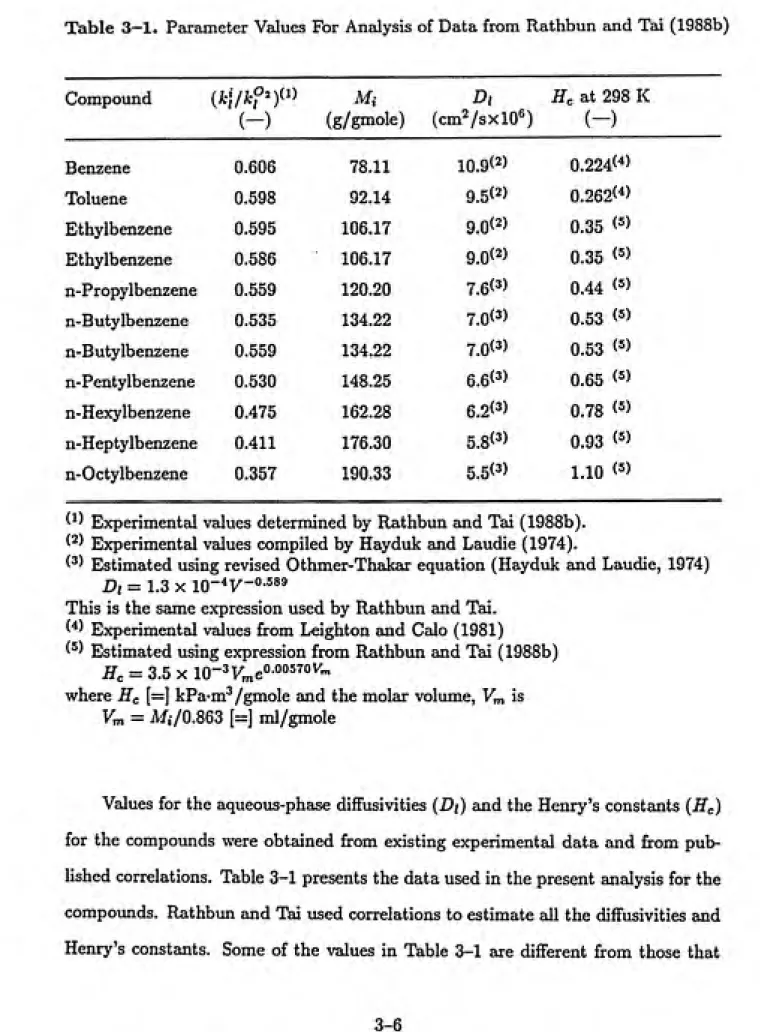
difFusivity is in agreement with boundary layer theory. Both these facts indicate that equation (3-6) is the best correlation for the data generated by Rathbun and Tai for the compounds benzene to n-octylbenzene. However, the negative coefficient on difFusivity in equation (3-6) leads to a contradiction with mass transfer theory: in this expression, k] decreases as difFusivity increases. Figure 3-3 is a plot of the

estimated values of fcj/fc^ ' vs the experimental values of k'^/kj ^ for equations (3-4) and (3-6) . Table 3-2 is a comparison of the experimental values with the values

obtained using the three correlations.

0.70

0.60

0.50

-O

^

0.40

0.30

-0.20

' 1 ' 1 '

- °v^

^

^^v o

^^\

--

ON^

Da Rathbun

ta From o .

and Tal (1988b)

- ooooo Experinnenta Va ues

k,'/kr = n 687 - n,?R5H

2(Erro

1

rsf = 2.4x10"^

1

0.00 0.40 0.80 1.20

Henry's Constant (dimenslonless)

c?

AAAAA 2(Error)^ =

ooooo SCError) =

o

(D

2.4x10 1.2x10

f^O.45

6X Data from

Rathbun and Tai (1988b)

AAAAA 0.687 - 0.285H

00000 0.923 - 0.376H - 520D

0.674

0.45 0.55 0.65

Experimental Value of k|'/k| ^

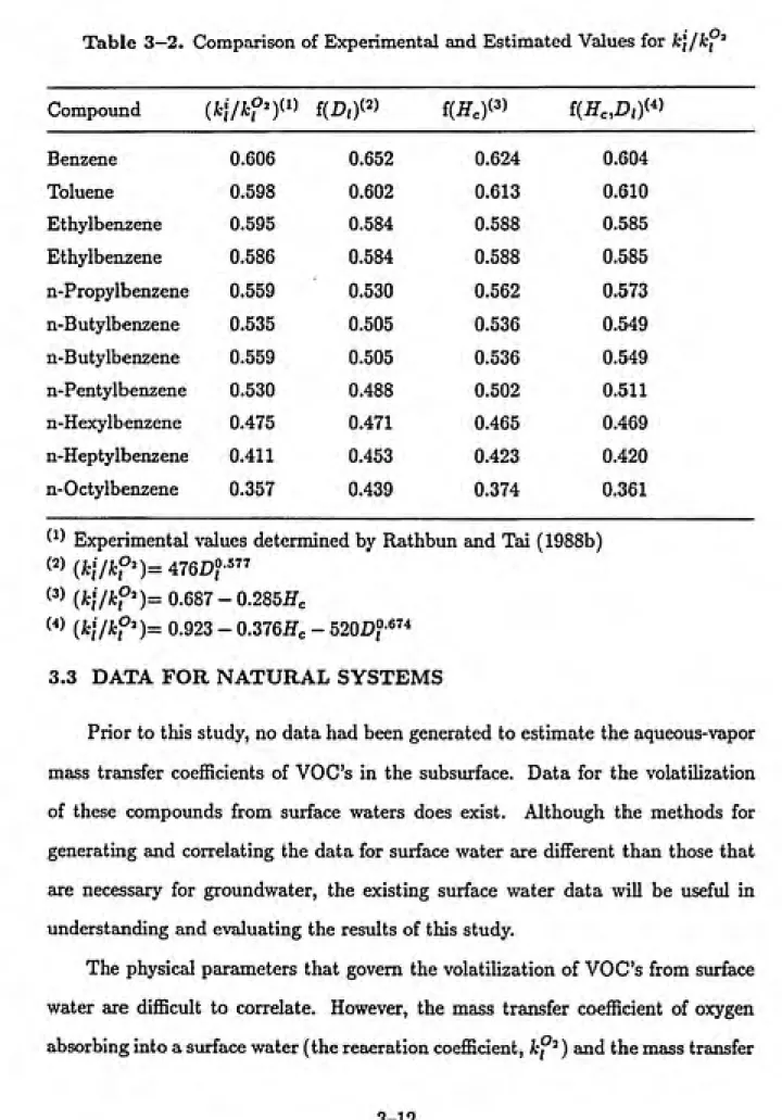
Table 3-2. Comparison of Experimental and Estimated Values for ArJ/fcf*^

Compound {k]ikf^r^ f(A)(^) f(^c)('^ i{Hc,Di)^'^

Benzene 0.606 0.652 0.624 0.604

Toluene 0.598 0.602 0.613 0.610

Ethylbenzene 0.595 0.584 0.588 0.585

Ethylbenzene 0.586 0.584 0.588 0.585

n-Propylbenzene 0.559 0.530 0.562 0.573

n-Butylbenzene 0.535 0.505 0.536 0.549

n-Butylbenzene 0.559 0.505 0.536 0.549

n-Pentylbenzene 0.530 0.488 0.502 0.511

n-Hexylbenzene 0.475 0.471 0.465 0.469

n-Heptylbenzene 0.411 0.453 0.423 0.420

n-Octylbenzene 0.357 0.439 0.374 0.361

(^^ Experimental values determined by Rathbun and Tai (1988b)

(2) (jfc;7jfcP^)=476D?"^ (3) {k\lkf^)= 0.687 - 0.285^c

(") {k\lkf')= 0.923 - 0.376ifc - 520D?-«^''

3.3 DATA FOR NATURAL SYSTEMS

Prior to this study, no data had been generated to estimate the aqueous-vapor

mass transfer coefficients of VOC's in the subsurface. Data for the volatilization

of these compounds from surface waters does exist. Although the methods for generating and correlating the data for surface water are different than those that axe necessary for groundwater, the existing surface water data will be useful in understanding and evaluating the results of this study.

The physical parameters that govern the volatilization of VOC's from surface water are difficult to correlate. However, the mass transfer coefficient of oxygen