1066.pdf

ABSTRACT

ROBERT H. GILBERTSEN. Application of contaminant fate and

transport models in saturated soil (Under the direction of

CASS T. MILLER.)

Systems that remediate an aquifer by purging

contaminated water often operate for prolonged periods

because contamination stubbornly lingers. This is the

tailing phenonmenon. For nondegradable, nonionic organics in

ground water, sorption is the prominent reaction. Sorption

is crucial to the tailing phenomenon.

Types of sorption rate expressions include (1) local

equilibrium, (2) Langmuir second order, (3) equilibrium/

first order, and (4) dual resistance sorption. Types of

equilibrium isotherms include (1) linear, (2) Freundlich, or

(3) Langmuir equilibrium.

This work improves four existing contaminant transport

simulator models; each model incorporates one sorption rate

assumption.

Based on modeling of the ground water contaminant nitro¬

benzene on Ann Arbor granular aquifer material in laboratory

librium models display the tailing phenomenon. The linear

TABLE OF CONTENTS

Page

LIST OF FIGURES... vi

LIST OF TABLES ... viii

ACKNOWLEDGEMENTS ... ix

I. INTRODUCTION ... 1

A. Ground water contamination, the general

problem ... 1

B. Contaminant tailing, the specific problem ... 2

C. Improved contaminant transport models, the

focus of this report ... 6

II. THEORETICAL BACKGROUND AND LITERATURE REVIEW --- 8

A. The advective-dispersive equation ... 9

B. The sorption expression ... 11

C. Related research ... 23

III. EXPERIMENTAL METHODS ... 25

A. Description of laboratory studies ... 25

B. Improvement of numerical models ... 26

C. Studies with the numerical models ... 36

IV. EXPERIMENTAL RESULTS AND DISCUSSION ... 39

A. Laboratory-scale analysis ... 39

V. CONCLUSIONS AND RECOMMENDATION ... 89

A. Conclusions ... 89

B. Recommendations ... 90

NOTATION...___ 91

REFERENCES ... 95

LIST OF FIGURES

Number

I-l

IV-1

IV-2

IV-3

IV-4

IV-5

IV-6

IV-7

IV-8

IV-9

IV-10

IV-11

IV-12

IV-13

IV-14

IV-15

IV-16

IV-17

IV-18

IV-19

IV-20

Page

The Tailing Phenomenon ... 5

LED Validation: Analytic Solution ... 40

LED Validation: Numerical Prediction ... 41

LSO Validation: Analytic Solution ... 42

LSO Validation: Numerical Prediction ... 43

FED Validation: Analytic Solution ... 44

FED Validation: Numerical Prediction ... 45

DUAL Validation: Analytic Solution ... 46

DUAL Validation: Numerical Prediction ... 47

Tracer Test 15-1 Fit with 21 Nodes ... 50

Tracer Test 16-1 Fit with 21 Nodes ... 51

Tracer Test 16-2 Fit with 21 Nodes ... 52

15-1, Linear LED, 1 Parameter Fit... 60

15-1, Freundlich LED, 1 Parameter Fit ... 61

15-1, LSO, 1 Parameter Fit ... 62

15-1, FED, 1 Parameter Fit... 63

15-1, DUAL, 1 Parameter Fit... 64

15-1, Linear LED, DH Sensitivity ... 68

15-1, Freundlich LED, DH Sensitivity ... 69

15-1, LSO, SOK Sensitivity ... 70

15-1, FED, Fast/Slow Sensitivity ... 71

IV-21 15-1, DUAL, FilltiK Sensitivity ... 72

IV-22 16-1, LSO, Predictive Mode ... 77

IV-23 16-1, FEL, Predictive Mode ... 78

IV-24 16-1, DUAL, Predictive Mode ... 79

IV-25 16-2, LSO, Predictive Mode ... 80

IV-26 16-2, FED, Predictive Mode ... 81

IV-27 16-2, DUAL, Predictive Mode ... 82

IV-28 Field Scale Simulation ... 88

LIST OF TABLES

Number Pacre

III-l Benchmark Testing in Various Computer

Environments ... 3 3

IV-1 Fitted Hydrodynamic Parameters ... 53

IV-2 Laboratory Column Parameters Known at Start

of Sorption Study ... 55

IV-3 Findings of Sorption Calibration Procedure ... 57

IV-4 Input Parameters for Models of Column 15-1,

the Calibration Run... 59

IV-5 Variance of Fitted Models of Column 15-1 ... 66

IV-6 Input Parameters for Models of Column 16-1,

A Predictive Run ... 75

IV-7 Input Parameters for Models of Column 16-2,

A Predictive Run ... 76

IV-8 Variance of Predictive Models of Column 16-1 . 83

IV-9 Variance of Predictive Models of Column 16-2 . 83

IV-10 Input Parameters for Field-Scale

Investigations ... 87

I would like to thank the citizens of North Carolina for

supporting my research through the Water Resources Research

Institute. Their grant titled "Modeling Organic Contaminant

Sorption Impacts on Aquifer Restoration" funded this

research.

I. INTRODUCTION

A. Ground water contamination, the general problem

Millions of Americans depend on ground water. At least

73 million people in the United States drink ground water

(JAWWA, 1986), or about one-third of the U.S. population.

This figure is not constant from state to state. Florida,

for instance, provides 90 percent of its residents with

drinking water from ground water (Tschinkel, 1986).

Because Americans depend so much on ground water, we

wish it were always safe and pure. Unfortunately this is

not the case. A great deal of ground water is contaminated.

A commonly quoted estimate of ground water contamination is

2 percent of the contents of U.S. aquifers, but even this

figure may underestimate the magnitude of the problem. The

National Research Council recently reviewed estimates of the

nation's ground water contamination. They dismissed earlier

claims that 2 percent of America's ground water is

contaminated as a "rough estimate based on oversimplified

assumptions." The Council believes that the actual level is

probably higher. Even if the percentage appears small, the

tendency for contamination to exist near population centers

contamination is the number of Superfund sites on the

National Priorities List. That number is now approaching

1000 and is expected to at least double (GWMR, 1985; SN,

1986; Grisham, et al., 1986). Presently there are 703

formal Superfund sites and 248 under consideration (USWN,

1987). EPA has no data on the volume of ground water

contaminated by these sites, but estimates that 75 percent

of the sites have produced observed ground water

contamination (ENR, 1986b).

Whatever the estimate of current contamination may be,

it is probably an underestimate. That is because a long lag

typically occurs between a contamination incident and the

eventual discovery of contamination. In ground water these

lags often stretch for decades. Even if people begin using

only safe waste disposal practices now, an increasing rate

of contaminant discovery will almost certainly continue

(Roberts et al.. 1982).

B. Contaminant tailing, the specific problem

After someone discovers that an aquifer is contaminated,

the land owner or the government often begins a cleanup

effort. Although a variety of cleanup options is available,

the most widely used option is the purge well method (Canter

and Knox, 1986). The concept of purge wells is simple. The

engineer deliberately places one or more withdrawal wells in

progresses over a period of time, the flow of water carries

away the contaminated water. The soil in the aquifer poses

a special problem because some contaminant sticks or "sorbs"

to the soil. This contaminated soil can continue to cause

problems by releasing sorbed contaminants even after wells

remove the the original contaminated water. In the purge

well method pure water does eventually wash even the

contaminated soil of the aquifer clean. Several

possibilities exist for disposing the withdrawn contaminated

water. Treatment and discharge to a surface water,

treatment and recharge to the ground water, and direct

discharge to sewers are typical disposal options.

Such cleanup operations can cost a great deal. The

average cost of cleaning up a Superfund site by whatever

method is about $8 million, but due to the great range of

aquifer and contaminant situations possible, that cost may

range from $200,000 to $2 billion (Kavanaugh, 1986). For

the specific case of well recovery systems, the single

greatest cost may be the energy cost of maintaining the

pumping for the years required to cleanse an aquifer (Canter

and Knox, 1986).

Given the high cost of cleaning contaminated aquifers in

general, and given the high energy cost of purge well

systems in particular, accurate prediction of contaminant

movement is crucial. Only by accurately understanding the

movement of a ground water contaminant plume can a ground

particular, accurate forecasts of cleanup time are vital to

economical design.

One drawback of many models currently in use, models

that couple the most commonly applied physical modeling

assumptions with the most commonly applied chemical modeling

assumptions, is the so-called "tailing" phenomenon (Roberts

et__al., 1982). In the field and even in the lab researchers

find that breakthrough response extends for considerably

longer than expected. It appears that the contaminant

sorbed to the soil takes longer to release than the

conventional model would predict. Figure I-l is an

illustrative example of what tailing might look like for a

purge well system. As the figure shows, at the start of

pumping the ground water is contaminated, but as pumping

progresses over time the ground water withdrawn becomes

FIGURE 1-1

THE TAILING PHENOMENON

z

O

I—

z UJ

o z

o

o

TS

D MEASURED VALUES

TIME

misleading forecast would incorporate grossly unrealistic

operation and maintenance costs. Since cleanup costs are

typically so large, this imprecision is important to

examine.

C. Improved contaminant transport models, the focus of

this report.

This work explores the hypothesis that the tailing

phenomenon results from a number of subtleties of

contaminant sorption. These subtleties are easily

understood, and mathematical modeling can anticipate them. A

discussion of two areas of concern follows.

First, most current ground water contaminant transport

models depend on the notion of instantaneous equilibration

of contaminant levels between the ground water and nearby

soil. This notion is generally based on batch reactor

experiments in which a small quantity of soil is stirred in

a solution of water containing a contaminant of interest.

The change in fluid phase contaminant concentration versus

contact time is customarily plotted in a graph. When this

measured change drops below experimental error, the system

is assumed to be at equilibrium. This approach is less than

rigorous, and may considerably underestimate the true time

required for attainment of equilibrium. That is because the

solid phase available for sorption comprises a nearly

activity may still occur in the solid without a noticeable

effect on the fluid phase. The conventional approach may

indicate that the system attains equilibrium within a few

hours when in fact, the equilibration process may continue

indefinitely (Coates and Elzerman, 1986).

Second, most current ground water contaminant transport

models hypothesize that the soil-water equilibrium isotherm

is linear. Recent work using low-organic soils over wide

ranges of contaminant concentration suggests that various

nonlinear isotherm models better define the equilibrium

condition (Miller and Weber, 1986).

This paper, then, is devoted to the improved modeling of

contaminant fate and transport by taking rate-controlled

kinetics, intraparticle diffusion, and nonlinear sorption

equilibrium into account. The technical report explores the

effect of rate-controlled kinetics, intraparticle diffusion,

and nonlinear sorption equilibrium on simulations of

laboratory soil columns and on simulations of a simple

field-scale application. Improvements of existing simulator

A. The advective-dispersive equation

The mathematical specification of physical and chemical

phenomena related to contaminant fate and transport makes

development of computerized, mathematical, ground-water

models possible. Such development begins here with the

fundamental physical processes — hydrodynamics — and then

adds the relevant chemical process — sorption.

Consider first an elemental volume. Within this unit

volume, conservation of mass dictates

Amass = area* (flux in) - area* (flux out) (H-l)

+(source or sink) + (reaction)

where

Amass = the net rate of change of contaminant mass within

the elemental volume (MT~ );

2

area = area of element face normal to velocity of flow (L );

— 2 —1

flux m = mass transfer into the elemental volume (ML T );

-2 -1

flux out = mass transfer from the elemental volume (ML T );

source or sink = contaminant mass added or removed (MT" );

The physical forces responsible for flux into and out of

the element are advection, mechanical dispersion, and

molecular diffusion. Most engineers assume Pick's law

governs mechanical dispersion and molecular diffusion. In

three dimensions, detailed consideration of mass balance

yields the advective-dispersive equation:

6C ^

— = - V • grade + div(Dj^gradC) (II-2)

5C ^b 6q

ͣ

^ (^-T^rxn -^ ^(C) + T (fit )srp

where

— 3

C = solution-phase solute concentration (ML );

t = time (T);

V = pore velocity vector (LT );

. . 2 —1

D, = second-rank hydrodynamic dispersion tensor (L T );

— 3 —1

V(C) = fluid-phase solute source (ML T );

—3

P, = bulk density of the soil phase (ML ) ;

6 = volume void fraction in the medium (dimensionless);

q = volume-average soil-phase mass normalized by the mass of

the solid phase (MM~ );

rxn = subscript denoting a general chemical or mass-transfer

reaction (dimensionless);

srp = subscript denoting sorption reaction (dimensionless).

This research considers the one-dimensional case. The

reduces to a simpler form in one-dimensional systems. In

one dimension without sources or sinks and without reactions

other than sorption, the mass-balance approach yields a

simpler equation. Physical chemists working with

chromatographic columns discovered this equation almost four

decades ago (adapted from Lapidus and Amundson, 1952):

6C 6C 6^C Pb (5g

^ = -^2 6^ + °h ^ - T ^^ ^srp (^^-3)

where

D, = longitudinal hydrodynamic dispersion coefficient

(L^t"^);

v_ = pore velocity in the longitudinal direction (LT~ );

2 = longitudinal distance variable (L).

Lapidus and Amundson performed their pioneering work in

ion exchange and chromatographic columns, but the basic

principles also apply to one-dimensional ground water flow

and ultimately to higher-dimensional, ground-water systems.

Interestingly, the chemists' early work examined the

relative applicability of rate and equilibrium controlled

sorption modeling, which is a central focus of this

technical report.

Although some researchers (van Genuchten, et al.. 1984;

11

Parker and Valocchi, 1986) argue that the

advective-dispersive equation presented here can oversimplify ground

water hydrodynamics, this research uses it for two reasons.

First, it is by far the most common means of analyzing

ground water fate and transport. Secondly, laboratory

tracer tests using a nonreactive, nonsorbing tracer suggest

that for the laboratory systems studied in this report the

advective-dispersive equation reasonably approximates the

hydrodynamics.

B. The sorption expression

Once system hydrodynamics are assumed, the only

remaining task in modeling the fate and transport of a

nondegradable contaminant is to specify the nature of the

sorption phenomenon. Because of the huge surface area over

which ground water and soil contact each other, accurate

characterization of sorption is indispensable to the

construction of a realistic ground-water

contaminant-transport model. Sorption is a general term used to

describe the uptake of a contaminant by soil without

specific reference to any particular mechanism. Sorption

encompasses both surface adsorption of a contaminant onto

the exterior of soil particles and also the partitioning of

a contaminant between water and the interior of soil

particles (Chiou, in press).

Considerable disagreement surrounds the sorption

equilibrium isotherm plots and the rate of equilibrium

attainment. The question of equilibrium isotherm shape

centers on whether increasing fluid-phase contaminant

concentration in the ground water causes a linear increase

in solid-phase contaminant concentration. The question of

rate centers on whether the contaminant in ground water

rapidly equilibrates with the contaminant sorbed in the soil

particles.

The next few pages detail the development of four

fundamentally different ways of looking at the sorption

expression. These formulations form the basis of the

computer programs revised for this research.

The local equilibrium approach

This approach (Freeze and Cherry, 1979) assumes that

interphase mass transfer occurs so rapidly that the solid

phase — the particles that compose the aquifer — and the

fluid phase — the ground water — are always in local

equilibrium.

Focusing specifically on the sorption term of equation

(II-3) and invoking the chain rule,

6q _ 6q 6C ^ (II-4)

&t 6C 6t

Equation (II-4) creates a need to define the relation

between the solid-phase concentration and the fluid-phase

13

equilibrium, the sorption isotherm provides the needed

information. One possible isotherm is the Freundlich

isotherm.

qe = Ve"" (^^-5)

where

q = equilibrium volume-average soil-phase mass normalized

by the solid-phase mass (MM~ );

rz Freundlich isotherm sorption-capacity constant

((lV^)");

K

C = equilibrium solution-phase concentration (ML~ );

n = Freundlich isotherm sorption-energy constant

(dimensionless).

Assuming local equilibrium, any solid-phase

concentration and fluid-phase concentration combination that

satisfies the equation is an equilibrium solution. This

permits differentiation of (II-5).

dq 5C

d3 = 6t "V • (^^-S)

Putting this new information to work, equation (II-4)

6q 6C n-1

6t = ^ "V • (^^-^)

Some researchers (Chiou, in press; Chiou, et_al., 1979;

Chiou, et al.. 1983) maintain that the Freundlich

coefficient equals unity for nonionic polar organics, the

class of contaminants of interest in this report. These

researchers suggest that nonionic polar organics sorb by

means of partitioning to the organic matter in aquifer

materials. In other words they believe that the sorption

isotherm is linear. This is also the conventional wisdom

among practicing engineers. Other researchers (Saltzman et

al.. 1972; Mingelgrin and Gerstl, 1983; and Miller and

Weber, 1986) claim that the Freundlich form with n not equal

to unity is more likely to be true, particularly in

low-organic aquifer materials over wide contaminant

concentration ranges. Such an extreme situation, they

maintain, is common in ground water, but rare in sorption

studies.

Regardless of whether the linear or nonlinear isotherm

is true, the derivative of the general Freundlich isotherm,

equation (II-7), may enter the advective dispersive

equation, equation (II-3) to yield

6C 6^C 6C ^b _ , 6C

15

Rearrangement yields

gC 6^C SC

where

Pb

,n-l

R^ = 1 + -g- nK-C /

R- = retardation factor.

The term Rf is the retardation factor. It has an

interesting property: If the Freundlich coefficient equals

unity the retardation factor is a constant. The constant

provides the ratio of the average ground water velocity to

the average contaminant velocity. This is a compelling

reason why engineers may wish to assume linear equilibrium,

quite apart from the question of whether the assumption of

linearity is rigorously true.

The Lanqmuir second-order approach

This model — which Hiester and Vermeulen (1952)

pioneered in packed-bed adsorbers — carries two

assumptions: (1) Sorption is a function of the product of

the fluid-phase concentration and the difference between the

sorption capacity and the contaminant concentration on the

solid phase. (2) Desorption is simply a function of the

Specifically, the solid-phase governing equation is

65 o ^

Tt = kg[C(Q° - q) - ^] (11-10)

where

Q° = Langinuir isotherm sorption-capacity constant (MM~ ) ;

3 —1 —1

k = second-order Langmuir model rate constant (L M T );

3 —1

b = Langmuir isotherm sorption-energy constant (L M ).

As conditions approach steady state, the above equation

yields the Langmuir isotherm.

*3e = 1 + bC • (11-11)

As before, this development is for a nondegradable,

nonreactive contaminant.

Substituting equation (11-10), the solid-phase governing

equation, into equation (II-3), the advective-dispersive

equation, yields

6C "S^c 6C

-^ = Dj^ -2 - V^ - (11-12)

'b q

17

Simultaneous solution of equation (11-12) and equation

(II- 10) links the solid-phase and fluid-phase solutions.

The first-order rate controlled with parallel ecfuilibrium

approach

Cameron and Klute (1977) were among the first to propose

this approach. It assumes that there are two types of sites

on the aquifer material where sorption may occur. The first

group of sites allows fast sorption. The model assumes

sorption there occurs so quickly that the fast sites locally

equilibrate with nearby ground water. At the second group

of sites sorption is slower. Sorption there proceeds

according to both rate and equilibrium expressions.

In equation form,

6q fi'^f ^%

where

q^ = volume-average soil-phase mass normalized by the mass

of the solid phase for the rapid sorption rate

component of the equilibrium/first-order model (MM~ );

q = volume-average soil-phase mass normalized by the mass

of the soild phase for the slow sorption rate component

of the equilibrium/first-order model (MM~ ).

Equation 11-14 is the solid-phase governing equation.

It is ready to substitute into equation (II-3), the

advective-dispersive equation. This yields

SC 6^0 6C ^b ^% gC 6'^s

5t = ^h —2 - ^z 5^ - r ^~C 6t + TT) • (^^-^5)

o z

Assuming that the Freundlich equilibrium model governs

the fast sites, equation (11-15) develops just as the

Freundlich local-equilibrium model did to produce

^F,f^fPb n--l 6C

(1 + —^---- ^ ) it (II-l^)

6^0 6c ^b ^%

" °h ^^2 " ^z 6^ -" "e" ~5t

where

Kp ^ = Freundlich isotherm sorption-capacity constant for

the rapid rate component of the

equilibrium/first-3 -1 &#equilibrium/first-34;f

order rate model ((L M ) );

n^ = Freundlich isotherm sorption-energy constant for the

rapid rate component of the equilibrium/first-order

rate model (dimensionless).

The addition of a first-order expression for the

19

6C S^C 5C '^b n

^f,f ^ = °h -2 - ^z 6^ - T "(^F,s C - ^s) (^^-17)

where

a = equilibrium/first-order mass-transfer coefficient (T~ );

R^ ^ = retardation factor for the rapidly sorbing fraction

in the equilibrium/first-order model (dimensionless);

K-, = Freundlich isotherm sorption-capacity constant for

r , s

the slow rate component of the

equilibrium/first-3 -1 &#equilibrium/first-34;s

order rate model ((L M ) );

n = Freundlich isotherm sorption-energy constant for the

Slow rate component of the equilibrium/first-order

model (dimensionless).

The slow-sorption solid-phase equation is

'^^ "s

"it = <^(^F,s'= - ^s) • (^^-IS)

simultaneous solution links equations (11-17) and (Il¬

ls).

The dual-resistance approach

Crittenden and Weber (1978) were among those who

performed early work with the dual-resistance model in

two-step process. For a molecule of contaminant to sorb to

the soil it must first pass through a film layer which

surrounds each soil particle and then diffuse into the soil

particle proper. Even though aquifer soil is mostly

impenetrable mineral, this does not detract from the model's

applicability. The diffusion process simply shifts to the

patches of organic matter which dot the exterior of the soil

particles, so the porous adsorbant model also applies to

sand grains as long as there is some organic matter on the

grains' exterior.

If the concentration of contaminant on a soil particle

composed of spherical shells equals the integral of

contaminant mass on each shell over the particle radius

divided by the particle volume, then

^ R 2

g = -^ ( .-^ r^g dr) (11-19)

_{R-^ •'o ^}

where

R = radius of soil particle (L);

r = radial distance variable for dual-resistance model (L);

q = solid-phase solute mass normalized by the mass of the

solid phase as a function of radial position (MM~ ),

21

t - „3 6t ( /_ ^ '^rdr) . (11-20)

6^ R-' '^^

ͣ

ͣ

'o

By applying a mass balance to mass transfer among

adjacent shells and assuming Fickian diffusion, the solid

phase governing equation is

2

6 Qj. 2 * "^r <5 ^s

°s (-2- + r T7) = Tt (1^-21)

_gr

where

D = intraparticle surface-diffusion coefficient for

dual-2 -1

resistance model (L T ).

The solid phase governing equation has two boundary

conditions. The first follows from radial symmetry at the

particle center.

(S r r=o

= 0 . (11-22)

The second combines Fickian diffusion at the films's

exterior with flux through the boundary-layer film.

a^r. I ^

f

where

kj = film mass transfer coefficient for the DUAL model

(LT"^);

C = fluid-phase, equilibrium-isotherm concentration

corresponding to the soil-phase concentration at the

—3

particle boundary (ML );

—3

p = density of the soil particle (ML ).

Although equation (11-20) defines the change of

solid-phase concentration with respect to time, a more practical

definition to substitute into the fluid-phase governing

equation comes from examination of flux.

^ = MASS FLUX * SURFACE AREA * particLE MASS ' ^^^'^^^

Substituting mathematical terms.

^ = kf(C - C3)*4TrR2* 4----3— . (11-25)

3 - ^ P

Simplification yields the change in the solid-phase

concentration with respect to time to plug into the

advective-dispersive equation.

6q 2^f(^ - ^s)

23

Now the advective-dispersive equation, equation (II-3)

becomes

6C 52^ 3 k^ (1 - e )

^ = °h 77---Ri---- (C - ^s) ' (1^-27)

which serves as the fluid-phase governing equation.

Simultaneous solution links the fluid-phase governing

equation, equation (11-27) with the solid-phase governing

equation, equation (11-21).

C. Related research

Valocchi (1985) examined the relative performance of

rate-controlled versus local-equilibrium-controlled sorption

in simulated one-dimensional ground water column

experiments. The study included not only chemical

nonequilibrium but also physical nonequilibrium models.

Valocchi did not examine the importance of isotherm shape

because he used the method of time moments, an analytical

analysis method that requires use of linear isotherms.

Chiou (in press) has conducted numerous batch laboratory

experiments to determine equilibrium sorption isotherm

shapes for a variety of nonionic organic solvents. His

studies have encompassed a range of organic matter content,

Miller (1984) studied and modeled sorption in batch

reactor laboratory systems and in laboratory soil column

reactors. His work included the contaminants lindane and

nitrobenzene, but focused on lindane. He demonstrated that

lindane exhibits nonlinear, rate-controlled sorption on

several granular aquifer materials.

This technical report is closely allied with the

original work of Miller. The chief distinctions of this

technical report are refinements of the numerical model

simulator programs and the modeling of the contaminant

III. EXPERIMENTAL METHODS

A. Description of laboratory studies

This technical report is an offshoot of the dissertation

of Miller (1984). All laboratory work and many programs

used in this technical report come from the work of Miller.

Clearly, a basic understanding of that work is a

prerequisite to understanding this work. This first section

of Chapter II provides a framework for such a basic

understanding. A reader interested in details should refer

to the original dissertation.

The original study is titled Modeling of Sorption and

Desorption Phenomena for Hydrophobic Organic Contaminants in

Saturated Soil Environments. The work consists of three

major parts: bottle-point equilibrium studies, completely

mixed batch reactor (CMBR) studies, and soil-column reactor

studies. It focuses on the sorption of two hydrophobic

organic contaminants taken one at a time on a variety of

glacially deposited Wisconsin Age sands.

Of particular pertinence to the present technical report

is the work on the contaminant nitrobenzene on Ann Arbor

soil. Miller's modeling thoroughly covers only bottle point

and CMBR reactors. The dissertation does not detail the

contaminant-soil combination even though a complete set of

laboratory data, rate parameters, and equilibrium parameters

is at hand.

Nitrobenzene (CgH_NO_), the contaminant used in the

experiments of interest, is also known as oil of mirbane.

It is a product of the organic chemical industry. Solvent

recovery plants use it, as do manufacturers of dyestuffs.

It is a solvent used in TNT production. It is also a

constituent in shoe polish. It has the odor of bitter

almonds. Miller studied it because of its common occurrence

in the environment, its moderately nonvolatile nature, its

resistance to degradation, and its partitioning properties.

The Ann Arbor soil had a median grain diameter of 0.232

mm, a grain size uniformity coefficient (dgQ/d^,.) of 2.616,

—3

a hydraulic conductivity of 4.15x10 cm/sec, a total

organic carbon content of 1.14 percent, and a cation

exchange capacity of 6.9 meq/lOOgr. Miller studied Ann

Arbor soil because of its sandy character, a character

shared my many aquifers tapped for potable water supplies.

This remainder of this chapter details how the student

used the infomnation from Miller's original studies,

modified and wrote computer programs, and then modeled

nitrobenzene on Ann Arbor soil in soil columns.

B. Improvement of numerical models

Computer model improvement represents by far the largest

27

At the start of this study, this research inherited four

FORTRAN computer programs which contained the basic

algorithms for finite difference solution of the four types

of sorption models presented in the previous chapter. The

programs were descendants of the programs Miller used in his

dissertation. These programs were named local equilibrium

with dispersion (LED); Langmuir second order sorption (LSO);

equilibrium / first-order sorption (FED); and

dual-resistance (DUAL).

The finite difference models are, of course, numerical

models, not analytical solutions. The nonlinearity of the

problems and the desire to have flexible control over

boundary conditions force the use of numerical models.

This paper often refers to five, not four models. That

is because the model LED does double duty. Depending on

whether the input data deck specifies linear isotherm

equilibrium or or Freundlich isotherm equilibrium, the model

operates under the name linear local equilibrium with

dispersion (L-LED) or Freundlich local equilibrium with

dispersion (F-LED).

The heart of each model is a set of governing finite

difference equations. These are spatially centered finite

difference approximations of the differential equations

presented in the previous chapter. The equations that

appear here are not the direct finite difference analogies

to the governing equations, but instead the "sorted"

dependent variable at like nodes appear together. DGEAR, an

IMSL subroutine, handles the time-stepping tasks. DGEAR is

a pre-packaged FORTRAN subroutine that solves differential

equations using Gear's method.

For LED the governing equation (II-8) becomes

^^i 1 ^h ^z 2 Dj^

f,l Az Az

Dh_ ^

ͣ

*" ^ ~2 " 2AZ ^ ^i+l^

Az

where

P

Rf^. = 1 + y nKp C."-l ,

i = column node index.

For each of the other models there are two governing

equations, a solid-phase and a fluid-phase equation. The

29

dC. D. V, 2D-

_{1 h z h}

dt " ^,2 "^ 2Az ^ ^i-1 "^ ^" .2 ^ ^i (III-2)

Az^ ^^

ͣ

"

ͣ

" Az

°h

"^ ^,,2 2Az^ *-^i+l

_AZ

^b _ ^i

sO

0

k3[(Q- - qi) C. -3]

The LSO solid phase equation (11-10) becomes

dq. q.

dt^ = k^[(Q° - qi) Ci - ~] . (III-3)

The FED fluid-phase equation (11-17) becomes

1 1 h z 1 h

~dt " r7T~ ^772 "^ 2A^^ ^i-1 "*" RTTT ^" 772^^i

_{f, f, 1 iiZ f, f, 1 Az}

^f,f,i ^Az2 " 2Az) ^i+l

Pj3 ^

The FED solid phase equation (11-18) becomes

^^s,i

-dt-= «(Kf,s ^i ' %,i^ ' (I^^-5)

The DUAL fluid-phase equation (11-27) becomes

dC ^h ^z ^°h 3k£(l-0)

dt " ^~[^ "^ TKi^ ^i-1 "^ ^~ ~^ " ^ ^ ^i

Dh ^z 3kf(l-e)

ͣ

•" ^"^ " 2Ai^ ^i+1 "^ ^ Re ^^s,i . (III-6)

The DUAL solid phase equation (11-21) becomes

D - ^ D

Ar, s D„ D„ s_^^

dq - s s +

^^ = ^ArAr_ " rAr^ *^r,l-l ^ ^" ArAr_ " ArAr^^ ^r,:

D^ D„

___^ __^

ͣ

•" ^ ArAr^ "^ rAr^ '3r,l+l (III-7)

where

31

Ar^ + Ar_

Ar =

---=---Ar =

Ar, =

^1 " ^1+1

^1+1 - ^1

+ 2

The changes to the existing programs follow.

1. Commenting of programs

The first change made to the four existing programs was

the addition of comment lines. These comment lines did not,

of course, affect the operation of the programs, but they

did improve the clarity of the programs. The task also

familiarized the student with the programs.

2. Transportability of programs

The second change was the conversion of the programs

from personal computer programs to a form that could easily

operate in either a mainframe or2 microcomputer environment.

The increased solution speed was a welcome improvement,

particularly for models such as DUAL which required many

hours to execute, even on a PC-AT. The needed changes

included restructuring of the program common blocks and

development of easily redirectable input and output units.

Several mainframe versions also ran on the Triangle

speed using the standard FORTRAN code developed for the

mainframe and microcomputer. Improved FPS-164 performance

would have required code specifically designed to take

advantage of the FPS-optimized library subroutines. Program

transportability took precedence over speed so further

programming efforts stayed in the mainframe and

microcomputer environments.

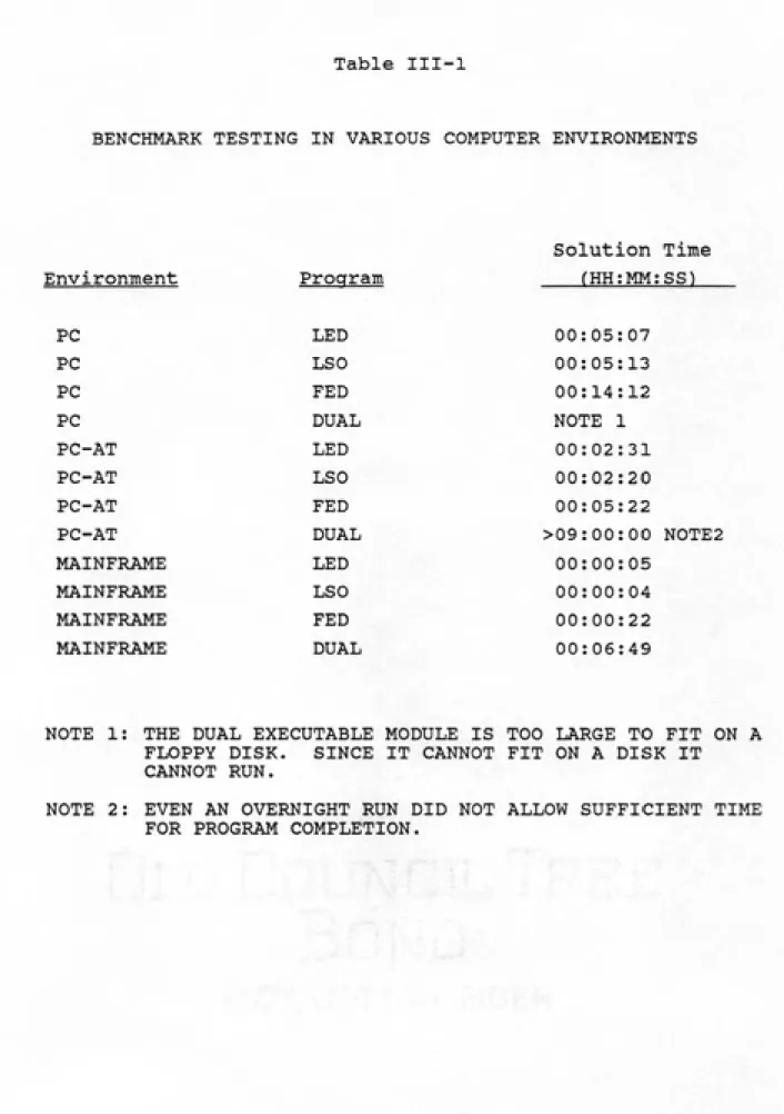
An early task performed to learn about the relative

usefulness of the various computer environments was

benchmark testing. Table III-l presents the performance of

a benchmark run in three different environments: the PC-AT,

an ordinary PC with a math coprocessor, and the mainframe.

The comparison attempted to isolate CPU time from

input/output time in order to report just the time spent

33

Table III-l

BENCHMARK TESTING IN VARIOUS COMPUTER ENVIRONMENTS

Environment

Procfram

Solution Time

fHH;MM;SS^

PC

PC

PC

PC

PC-AT

PC-AT

PC-AT

PC-AT

MAINFRAME

MAINFRAME

MAINFRAME

MAINFRAME

LED

LSO

FED

DUAL

LED

LSO

FED

DUAL

LED

LSO

FED

DUAL

00:05:07

00:05:13

00:14:12

NOTE 1

00:02:31

00:02:20

00:05:22

>09:00:00 N0TE2

00:00:05

00:00:04

00:00:22

00:06:49

NOTE 1: THE DUAL EXECUTABLE MODULE IS TOO LARGE TO FIT ON A

FLOPPY DISK. SINCE IT CANNOT FIT ON A DISK IT

CANNOT RUN.

NOTE 2: EVEN AN OVERNIGHT RUN DID NOT ALLOW SUFFICIENT TIME

3. Variation of influent

As the present research began, the computer simulation

models assumed constant soil column influent concentration.

The third change and the first major alteration of the

codes was the addition of variable influent concentration

capability. The modifications to the code allowed the

programs to accept both minor fluctuations in influent

concentration and drastic changes in influent concentration.

The user could now specify a constant influent concentration

or precisely steer the influent concentration. The

effluent boundary condition, the partial of concentration

with respect to location equals zero, remained unchanged.

The ability to control precisely the upstream boundary

condition was convenient when reproducing small experimental

fluctuations in the influent concentration. The control was

indispensable when studying sorption/desorption systems

where an elutriation phase follows a period of contaminant

feed.

A companion modification to the variable influent

provision was to add subroutines, INFOl and INF02, that

provide a detailed report of simulation status. As program

complexity increased the likelihood of blunders increased

dramatically. INFOl and INF02 helped to counteract this

natural tendency by displaying such relevant factors as

influent concentrations and the derivative of influent

35

programs were functioning properly, and to aid in

troubleshooting if they were not.

4. Variation of velocity

The fourth change was to accommodate a single update in

the soil column flow velocity at the time of contaminant

shutoff, should one occur. This was required because of a

peculiarity in the laboratory experimental design which

resulted in a change in contaminant velocity when

contaminant flow stopped and elutriation began.

5. Calculation of mass balance

The fifth and final change was the addition of an

automatic mass balance check. Numerical models, even ones

that are technically validated, always threaten an

unexpected numerical breakdown. These breakdowns were a

constant source of worry for the program operator since they

were not always obvious. Subroutines MASSl and MASS2

provided relief. The subroutines kept track of the

contaminant mass in the influent, contaminant mass in the

effluent, contaminant left in the soil, and contaminant left

in the fluid. By computing the ratio of input to accounted

mass at the end of each soil column simulation, these

subroutines assured the program operator that the

C. Studies with the numerical models

A six-step protocol for model development and

application drew ideas about the modeling process from a

paper by Thomann (1982).

MODEL DEVELOPMENT PROTOCOL

1. Formulate a model — a set of governing differential

equations plus boundary conditions — from consideration

of fundamental principles. Recast the model in terms of

a numerical scheme for solution.

2. Check the numerical model in an analytically tractable

scenario against an analytic solution. If it checks, the

model is technically validated.

3. Isolate and identify as many parameters as possible

through independent parameter determination.

4. Use an experimentally derived data set and force a fit

using parameters that could not be independently

established. Check that the parameters are plausible.

If the parameters are plausible and the prediction fits,

the model is calibrated, and operationally validated.

5. Take at least one more data set from a different set of

conditions and make a predictive run. If the prediction

fits the new data, the model is dynamically validated.

6. After every run perform a mass balance. This affords yet

another partial technical validation each time the model

37

Upon completion of the full set of activities from the

model development protocol at the lab scale, the research

returned to the original question of purge well analysis by

preparing an illustrative field-scale example.

Unfortunately, the lack of actual field-scale data prevented

application of the entire modeling process. The model was,

however, well suited to demonstrate the effect of the scale

of the problem on the prediction of the model.

The application of these modeling activities to Miller's

soil-column laboratory experiments and the illustrative

field scale model compose the subject matter of the next

A. Laboratory-scale analysis

This section details the results of the model

development protocol for the laboratory-scale analysis.

Technical validation precedes actual model use. One way

to make this validation is to compare predictions of the

numerical models against predictions of existing analytical

simulators from Miller (1984). When the predictions match,

it demonstrates that the central components of the numerical

models function correctly. Because this research uses

existing programs, the use of the technical validation is a

conservative approach.

The breakthrough curves produced in simplified,

analytically tractable situations follow in Figures IV-1

through IV-8. The curves appear in matched pairs that

present a numerical prediction and the corresponding

analytic prediction. The LED and FED predictions depict a

situation of contamination followed by elutriation. The LSO

FIGURE IV-1

0,9

0.8

z

o

1-

0,7

<

oc

t-z

_0.6

LU

o z

o

o

0.5

a

u

M

_0,4

-J

i

0,3

0.2

0,1

111 IIII mi mi in a

LED VALIDATION: ANALYTIC SOLUTION

wB)iiiiimi|HiiiniiiiiniiiiuiHiM«it

8

10

12

BED VOLUMES

2

O

1-<

ft: H 2

Ui

o

2

O o o

b!

-J

ft:

O

2

1

LEO VAUDATION:

NUMERICAL PREDICTION

r\ a

j^ 1 y-^

rv a

\

\

\

[3

\

1

\

I

\

1

\

n 1 _

J

\

U. 1

0 -

jDoe^

/

\

_^Qe*

3aDDaq3

8

10

12

z

o

I-z

Ul

o z

o o o

u

N

IT

O

z

1

0.9

0,8

0.7

0.6

0,5

0,4

0.3

0,2

0,1

FIGURE IV-3

LSO VALIDATION: ANALYTIC SOLUTION

.^^

.e--n

^

J^

y"

f^

^

ja

20

40

60

BED VOLUMES

LSO VALIDATION: NUMERICAL PREDICTION

<

I-z

o

O o

Q

Ui

M

o

z

0,9

0.8

0.7

0.6

0.5

0.4

0.3

0.2

0.1

r-r&

.^

^

ja13^

r

.y

^

3

-O0

y^

^^

ͣ

t-T

20

40

60

0,9

0.8

z

o

1—

0.7

<

a:

t-z

_0.6

o z

o

o

0.5

o

u

N

_0.4

1

fX.

_0.3

0.2

0.1

FIGURE IV~5

FED VALIDATION: ANALYTIC SOLUTION

i

^

\

/

\

/

\

/

_\

L J J

/

/

/

iiHiiiiiiinffIr'

/

Vb,

8

BED VOLUMES

o

I-<

o z

o

o

o

u

O

i _,

FED VAUDATION-

NUMERICAL PREDICTION

-. 1—It—» 1—1 !^-i f—ti—1#-^»—• •—I r—i •"*»-«—.

1

^^BO^ 1 p^

\

\

1

n "7

\

\

[ 3

\

I

t

_\

1

\

J

\

U. 1

r-i r—if*nr-i r

/

N

_'^^^^'^^ti

iDDaDct

0 —]

8

10

12

BED VOLUMES

FIGURE IV~7

DUAL VALIDATION: ANALYTIC SOLUTION

0.9

0.8

z

o

p

0.7

<

q:

1-2

_0,6

o

2

o

o

0.5

a

Ul

M

_0,4

~j

1

o

0.3

2

0.2

0,1

„«ee^

5&&°

^^^^l"~

^

^

/

V

^

/

y

20

40

60

DUAL VALIDATION: NUMERICAL PREDICTION

0,9

0.8

2 .

o

1-

0.7

<

CC

t-z

_0.6

o z

o

o

0.5

N

O

0.4

0.3

0.2

0.1

^^^ 1

„o-^

^^^

^

,^^

1

^

X

^

/

^

/^

/

\y

0

20

40

60

BED VOLUMES

ͣ

48

The analytic and numerical models match almost

perfectly; the models are technically validated.

The next step — isolation and independent estimation of

as many parameters as possible — begins with

characterization of system hydrodynamics. The system is a

suite of three soil column reactors packed with Ann Arbor

granular aquifer material. The operational names of these

columns are column 15-1, column 16-1, and column 16-2.

Miller's laboratory tracer tests conducted with the

chloride ion provide the means to characterize each column's

hydrodynamics. An automatic nonlinear parameter estimator

program attached to the front end of one of the improved

simulator programs (LED) drives the simulator. The

parameter estimator program uses the IMSL subroutine ZXSSQ.

ZXSSQ uses the Levenberg-Marquardt algorithm for nonlinear

optimization. The estimator drives the simulator, varying

only hydrodynamic dispersion until the sum of the squares of

the residuals of the model prediction with respect to the

observed data reach a minimum.

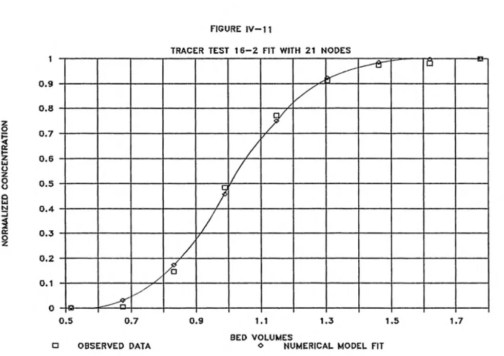
Limitations on the size of the DUAL program restrict

analysis to models with 21 column nodes, although for ideal

numerical model operation theoretical considerations would

call for as many as 3 6 column nodes. A comparison with a

theoretically more favorable situation not presented here

demonstrates that the consequences of the 21-node limitation

are minimal. Figures IV-9 through IV-ll illustrate the

Table IV-1 presents the optimal hydrodynamic dispersion

coefficient and dispersivity for each column as determined

by this research.

°h

where

a = longitudinal dispersivity (cm)

Dispersivity measures the tendency of the aquifer

material to cause dispersion and is independent of ground

FIGURE IV-g

z

o

o 2:

o

o

o

u N

tr

O

z

1

TRACER

TEST

15-1

FIT WITH 21

NODES

1

a

d

9

0 1

lJ,Tf

/

n "7 0, /

/

'

U.O

/

yjtA- —

/

rv 0

/

/

/

b

0 -

^

0.6

0.8

1,2

1.4

1.6

1.8

ͤ

OBSERVED DATA

BED VOLUMES

o NUMERICAL MODEL FIT

TRACER TEST 16-1 FIT WITH 21 NODES

0,9

0.8

z

o

1-

0.7

<

tc

V-z

_0.6

o

z

o

o

0.5

o

u

N

_0.4

-J

1

ct

_0.3

o

z

0.2

0,1

^

^^

—e-

I---1 n I---1

/

/

A

/

J

/

•t

/

/

/

ͣ

p -

.---E

^ei_

^^

0.1 0.3 0.5

ͤ

OBSERVED DATA

0.7

0.9

1.1

1.3

1.5

1.7

1,9

2.1

BED VOLUMES

FIGURE IV-11

TRACER TEST 16-2 FIT WITH 21 NODES

0,9

0.8

2

o

1—

0.7

<

ct H

2

_0.6

LU o

2 .•,

o

o

0.5

o

u

N

_0.4

Ui

i

a.

_0.3

^

0.2

0.1

.^-^

^^^-j""" ͣ'

ͣ

a---

,---B-]

/

/

V

/

y

A

-La---.

^-^"D

0.5

0.7

0.9

1.1

1.3

1.5

1.7

ͤ

OBSERVED DATA

BED VOLUMES

Table IV-1

Fitted Hydrodynamic Parameters

The table lists optimal hydrodynamic parameters for

columns modeled with 21 nodes.

Hydrodynamic

Dispersion Longitudinal

Column Coefficient Dispersitivity

Number (cm /hr) _____(cm)_____

15-1 2.22 0.453

16-1 1.86 0.587

54

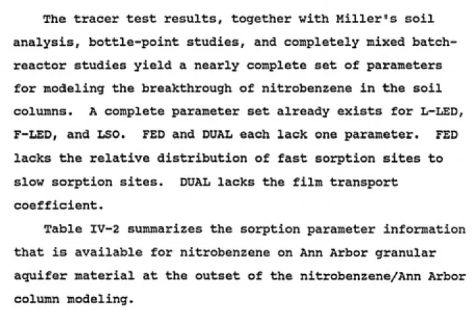
The tracer test results, together with Miller's soil

analysis, bottle-point studies, and completely mixed

batch-reactor studies yield a nearly complete set of parameters

for modeling the breakthrough of nitrobenzene in the soil

columns. A complete parameter set already exists for L-LED,

F-LED, and LSO. FED and DUAL each lack one parameter. FED

lacks the relative distribution of fast sorption sites to

slow sorption sites. DUAL lacks the film transport

coefficient.

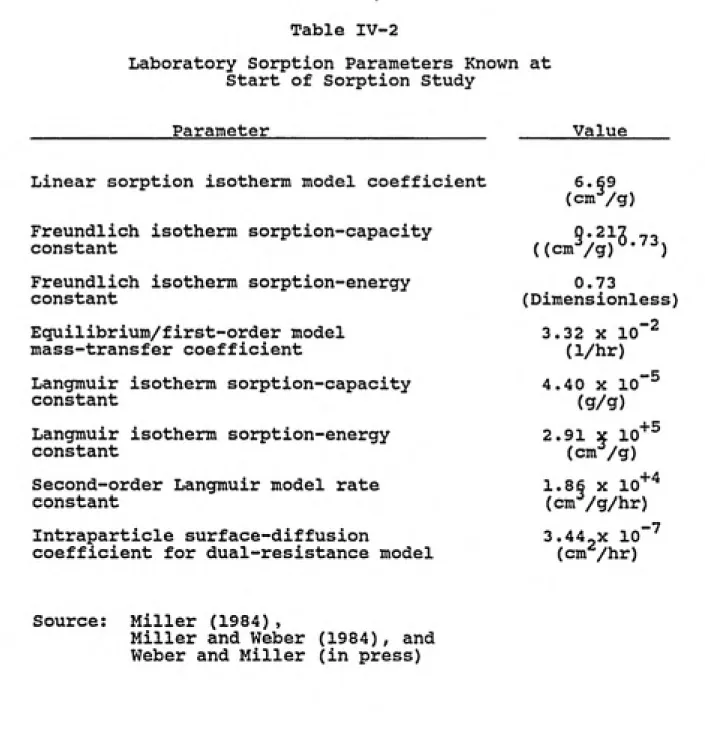
Table IV-2 summarizes the sorption parameter information

that is available for nitrobenzene on Ann Arbor granular

aquifer material at the outset of the nitrobenzene/Ann Arbor

Table IV-2

Laboratory Sorption Parameters Known at

Start of Sorption Study

Parameter

Value

Linear sorption isotherm model coefficient

Freundlich isotherm sorption-capacity

constant

Freundlich isotherm sorption-energy

constant

Equilibrium/first-order model

mass-transfer coefficient

Langmuir isotherm sorption-capacity

constant

Langmuir isotherm sorption-energy

constant

Second-order Langmuir model rate

constant

Intraparticle surface-diffusion

coefficient for dual-resistance model

6.69

(cm-^/g)

§•213 73

((cmVg)°-^^)

0.73

(Dimensionless)

.-2

32 X 10

(1/hr)

40 X 10

(g/g)

,91 X 10

(cmVg)

-5

+5

1.86 X 10"^'*

(cm /g/hr)

3.44-X 10"^

(cm'^/hr)

Source: Miller (1984),

56

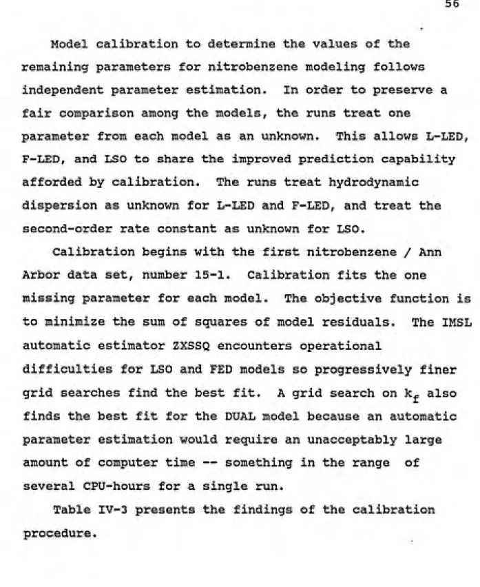
Model calibration to determine the values of the

remaining parameters for nitrobenzene modeling follows

independent parameter estimation. In order to preserve a

fair comparison among the models, the runs treat one

parameter from each model as an unknown. This allows L-LED,

F-LED, and LSO to share the improved prediction capability

afforded by calibration. The runs treat hydrodynamic

dispersion as unknown for L-LED and F-LED, and treat the

second-order rate constant as unknown for LSO.

Calibration begins with the first nitrobenzene / Ann

Arbor data set, number 15-1. Calibration fits the one

missing parameter for each model. The objective function is

to minimize the sum of squares of model residuals. The IMSL

automatic estimator ZXSSQ encounters operational

difficulties for LSO and FED models so progressively finer

grid searches find the best fit. A grid search on k^ also

finds the best fit for the DUAL model because an automatic

parameter estimation would require an unacceptably large

amount of computer time — something in the range of

several CPU-hours for a single run.

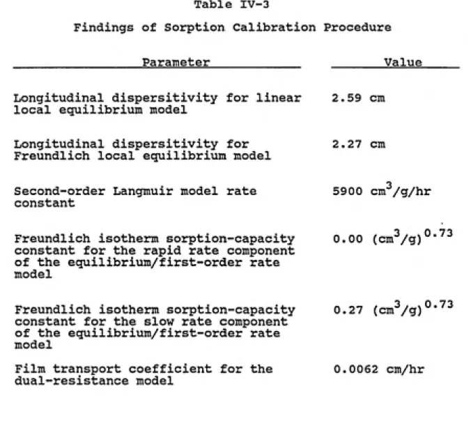
Table IV-3 presents the findings of the calibration

Table IV-3

Findings of Sorption Calibration Procedure

Parameter

Value

Longitudinal dispersitivity for linear 2.59 cm

local equilibrium model

Longitudinal dispersitivity for

Freundlich local equilibrium model

2.27 cm

Second-order Langmuir model rate

constant

5900 cm /g/hr

Freundlich isotherm sorption-capacity

constant for the rapid rate component

of the equilibrium/first-order rate

model

0.00 (cm^/g)°''^^

Freundlich isotherm sorption-capacity

constant for the slow rate component

of the equilibrium/first-order rate

model

Film transport coefficient for the

dual-resistance model

0.27 (cmVg)°'^"^

58

Comparison of Table IV-2 with Table IV-3 provides

favorable information: For the three models where parameter

estimation is not absolutely necessary, the parameter values

do not shift dramatically.

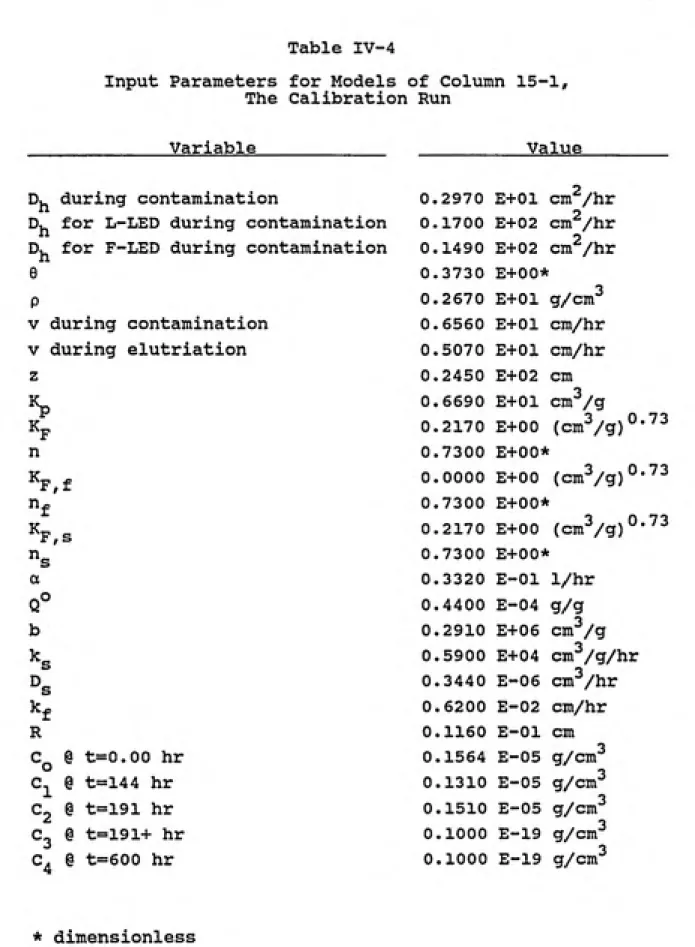
Plotting the model predictions for column 15-1 along

with the experimental breakthrough measurements provides

means to assess whether the calibrations are successful.

Table IV-4 presents the input parameters for each model.

Table IV-4

Input Parameters for Models of Column 15-1,

The Calibration Run

Variable

Value

Dv^ during contamination

Dy^ for L-LED during contamination

D, for F-LED during contamination

e

V during contamination

V during elutriation

n

K.

K

a

b

k

F,f

F,s

s

R

C,

@ t=0.00 hr

@ t=144 hr

@ t=191 hr

@ t=191+ hr

@ t=600 hr

0.2970 E+01 cm /hr

0.1700 E+02 cm^/hr

0.1490 E+02 cm^/hr

0.3730 E+00*

0.2 670 E+01 g/cm^

0.6560 E+01 cm/hr

0.5070 E+01 cm/hr

0.2450 E+02 cm

0.6690 E+01 cm-^/g

0.2170 E+00 (cm-^/g)°"'^^

0.7300 E+00*

0.0000 E+00 (cm-^/g)°*^-^

0.7300 E+00*

0.2170 E+00 (cm-^/g)^''^-^

0.7300 E+00*

0.3320 E-01 1/hr

0.4400 E-04 g/g

0.2910 E+06 cm^^/g

0.5900 E+04 cm-^/g/hr

0.3440 E-06 cm-^/hr

0.6200 E-02 cm/hr

0.1160 E-01 cm

0.1564 E-05 g/cm"^

0.1310 E-05 <3/ctP

0.1510 E-05 g/cm^^

0.1000 E-19 g/cm'^

0.1000 E-19 g/cm-^

FIGURE IV~12

15-1, LINEAR LED, 1 PARAMETER FIT

z

o

I-2

Ui

o z

o

o

a

u

N

o

z

20

40

60

80

100

120

ͤ

OBSERVED DATA

BED VOLUMES

o NUMERICAL MODEL FIT

15-1, FREUNDLICH LED, 1 PARAMETER FIT

0.9

0.8

2:

F

0.7

<

oc

Y-z

_0.6

Ul

0

z

0

0

0.5

0

u

N

_0.4

t

fX.

_0.3

0

z

0,2

0.1

/

20

40

60

80

100

120

ͤ

OBSERVED DATA

BED VOLUMES