Parallel Implementation of Desirability Function-Based Scalarization
Approach for Multiobjective Optimization Problems
O. Tolga Altinoz
Ankara University, Electrical and Electronics Engineering, Turkey E-mail: [email protected]
Eren Akca
HAVELSAN A.S., Ankara, Turkey E-mail: [email protected]
A. Egemen Yilmaz
Ankara University, Electrical and Electronics Engineering, Turkey E-mail: [email protected]
Anton Duca and Gabriela Ciuprina
Politehnica University of Bucharest, Romania E-mail: [email protected], [email protected]
Keywords:parallel implementation, CUDA, particle swarm optimization
Received:December 1, 2014
Scalarization approaches are the simplest methods for solving the multiobjective problems. The idea of scalarization is based on decomposition of multiobjective problems into single objective sub-problems. Every one of these sub-problems can be solved in a parallel manner since they are independent with each other. Hence, as a scalarization approach, systematically modification on the desirability levels of the objective values of multiobjective problems can be employed for solving these problems. In this study, de-sirability function-based scalarization approach is converted into parallel algorithm and applied into seven benchmark problems. The performance of parallel algorithm with respect to sequential one is evaluated based on execution time on different graphical processing units and central processing units. The results show that even the accuracy of parallel and sequential codes are same, the execution time of parallel algo-rithm is up to 24.5-times faster than the sequential algoalgo-rithm (8.25-times faster on average) with respect to the complexity of the problem.
Povzetek: Pristopi s skalarizacijo sodijo med najenostavnejše naˇcine reševanja veˇckriterijskih problemov. Zamisel skalarizacije temelji na dekompoziciji veˇckriterijskih problemov v enokriterijske podprobleme, ki jih lahko rešujemo soˇcasno, saj niso medsebojno odvisni. Torej lahko uporabimo za reševanje veˇckriteri-jskih problemov sistematiˇcno spreminjanje nivoja zaželenosti ciljnih vrednosti teh problemov. V tej študiji smo implementirali vzporedni naˇcin skalarizacije na osnovi funkcije zaželenosti in ga aplicirali na sedmih tesnih problemih. Uˇcinek vzporednega algoritma glede na zaporednega smo ovrednotili z ozirom na ˇcas izvajanja na razliˇcnih grafiˇcno-procesnih in centralno-procesnih enotah. Vzporedna razliˇcica daje enako natanˇcne rezultate in je tudi do 24,5-krat hitrejša od zaporedne (8,25-krat v povpreˇcju), glede na zahtevnost problema.
1
Introduction
The problem for determining the best possible solution set with respect to multiple objectives is referred to as a multi-objective (MO) optimization problem. There are many ap-proaches for the solution of these kinds of problems. The most straightforward approach, the so-called “scalariza-tion” or “aggrega“scalariza-tion” is nothing but to combine the ob-jectives in order to obtain a single-objective [1].
computa-doned due to the necessary of much higher number of func-tion evaluafunc-tions to obtain approximately same performance as multiobjective optimization algorithms. However, with the aid of parallel architectures and devices, it is possible to reconsider and revisit the scalarization techniques since these techniques are usually suitable for parallelization.
One of the scalarization approaches for a-priori process is defined with the aid of a desirability function in this study. Desirability function is integrated to the particle swarm optimization algorithm in order to normalize the joint objective function values [5]. Then, geometric mean of the desirability levels of each objective is computed in order to obtain a single value. For each sub-problem, the shape of the desirability function is shrunk. Therefore the desirability level is changed and the optimization re-sults are also varied. At the end of this method, a set of possible solutions are composed. This set contains both the dominated and the non-dominated solutions. If nec-essary, the programmer might run a posterior method like non-dominated sorting for selecting the non-dominated so-lutions, as well. However, in this study, the main focus is to obtain the possible solution set. In this study, with a similar motivation, we demonstrate how one of these techniques can be parallelized and present performance of the approach by implementing on the Graphic Processing Units (GPUs) via the Compute Unified Device Architec-ture (CUDA) framework.
This paper is organized as follows: Section 2 explains the desirability function-based scalarization approach in detail and Section 3 presents a parallel implementation of the proposed method. Section 4 gives the implementation environment, benchmark problems and performance evalu-ation of the proposed method. The last section presents the conclusion and future work off the proposed method.
2
Desirability Function-Based
Scalarization Approach
In a general manner, the desirability functions can be ap-plied in order to incorporate the decision maker’s prefer-ences without any modification of the single-objective op-timization algorithm. The decision maker chooses a
desir-that proposed method is applied as a scalarization approach like weighted sum method. Therefore a systematic ap-proach was previously proposed by changing the shape of desirability functions by three of the authors of this paper [6]. ForN objective problem,N numbers of desirability functions are selected with respect to the boundaries of the problem. Next, desirability functions are divided into lev-els and each level corresponding to one of the single objec-tive implementation. For example of two objecobjec-tive problem case which was investigated in this paper, two desirability functions are defined and they are divided into same level (let’s say 10) per function. Since there are two desirabil-ity functions defined, there are 100 single objective imple-mentations in total. The previous study [6] show that the performance of the desirability function is greatly depends on the number of the levels, in other words the number of the single objective evaluations. Also the results obtained in the previous study are showed that, it is acceptable for bi-objective problems. However, still the performance of the proposed approach is greatly depends on the number of levels, which increases the total number of computation time. Hence, in this study, the parallel cores of CPU and GPU are using as computation units for single objective optimization algorithms, and the total evaluation times are recorded for comparison. The aim of this paper is to show the applicability of the proposed method with the aid of parallel architectures of CPU and GPU.
2.1
Desirability Function
The desirability function idea was first introduced by Har-rington in 1965 for the multi-objective industry quality control. After the proposition of the desirability function concept, Deringer and Suich [7] introduced two different desirability function formulations, which become the fun-damental equations of desirability functions. These two de-sirability function definitions are given by (1), (2) and (3), which are called one-sided and two-sided, respectively.
The parameters given in equations are as follows: y is the input, for our case it is the objective function value,
hmin,hmaxandhmedare the minimum, maximum and the
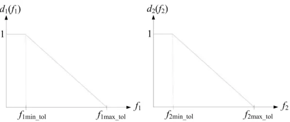
Figure 2: The linear desirability functions constructed for the bi-objective optimization problem.
d1(y) =
1, y < hmin
( y−hmax
hmin−hmax)
r, h
min< y < hmax
0, y > hmax
(1)
d2(y) =
0, y < hmin
( y−hmin
hmax−hmin)
r, h
min< y < hmax
1, y > hmax
(2)
d3(y) =
0, y < hmin
( y−hmin
hmed−hmin)
t, h
min< y < hmed
( y−hmax
hmed−hmax)
s, h
med< y < hmax
0, y > hmax
(3)
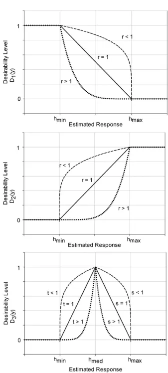
The desirability leveld(y) = 1is the state for fully desir-able, andd(y) = 0is for a not-desired case. In this respect,
d1 one-sided desirability function is useful for
minimiza-tion problem. The curve parameters arer,tands. They are used in order to plot an arc instead of solid line, when desired. Curves plot in Figure 1 demonstrate the effects of the curve parameters and the graphs of the desirability functions.
2.2
Method of Desirability Function-Based
Scalarization
The main idea beneath the desirability functions is as fol-lows:
– The desirability function is a mapping from the do-main of real numbers to the range set[0,1].
– The domain of each desirability function is one of the objective functions; and it maps the values of the rel-evant objective function to the interval[0,1].
– Depending on the desire about minimization of each objective function (i.e., the minimum / maximum tol-erable values), the relevant desirability function is constructed.
– The overall desirability value is defined as the geomet-ric mean of all desirability functions; this value is to be maximized.
Particularly, for a bi-objective optimization problem in which the functions f1 andf2 are to be minimized, the
relevant desirability functions d1(f1) and d2(f2) can be
defined as in Figure 2. The desirability functions are not necessarily defined to be linear; certainly, non-linear defi-nitions shall also be made as described in [7].
Throughout this study, we prefer the linear desirability functions.
In [6], a method for extraction of the Pareto front was proposed by altering the shapes of the desirability functions in a systematical manner. Particularly by:
– Fixing the parameters f1max_tol andf2max_tol seen in
Figure 2 at infinity, and
– Varying the parametersf1min_tol andf2min_tol
system-atically,
It is possible to find the Pareto front regardless of its con-vexity or concavity. This claim can be illustrated for the bi-objective case as follows: as seen in Figure 3, the param-eters f1min_tol and f2min_tol determine the sector which is
traced throughout the solution. The obtained solution cor-responds to a point for which the geometric mean of the two desirability values. As seen in Figure 4, even in the case of concave Pareto front, the solution can be found without loss of generality. In other words, unlike the weighted-sum approach, the method proposed in [6] does not suffer from the concave Pareto fronts.
Figure 1: The graphical demonstration of the desirability functions.
Figure 4: The solution via the desirability-function based approach for concave Pareto front.
solved with Particle Swarm Optimization. Despite no ex-plicit demonstration or proof, it was claimed that:
– There were no limitations about the usage of Parti-cle Swarm Optimization; i.e., any other heuristic al-gorithm could be incorporated and implemented.
– The proposed method can be easily parallelizable.
In this study, we demonstrate the validity of these claims by performing a parallel implementation on GPUs via the CUDA framework. The next section is devoted to the im-plementation details.
3
Parallel Multiobjective
Optimization with GPU
This section is dedicated to explaining the steps and idea of parallelizing the Desirability function-based scalarization approach with the aid of CUDA library.
3.1
Fundamentals of CUDA Parallel
Implementation
be converted to a parallel kernel by using the libraries and some prefix expressions. By this way, the programmers do not need to learn a new programming language. They are able to use their previous know-how related to C/C++, and enhance this knowledge with some basic expressions intro-duced by CUDA. However, without the knowledge about the CUDA software and the parallel architecture hardware, it is not possible to write efficient codes.
CUDA programming begins with the division of the ar-chitectures. It defines the CPU as host and GPU as de-vice. The parallel programming actually is the assignment of duties to parallel structure and collection of the results by CPU. In summary, the codes are written for CPU on C/C++ environment, and these codes include some paral-lel structures. These codes are executed by the host. Host commands device for code executed. When the code is exe-cuted by the device, the host waits until the job is finished, then a new parallel duty can be assigned, or results from the finished job can be collected by the host. Thus, the de-vice becomes a parallel computation unit. Hence, parallel computing relies on the data movement between host and device. Eventhough both host and device are very fast com-putation units, the data bus is slower. Therefore, in order to write an efficient program, the programmer must keep his/her code for minimum data transfer between the host and the device.
The GPU has stream multiprocessors (SMs). Each SM has 8 stream processors (SPs), also known as cores, and each core has a number of threads. In tesla architecture there are 240 SPs, and on each SP has 128 threads, which is the kernel execution unit. The bodies of threads are called groups. The groups are performed collaterally with respect to the core size. If the GPU architecture has two cores, then two blocks of threads are executed simultaneously. If it has four cores, then four blocks are executed collaterally.
Host and device communicate via data movement. The host moves data to the memory of the GPU board. This memory is called global memory which is accessed from all threads and the host. The host has also access to con-stant and texture memories. However, it cannot access the shared memory, which is a divided structure assigned for every block. The threads within the block can access their own shared memory. The communication of the shared memory is faster than the global memory. Hence, a par-allel code must contain data transfers to shared memory more often, instead of global memory.
In this study, random numbers are needed to execute the algorithm. Hence, instead of the rand() function of the C/C++ environment, CURAND library of the CUDA pack has been employed. In addition, the CUDA Event is pre-ferred for accurate measurement of the execution time. In the next section, the parallel implementation of desirability function-based scalarization was explained in detailed.
3.2
Parallel Implementation of Desirability
Function-Based Scalarization
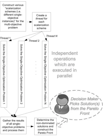
The main idea of our parallel implementation throughout this study is illustrated in Figure 5.
Each scalarization scheme is handled in a separate thread; after the relevant solutions are obtained, they are gathered in a centralized manner to constitute the Pareto front from which the human decision maker picks a solu-tion according to his/her needs. This approach ensures that the number of solutions found that can be found in parallel is limited by the capability of the GPU card used.
As stated before, we implemented the Particle Swarm Optimization Algorithm for verification of the aforemen-tioned claims. The parallel CUDA implementation was compared to the sequential implementation on various GPUs and CPUs.
Figure 5: The parallel CUDA implementation of the desirability-function based approach.
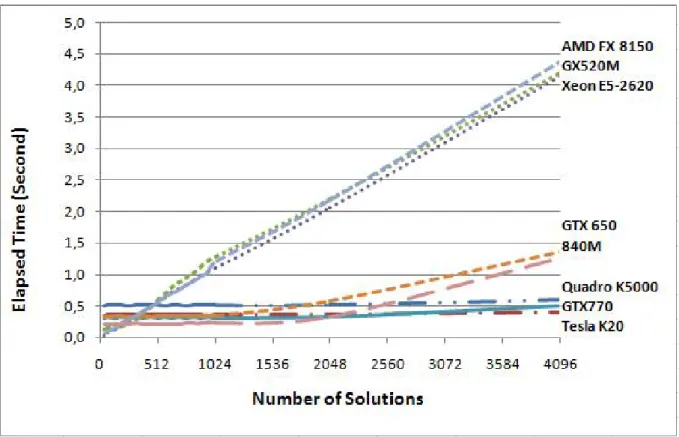
It was seen that both implementations (sequential and parallel CUDA) were able to find the same solutions but in different elapsed times. As seen in Figure 6, if the num-ber of Pareto front solutions increase, the advantage of the parallel CUDA increases dramatically.
– An old-fashion mobile GPU performs almost same as a relatively high level CPU.
– As the number of solution increases, the professional high level GPU devices perform more stable than gen-eral purpose GPUs.
4
Implementation, Results, and
Discussion
The parallel desirability function-based scalarization ap-proach was applied to solve seven benchmark problems. These problems are selected based on the complexity against execution time on computation unit. Since the av-erage number of execution time is considered in the study, problems from simple calculation to problems with more branch and complex functions. In this section the bench-mark problems and the results with respect to execution time is presented.
4.1
Benchmark Problems
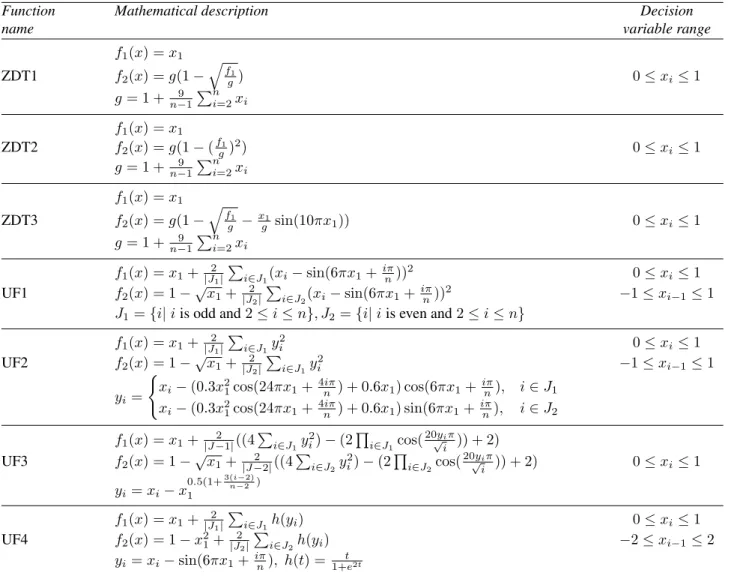
In this study, ten benchmark problems [9] with different complexity and Pareto shape are selected to present the per-formance of the method. Table 1 gives the mathematical formulations of the problems. The performance compar-ison is performed not only on the accuracy of the results, but more importantly on the execution time. As given in Ta-ble 1 the complexity of the benchmark proTa-blems are given from simple to more complex problems. The reason be-hind is that as the complexity of the function is increased, the single processors have to accomplish much more cal-culations, and since the single processors on a GPU has lower capacity than CPU, it will be a good comparison for not only the number of solutions in solution space but also the problem complexity.
Table 1 presents as three columns. The first column gives the known-names of benchmark problems. The reader can be access amount of information about the function by searching by selecting keyword as function name. The sec-ond column is the mathematical formulation of the func-tion. As the order of row increases the complexity of the
cutions earlier than GPU. From 400 to6,400levels, GPU computation time of parallel codes exceeds CPU time. At 6,400 levels, the difference between CPU and GPU is at the peak grade. After that level, the advantage of GPU re-duces. In other words, the GPU implementation acts more sequentially, since there are not any empty resources to ex-ecute parallel implementation. Among all of the problems, UF1 is the hardest for GPU implementation since the com-putation time is the longest for this problem. The main reasons are that: a) checking mechanism for even and odd parts that adds branch to the code, b) square of the trigono-metric function. for GPU implementation branch are the time consuming programming codes such that in an if-else, both parts are evaluated by the architecture, that reduces the resources.
The average execution time of CPU is 8.25-times slower than average GPU execution time. The following results are obtained for comparison the execution time:
– For a small number of solutions, CPU outperforms GPU
– The increase on CPU execution time is proportional to the number of solutions. Hence, the execution time on CPU increases.
– The GPU implementations are much beneficial for overall comparison.
– For a very high number of solutions, the improve-ments obtained in GPU slowly decreases since GPU contains limited number of stream (multi)processors. At some point the improvements are not lower than≈ 10-times on average.
5
Conclusion
Table 1: Multiobjective benchmark problems
Function Mathematical description Decision
name variable range
f1(x) =x1
ZDT1 f2(x) =g(1− qf
1
g) 0≤xi≤1
g= 1 + n−91Pn
i=2xi
f1(x) =x1
ZDT2 f2(x) =g(1−(fg1)2) 0≤xi≤1
g= 1 + n−91Pn i=2xi
f1(x) =x1
ZDT3 f2(x) =g(1− q
f1
g − x1
g sin(10πx1)) 0≤xi≤1
g= 1 + 9
n−1 Pn
i=2xi
f1(x) =x1+|J21|Pi∈J1(xi−sin(6πx1+
iπ n))
2 0≤x
i≤1
UF1 f2(x) = 1−
√
x1+|J2 2|
P
i∈J2(xi−sin(6πx1+
iπ n))
2 −1≤x
i−1≤1
J1={i|iis odd and2≤i≤n}, J2={i|iis even and2≤i≤n}
f1(x) =x1+|J21|Pi∈J1y 2
i 0≤xi≤1
UF2 f2(x) = 1−
√
x1+|J2 2|
P
i∈J1y 2
i −1≤xi−1≤1
yi=
(
xi−(0.3x21cos(24πx1+4niπ) + 0.6x1) cos(6πx1+iπn), i∈J1
xi−(0.3x21cos(24πx1+4niπ) + 0.6x1) sin(6πx1+iπn), i∈J2
f1(x) =x1+|J−21|((4Pi∈J1y 2
i)−(2
Q
i∈J1cos( 20√yiπ
i )) + 2)
UF3 f2(x) = 1−
√
x1+|J−22|((4
P
i∈J2y 2
i)−(2
Q
i∈J2cos( 20√yiπ
i )) + 2) 0≤xi≤1
yi=xi−x
0.5(1+3(n−i−22)) 1
f1(x) =x1+|J2 1|
P
i∈J1h(yi) 0≤xi≤1
UF4 f2(x) = 1−x21+|J22| P
i∈J2h(yi) −2≤xi−1≤2
impr 0.3072 0.2420 0.3934 0.2237 0.2242 0.2222 0.2304 0.2633
CPU 0.221 0.153 0.291 0.222 0.199 0.197 0.168 0.2073
10×10 GPU 0.439 0.451 0.4848 0.4934 0.49 0.4914 0.405 0.4649
impr 0.5034 0.3392 0.6002 0.4499 0.4061 0.4009 0.4148 0.4450
CPU 0.446 0.333 0.576 0.42 0.418 0.413 0.372 0.4254
15×15 GPU 0.4424 0.4576 0.4904 0.499 0.4944 0.4967 0.409 0.4699
impr 1.0081 0.7277 1.1746 0.8417 0.8455 0.8315 0.9095 0.9055
CPU 0.8 0.564 0.997 0.717 0.706 0.728 0.811 0.7604
20×20 GPU 0.4281 0.442 0.4781 0.5 0.4977 0.5 0.4146 0.4658
impr 1.8687 1.2760 2.0853 1.4340 1.4185 1.4560 1.9561 1.6421
CPU 1.21 0.893 1.521 1.12 1.444 1.114 0.987 1.1841
25×25 GPU 0.4393 0.4573 0.491 0.5 0.4954 0.499 0.408 0.4700
impr 2.7544 1.9528 3.0978 2.2400 2.9148 2.2325 2.4191 2.5159
CPU 1.753 1.266 2.279 1.582 1.589 1.59 1.428 1.6410
30×30 GPU 0.4424 0.4566 0.4871 0.501 0.4973 0.4979 0.4132 0.4708
impr 3.9625 2.7727 4.6787 3.1577 3.1953 3.1934 3.4560 3.4880
CPU 3.162 2.186 4.094 2.794 2.854 2.757 2.508 2.9079
40×40 GPU 0.4451 0.453 0.4893 0.4999 0.4983 0.4991 0.4151 0.4714
impr 7.1040 4.8256 8.3671 5.5891 5.7275 5.5239 6.0419 6.1684
CPU 4.879 3.431 6.138 4.412 4.382 4.298 3.889 4.4899
50×50 GPU 0.4488 0.4639 0.4967 0.5119 0.5 0.501 0.4321 0.4792
impr 10.8712 7.3960 12.3576 8.6189 8.7640 8.5788 9.0002 9.3695
CPU 6.946 4.798 9.492 6.236 6.411 6.391 6.233 6.6439
60×60 GPU 0.4709 0.4864 0.518 0.5287 0.518 0.519 0.4587 0.5000
impr 14.7505 9.8643 18.3243 11.7950 12.3764 12.3141 13.5884 13.2876
CPU 9.52 6.764 11.959 8.566 8.548 8.562 7.592 8.7873
70×70 GPU 0.4995 0.5144 0.5417 0.5489 0.539 0.5435 0.4923 0.5256
impr 19.0591 13.1493 22.0768 15.6058 15.8590 15.7534 15.4215 16.7036 CPU 12.488 8.87 15.892 11.11 11.366 11.538 13.307 12.0816 80×80 GPU 0.6179 0.6321 0.6488 0.6388 0.635 0.6362 0.607 0.6308
impr 20.2104 14.0326 24.4945 17.3920 17.8992 18.1358 21.9226 19.1553 CPU 15.776 11.246 20.027 14.039 14.138 14.053 14.583 14.8374
90×90 GPU 0.8299 0.854 0.8749 0.8424 0.84 0.8432 0.8335 0.8454
impr 19.0095 13.1686 22.8906 16.6655 16.8310 16.6663 17.4961 17.5325 CPU 19.2579 13.863 24.504 17.252 19.219 17.74 15.49 18.1894
100×100 GPU 1.1157 1.149 1.1812 1.12 1.222 1.125 1.132 1.1493
Figure 6: Comparison of the sequential Java and the parallel CUDA implementations.
GPU is almost 20-times faster than sequential implementa-tion.
Acknowledgement
This study was made possible by grants from the Turk-ish Ministry of Science, Industry and Technology (In-dustrial Thesis – San-Tez Programme; with Grant Nr. 01568.STZ.2012-2) and the Scientific and Technological Research Council of Turkey - TÜBITAK (with Grant Nr. 112E168). The authors would like to express their grati-tude to these institutions for their support.
References
[1] R. Marler, S. Arora (2009) Transformation methods for multiobjective optimization, Engineering Opti-mization, vol. 37, no. 1, pp. 551–569.
[2] N. Srinivas, K. Deb (1995) Multi-Objective function optimization using non-dominated sorting genetic al-gorithms, Evolutionary Computation, vol. 2, no. 3, pp. 221-–248.
[3] K. Deb, A. Pratap, S. Agarwal, T. Meyarivan (2002) A fast and elitist multiobjective genetic algorithm: NSGA-II,IEEE Transactions on Evolutionary Com-putation, vol. 6, no. 2, pp. 182-–197.
[4] J. D. Schaffer (1985) Multiple objective optimization with vector evaluated genetic algorithms, Proceed-ings of the International Conference on Genetic Al-gorithm and their Applications, pp. 93–100.
[5] J. Branke, K. Deb (2008) Integrating user prefer-ences into evolutionary multiobjective optimization,
Knowledge Incorporation in Evolutionary Comput-ing, Springer, pp. 461–478.
[6] O. T. Altinoz, A. E. Yilmaz, G. Ciuprina (2013) A Multiobjective Optimization Approach via Systemat-ical Modification of the Desirability Function Shapes,
Proceedings of the 8th International Symposium on Advanced Topics in Electrical Engineering.
[7] G. Derringer, R. Suich (1980) Simultaneous op-timization of several response variables,Journal of Quality Technology, vol. 12, no. 1, pp. 214–219.
[8] NVIDIA Corporation (2012)CUDA dynamic
paral-lelism programming, NVIDIA.