Model-Based Tuning of Process Parameters for Steady-State Steel Casting
Bogdan Filipiˇc
Department of Intelligent Systems Jožef Stefan Institute
Jamova 39, SI-1000 Ljubljana, Slovenia E-mail: [email protected]
Erkki Laitinen
Department of Mathematical Sciences University of Oulu
P.O. Box 3000, FIN-90014 Oulu, Finland E-mail: [email protected]
Keywords:steel production, continuous casting, process parameters, coolant flows, stochastic optimization, evolutionary algorithm, next descent
Received:October 28, 2005
We present an empirical study of process parameter tuning in industrial continuous casting of steel where the goal is to assure the highest possible quality of the cast steel through proper parameter setting. The process is assumed to be under steady-state conditions and the considered optimization task is to set 18 coolant flows in the caster secondary cooling zone to achieve the target surface temperatures along the slab. A numerical model of the casting process was employed to first investigate the properties of the parameter search space, and then iteratively improve parameter settings. For this purpose, two stochastic optimization algorithms were used: a steady-state evolutionary algorithm and next-descent local optimization. The results indicate the difficulty of the optimization task arises not from a complicated fitness landscape but rather from high dimensionality of the problem.
Povzetek: V ˇclanku predstavljamo uglaševanje procesnih parametrov za industrijsko kontinuirano ulivanje jekla na osnovi numeriˇcnega modela procesa in z uporabo stohastiˇcnih optimizacijskih metod.
1 Introduction
Manufacturing and processing of materials are nowadays largely based on numerical analysis and computer support. Material scientists and engineers rely on computational ap-proximation both in process design and control. Numerical simulators enable insight into process evolution, allow for execution of numerical experiments and facilitate manual process optimization by trial and error. In addition, reliable process simulators and efficient optimization techniques al-low for automated optimization of process parameters and improvement of material properties. These goals can be achieved by interconnecting a process simulator with an optimization algorithm through a cost function which al-lows for automatic assessment of the simulation results. This framework has recently been extensively studied and applied to a number of material processes under the project COST 526: Automatic Process Optimization in Materials Technology(APOMAT) [5].
Continuous casting is a predominant technology of steel production in modern steel plants. It is a complex metal-lurgical process in which liquid steel is cooled and shaped into semi-manufactures of desired dimensions. To achieve proper quality of cast steel, it is essential to control the
metal flow and heat transfer during the casting process. They depend on numerous parameters, such as the cast-ing temperature, castcast-ing speed and coolant flows. Findcast-ing optimal values of process parameters is difficult since dif-ferent, often conflicting criteria may be applied, the num-ber of possible parameter settings is high, and parameter tuning through real-world experimentation is not feasible because of costs and safety risk. Over the last years, how-ever, several computational techniques have been used to enhance the process performance and product characteris-tics, including knowledbased heuristic search [4], ge-netic algorithms [10, 2], and evolutionary multiobjective optimization [3].
vice is divided into nine zones. In each zone, cooling water is dispersed to the slab at the center and corner positions. Target temperatures are specified for the slab center and corner in every zone. Water flows should be tuned in such a way that the resulting slab surface temperatures match the target temperatures. Formally, a cost function is introduced to measure the differences between the actual and target temperatures. It is defined as
c(T) = 1
2(
NZ
X
i=1
li(Ticenter−Ticenter∗)2+
+
NZ
X
i=1
li(Ticorner−Ticorner∗)2), (1)
whereNzdenotes the number of zones,lithe length of the i-th zone, Tcenter
i andTicorner the slab center and corner
temperatures, while Tcenter∗
i andTicorner∗ the respective
target temperatures in zonei. The optimization task is to minimize the cost function over possible cooling patterns (water flow settings). Water flows cannot be set arbitrar-ily, but according to the technological constraints. For each water flow, minimum and maximum values are prescribed. Table 1 shows an example of the prescribed target tem-peratures and water flow intervals for continuous casting of the steel grade analyzed in this study. The slab cross-section in this case was 1.70 m×0.21 m and the casting speed 1.4 m/min.
3 Mathematical Model of the
Casting Process
The simulation model calculates the temperature field of the steel slab as a function of the casting parameters. We consider steady-state casting conditions, i.e. the parameters are constants in time. We denote the 3D geometry of the slab byV = Ω×[0, LZ], whereΩ = [0, LX]×[0, LY]
is a 2D cross-section of the slab and LZ is the length of
the strand. Moreover, we denote byLM the length of the
mould. We divide the boundaryΓ =∂Vinto four parts:
1 880 10 7.1 26.1
C 2 870 11 22.8 57.5
o 3 810 12 13.3 39.9
r 4 800 13 1.2 3.5
n 5 790 14 2.4 4.4
e 6 780 15 2.4 2.9
r 7 770 16 0.7 5.9
8 760 17 1.0 5.8
9 750 18 1.2 6.2
Γ0= Ω× {0},
ΓN ={(x, y)∈∂Ω :x= 0∨y= 0} ×[LM, LZ],
ΓS ={(x, y)∈∂Ω :x6= 0∧y6= 0} ×[0, LZ)∪Ω× {LZ},
ΓM ={(x, y)∈∂Ω :x= 0∨y= 0} ×[0, LM].
(2) The mathematical model for the temperature fieldT =
T(x, y, z, t)of the slab can be written as
∂H(T)
∂t +v
∂H(T)
∂z −∆K(T) = 0 inV ×(0, tf],
T =T0 onΓ0×(0, tf],
∂K(T)
∂n +h(T −Tw)+
+σ²(T4−T4
ext) = 0 onΓN ×(0, tf],
∂K(T)
∂n = 0 onΓS×(0, tf],
∂K(T)
∂n =Q onΓM ×(0, tf],
T(x, y, z,0) =T0 inV.
(3) Here nis the unit vector of outward normal on ∂V,his the heat transfer coefficient,vis the casting speed,Twand Text are known temperatures, σis the Stefan-Boltzmann
constant and²is the emissivity. The cooling efficiencyQin the mould is a known constant andtfis the simulation time. H(T)andK(T)are the temperature dependent enthalpy and Kirchoff functions (see [13] for details).
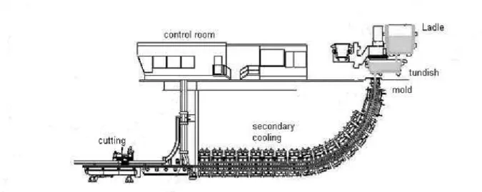
Figure 1: Continuous casting machine
FEM matrices is presented in [6]. We note that in our method it is sufficient to construct only 2D- and 1D-matrices. Therefore, it is obvious that the model is com-putationally much more efficient than in the case of using the ordinary 3D-brick elements.
4 Experimental Setup
Evaluation of cooling patterns and their assessment with respect to cost function (1) was done using the described mathematical model implemented in the form of a com-puter simulator. Its principal task is to dynamically track the temperature field in the slab as a function of process pa-rameters. In this study it was applied under the assumption of steady-state caster operation, and the search for optimal cooling patterns performed in the off-line manner. A single simulator run takes about 40 seconds on a 1.8 GHz Pentium IV computer.
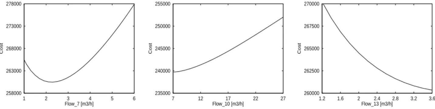
Before the integration of the simulator with the opti-mization algorithms, a number of simulator runs were per-formed to get an initial insight into the properties of the fit-ness landscape associated with the optimization problem. Specifically, the cost was analyzed as a function of individ-ual parameters and pairs of parameters, while keeping the remaining parameters fixed at the values from the middle of their intervals.
The resulting plots show simple dependencies between the parameters and cost function in the form of monotonic or at most U-shaped curves and surfaces (see examples in Figures 2 and 3). They are much simpler than usual ar-tificial test functions for numerical optimization, which is understandable because of the underlying physical process. Similar properties were found in the analysis of the fitness landscapes in parameter tuning for a continuous casting machine at the Acroni steel plant in Jesenice, Slovenia [11]. However, one should bear in mind that such analyses offer a very limited view of the problem characteristics. Never-theless, the real difficulty comes with high dimensionality
of the problem, as there are 18 independent process param-eters subject to optimization.
Before the application of optimization procedures one has to decide whether to search for optimal solutions in continuous or discretized parameter space. In analogy to previous studies performed on similar task from the Acroni steel plant [9, 14, 8], the discrete version was considered. The rationale behind it is in the engineering approach to coolant flow tuning where it is meaningless to consider changes below certain amount as they do not reflect in changing the cost value. For the purpose of numerical ex-periments three discretizations were defined, a very rough one for initial tests of the optimization algorithms, another one with medium step sizes to refine the results, and the one with the uniform step size of 0.1 m3/h which is the
mini-mum change considered in practice for all coolant flows (see Table 2).
Given these dicretizations, one can to calculate the num-ber of possible parameter settings. For a parameter from the interval [pmin
i , pmaxi ] with step size pstepi , there are vi =b(pmaxi −pmini )/pstepi c+ 1values possible, and the
total number of settings isv = QNp
i=1vi, whereNp is the
number of parameters. This results in4.6·1012 possible
setting for discretization 1, 4.9·1023for discretization 2,
and4.7·1033for discretization 3.
5 Numerical Experiments and
Results
7
11 15
19
23 7
11 15
19 23
230000 245000 260000
Flow_1 [m3/h]
Flow_10 [m3/h] 1
3 5
7 1 2
3 4
5 6 250000
275000 300000
Flow_4 [m3/h]
Flow_8 [m3/h] 2
4 6
8
10 2
3 4
5 260000
275000 290000
Flow_5 [m3/h]
Flow_14 [m3/h]
Figure 3: Examples of cost function dependencies on pairs of process parameters
Table 2: Parameter discretizations used in the optimiza-tion process; #val denotes the number of values possible for each parameter
Discretization 1 Discretization 2 Discretization 3
Flow Step Step Step
no. [m3/h] #val [m3/h] #val [m3/h] #val
1 4.7 5 1.0 20 0.1 191
2 8.6 5 1.0 35 0.1 348
3 6.6 5 1.0 27 0.1 267
4 1.6 5 0.5 13 0.1 65
5 1.8 5 0.5 15 0.1 74
6 1.4 5 0.2 29 0.1 58
7 1.3 5 0.2 27 0.1 53
8 1.2 5 0.2 25 0.1 49
9 1.2 5 0.2 26 0.1 51
10 4.7 5 1.0 20 0.1 191
11 8.6 5 1.0 35 0.1 348
12 6.6 5 1.0 27 0.1 267
13 0.5 5 0.2 12 0.1 24
14 0.5 5 0.2 11 0.1 21
15 0.1 6 0.1 6 0.1 6
16 1.3 5 0.2 27 0.1 53
17 1.2 5 0.2 25 0.1 49
18 1.2 5 0.2 26 0.1 51
population of 20 solutions, applying arithmetic crossover and Gaussian mutation adjusted to perform vector varia-tion with prescribed discretizavaria-tion. The local optimizavaria-tion algorithm relied on the neigborhod relationship among can-didate solutions. Two solutions were considered neighbors if differing in thei-th vector component for±pstepi . In this way each solution, with the exception of those on the edge of the search space, had 2Np = 36neighbors. The
al-gorithm started from a randomly selected point and was
restarted after reaching a local minimum.
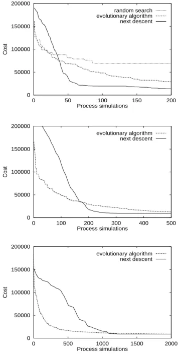
For each of the three search space discretizations the al-gorithms were run five times and their results evaluated statistically. The number of solutions checked (parame-ter settings evaluated) in each algorithm run was 200 for discretization 1, 500 for discretization 2, and 2000 for dis-cretization 3. No other parameter adjusting was involved as this empirical study was a preliminary one.
The performance of the algorithms under different search space discretizations is illustrated in Figure 4 and the results in terms of cost summarized in Table 3. For discretization 1, the performance of random search is also shown to provide an empirical upper bound for the results. In this case, the local optimization algorithm clearly out-performs the evolutionary algorithm, but the cost values produced are still high which indicates the discretization is too rough to allow for detection of the near-optimal solu-tion. With the refinement of discretization better results are found by both methods and their performance com-pares differently. The finer the discretization, the closer the final results, while in the initial stage of the search the evolutionary algorithm outperforms the local optimization algorithm. The solutions found with local optimization are however not dispersed as with the evolutionary algo-rithm. It turns out that the more complex the search space the more obvious the efficiency of the evolutionary algo-rithm in identifying the promising regions which suggests an appropriate hybrid of the two algorithms would reduce the number process simulations needed in the optimization procedure.
0 50000 100000 150000 200000
0 50 100 150 200
Cost
Process simulations random search evolutionary algorithm next descent
0 50000 100000 150000 200000
0 100 200 300 400 500
Cost
Process simulations evolutionary algorithm
next descent
0 50000 100000 150000 200000
0 500 1000 1500 2000
Cost
Process simulations evolutionary algorithm
next descent
Figure 4: Performance of the optimization algorithms av-eraged over five runs of each algorithm for parameter dis-cretizations 1 (top), 2 (center), and 3 (bottom)
Table 3: Summary of the optimized cost values found for three parameter discretizations; EA denotes the steady-state evolutionary algorithm, and ND next descent local optimization
Discr. Method Best Average Worst St. dev.
1 EA 24988.8 28965.9 32842.5 2800.8
ND 13417.9 13794.9 15062.7 716.3
2 EA 10371.3 12466.6 14092.0 1790.4
ND 9592.9 9592.9 9592.9 0.0
3 EA 9078.5 9194.0 9247.2 73.7
ND 9070.4 9070.4 9070.4 0.0
be compared with the empirical settings used in practice, and checked for possible contribution to the improvement of steel quality.
6 Conclusion
Optimization of coolant flow settings in continuous casting of steel is a key to higher product quality. It is nowadays to a high degree performed through virtual experimenta-tion involving numerical process simulators and advanced optimization techniques. In this preliminary study of op-timizing 18 cooling water flows for a Rautaruukki casting machine under steady-state conditions, an empirical inves-tigation of the problem properties was done, two stochastic algorithm applied and their performance compared.
The results indicate the importance of the applied search space discretization and suggest the construction of a hy-brid algorithm to find near-optimal solutions in smaller number of solution evaluations. With the same objective in mind, the algorithms will be systematically tuned and en-hanced with the mechanisms of gradual refinement of the search focus, such as dynamic parameter encoding [15] or the multilevel technique [12]. On the practical side, the op-timized coolant flows will be evaluated with respect to the settings used on the caster machine and checked for poten-tial further improvements of the casting process.
Acknowledgement
This work was supported by the Slovenian Research Agency and the Academy of Finland under the Slovenian-Finnish project BI-FI/04-05-009 Numerical Optimization of Continuous Casting of Steel, by the European Sci-ence Foundation under COST 526: Automatic Process Optimization in Materials Technology(APOMAT), and by the Slovenian Research Agency under the Research Pro-gramme P2-0209-0106 Artificial Intelligence and Intelli-gent Systems.
References
[1] T. Bäck, D. B. Fogel, Z. Michalewicz (Eds.). Hand-book of Evolutionary Computing, Institute of Physics Publishing, Bristol, Philadelphia, and Oxford Univer-sity Press, New York, Oxford, 1997.
[2] N. Chakraborti, R. Kumar, D. Jain. A study of the continuous casting mold using a Pareto-converging genetic algorithm.Applied Mathematical Modelling, 25 (4): 287–297, 2001.
[7] C. M. Elliot, J. R. Ockendon. Weak and Variational Methods for Moving Boundary Problems. Pitman Publishing, Boston, 1982.
[8] B. Filipiˇc. Efficient simulation-based optimization of process parameters in continuous casting of steel. In: D. Büche, N. Hofmann (Eds.),COST 526: Auto-matic Process Optimization in Materials Technology: First Invited Conference, pp. 193–198, Morschach, Switzerland, 2005.
[9] B. Filipiˇc, T. Robiˇc. A comparative study of coolant flow optimization on a steel casting machine. Pro-ceedings of the 2004 Congress on Evolutionary Com-putation, Portland, OR, USA, Vol. 1, pp. 569-573. IEEE, Piscataway, 2004.
[10] B. Filipiˇc, B. Šarler. Evolving parameter settings for continuous casting of steel. Proceedings of the 6th European Conference on Intelligent Techniques and Soft Computing EUFIT’98, Vol. 1, pp. 444–449. Ver-lag Mainz, Aachen, Germany, 1998.
[11] B. Filipiˇc, B. Šarler. An empirical investigation into the Properties of Coolant Flow optimization in the Steel Production Process. In: B. Zajc, A. Trost (Eds.),
Proceedings of the Fourteenth International Elec-trotechnical and Computer Science Conference ERK 2005, Portorož, Slovenia, Vol. B, 59–62. Slovenia Section IEEE, Ljubljana, 2005.
[12] P. Korošec, J. Šilc. The multilevel ant stigmergy algo-rithm: an industrial case study.Proceedings of the 8th Joint Confeence on Information Sciences JCIS 2005, pp. 475–478, Salt Lake City, Utah, USA.