ISSN 2307-7743 http://scienceasia.asia
A SURFACE FAMILY WITH A COMMON ASYMPTOTIC CURVE IN THE EUCLIDEAN 3-SPACE
RASHAD A. ABDEL-BAKY1,2
Abstract. In this paper, we offer an approach for study the problem on how to construct
a surface family from a given asymptotic curve and we deduce the necessary and sufficient condition for the given curve to be the asymptotic curve for the parametric surface. Mean-while, some representative curves are chosen to construct the corresponding surfaces which possess these curves as asymptotic curves. The extension to ruled and developable surfaces is also outlined. Finally, we demonstrated some interesting ruled and developable surfaces about the subject.
1. Introduction
In the 3-dimensional Euclidean space, asymptotic curve on a surface is an intrinsic geo-metric feature that plays an important role in a diversity of applications. It is a useful tool in surface analysis for exhibiting variations of the principal direction and has been a long-standing research focus in Differential Geometry [1, 2]. Many studies on dealing with asymptotic curves have been reported. Hartman and Wintner [3] showed that the degree of smoothness is an important notion in the classical theory of asymptotic curves of non-positive Gaussian curvature, which is usually left unspecified. Kitagawa [4] proved that ifM
is a flat torus isometrically immersed in a unit 3-sphere, then all asymptotic curves onM are periodic. Garcia and Sotomayor [5] studied the simplest qualitative properties of asymptotic curves of a surface immersed in the Euclidean 3-space E3. Garcia et al. [6] studied im-mersions of surfaces into E3 whose nets of asymptotic curves are topologically undisturbed under small perturbations of the immersion, which can then be described as structurally asymptotic stable. Contopoulos [7], proved that in order to find a set of escaping orbits of stars in a stellar system, it is necessary to find asymptotic curves of the Lyapunov orbits, because any small outward deviation from an asymptotic orbit will lead a star to escape from the system. The work of Contopoulos considered the asymptotic orbits of mainly unstable orbits, with a particular emphasis on the Lyapunov orbits, and found sets of escaping orbits with initial conditions on asymptotic curves. Efthymiopoulos et al. [8] concluded that the diffusion of any chaotic orbit inside the contours follows essentially the same path defined
Key words and phrases. Serret–Frenet formulae; asymptotic curve; ruled surface; marching-scale functions.
c
by the unstable asymptotic curves that emanate from unstable periodic orbits inside the contours.
In practical applications, the concept of family of surfaces having a given characteristic curve was first introduced by Wang et.al. [9] in Euclidean 3-space. The basic idea is to regard the wanted surface as an extension from the given characteristic curve , and represent it as a linear combination of the marching-scale functionsu(s, t),v(s, t),w(s, t) and the three vector functionst(s),n(s),b(s), which are the unit tangent, the principal normal and the binormal vector of the curve respectively. With the given characteristic curve and isoparametric constraints, they derived the necessary and sufficient conditions for the correct parametric representation of the surface pencil. This principal has been used treated extensively in the works (see for example [10-16]).
However, the relevant work on surfaces through asymptotic curve is rare. It is an important and interesting problem in practical applications. Therefore, research on designing a surface from a given curve is attractive. Inspired by Wang et al. [10], in this paper, we offer an alternative approach for designing surfaces from a given asymptotic curve. We not only construct a surface possessing a given curve as an asymptotic curve, but also give a concrete expression of the surface. Moreover, the extension to the ruled and developable surfaces is also outlined. Also, some representative curves are chosen to construct the corresponding surfaces which possessing these curves as asymptotic curves.
2. Preliminaries
In this section we list some notions, formulas and conclusions for space curves, and ruled surfaces in Euclidean 3-space E3which can be found in the textbooks on differential geometry
(See for instance Refs. [1-3]).
A curve is regular if it admits a tangent line at each point of the curve. In the following discussions, all curves are assumed to be regular. Given a spatial curveα: s →α(s), which is parameterized by arc length parameter s. We assume α..(s) 6= 0 for all s ∈ [0, L], since this would give us a straight line. In this paper, α.(s) and α0(r) denote the derivatives of α with respect to arc-length parameter s and arbitrary parameter r, respectively. For each point of α(s), the set {t(s),n(s),b(s)}is called the Serret–Frenet Frame alongα(s), where t(s) = α.(s), n(s) = α..(s)/
..
α(s) and b(s) = t(s)×n(s) are the unit tangent, principal normal, and binormal vectors of the curve at the point α(s), respectively. The arc-length derivative of the Serret–Frenet frame is governed by the relations:
(1)
.
t(s)
.
n(s)
.
b(s)
=
0 κ(s) 0
−κ(s) 0 τ(s) 0 −τ(s) 0
t(s) n(s) b(s)
where the curvatureκ(s) and torsionτ(s) of the curve α(s) are defined by
(2) κ(s) =
..
α(s), τ(s) =
det(α.(s),α..(s),α...(s))
..
α(s)
2 .
In the majority of practical cases, the parameter of the curve is usually not in arc-length representation. Given the parametric curve
α(r) = (α1(r), α2(r), α3(r)),0≤r ≤H,
where the parameter ris not the arc length. The components of the Serret–Frenet frame are defined by [1-3]:
(3) t(r) = α
0 (r)
kα0(r)k, b(r) =
α0(r)×α 00
(r)
α
0
(r)×α00(rr)
, n(r) = b(r)×t(r),
and the corresponding Serret-Frenet frame is given by
(4)
t0(r) n0(r) b0(r)
=
0 κ(r)α
0
(r) 0 −κ(r)α
0
(r) 0 τ(r)
α
0 (r)
0 −τ(r)α
0
(r) 0
t(r) n(r) b(r)
.
3. A surface family with an asymptotic curve
Consider the construction of a surface from a unit speed space curveα=α(s), 0≤s≤L, such that the surface tangent plane is coincident with the curve osculating plane. Expressing the surface in terms of Serret–Frenet frame{t(s), n(s), b(s)} along α(s) as:
(5) M :P(s, t) =α(s) +u(s, t)t(s)+v(s, t)n(s); 0≤t≤T, 0≤s≤L,
where u(s, t), and v(s, t) are all C1 functions. If the parameter t is seen as the time, the
functions u(s, t), and v(s, t) can then be viewed as directed marching distances of a point unit in the timet in the directiont, andn, respectively, and the position vectorα(s) is seen as the initial location of this point.
It is easily checked that the two tangent vectors ofM are given by:
(6) Ps= (1 +us−vκ)t+ (vs+uκ)n+vτb, Pt=utt+vtn.
)
The lowercase subscript letters s, and t denote partial derivatives corresponding to the indicated variable, e.g., Ps = ∂∂sP, Pt = ∂∂tP. Consequently, the normal vector of the surface
is given by:
(7) N(s, t) := Ps×Pt=η1(s, t)t(s) +η2(s, t)n(s) +η3(s, t)b(s),
where
(8) η1(s, t) =−v(s, t)τ(s)vt(s, t), η2(s, t) = v(s, t)τ(s)ut(s, t),
η3(s, t) = (1 +us(s, t)−v(s, t)κ(s))vt(s, t)−(vs(s, t) +u(s, t)κ(s))ut(s, t).
Since the curve α(s) is an isoparametric on the surface, there exists a parameter t = t0 ∈
[0, T] such that P(s, t0) =α(s); that is,
(9) u(s, t0) = v(s, t0) = 0, 0≤t0 ≤T, 0≤s≤L,
and thus when t=t0—i.e., along the curve α(s)—the surface normal is
(10) N(s, t0) =η3(s, t0)b(s),
where
(11)
η1(s, t0) = 0,
η2(s, t0) = 0,
η3(s, t0) =vt(s, t0)6= 0.
Combining conditions (3.5) and (3.7), we have found the necessary and sufficient conditions for the surface P(s, t) to have the curve α(s) as an isoasymptotic.
Hence, we can state the following theorem:
Theorem 3.1. The given spatial curveα(s) is an isoasymptotic curve on the surfaceP(s, t) if and only if
(12) u(s, t0) =v(s, t0) = 0,
vt(s, t0)6= 0, 0≤t0 ≤T, 0≤s≤L.
)
Obviously, Eqs. (3.8) is more elegant and convenient for applications than those in [14]. The important point to note here is the technique we have used. In Ref. [9], for simplification and better analysis, the marching-scale functionsu(s, t),and v(s, t) can be decomposed into two factors:
(13) u(s, t) = l(s)U(t),
v(s, t) =m(s)V(t).
Here l(s), m(s), V(t) and W(t) are C1 functions and l(s),and m(s) are not identically zero. Thus, from Theorem 3.1, we can get the following corollary.
Corollary 3.1. The necessary and sufficient condition of the curve α(s) being an isoasymp-totic curve on the surface P(s, t) is
(14) U(t0) =V(t0) = 0, 0≤t0 ≤T, 0≤s ≤L,
m(s)dV(t0)
dt 6= 0⇔m(s)6= 0, and dV(t0)
dt =const6= 0.
)
For the case when the marching-scale functions depend only on the parameter t; that is,
l(s) =m(s) = 1. By simplifying, condition (3.10) can be represented as
(15) UdV((tt0) =V(t0) = 0, 0)
dt 6= 0, 0≤t0 ≤T.
)
The corresponding isoparametric asymptotic surface family becomes
3.1. Simple surfaces with a common asymptotic curve. Now, we are going to deal with and construct some representative examples to verify the method. They also serve to verify the correctness of the formulae derived above.
Example 1. Ifp0 = (0,0,0),p1 = (0,1,1),andp2 = (1,2,0) are the points in the Euclidean
3-space E3, then the quadratic B´ezier curve can be expressed as
α(r) = r(1−r)2p0+ 2r(1−r)p1+r2p2, 0≤r≤1.
It is easy to show that
κ(r) =
√ 6
2(5r2−4r+ 2)32, τ(r) = 0.
After simple computation, we get:
t(r) = r,1,f−(2rr)+1,
n(r) =2(1−r)√,2−5r,−(2+r)
6f(r)
,
b(r) =
−√2 6,
1
√
6,− 1 √ 6 ,
where f(r) = √5r2−4r+ 2. Choosing U(t) = βt, and V(t) = γt, γ 6= 0, and t ∈ [0, T].
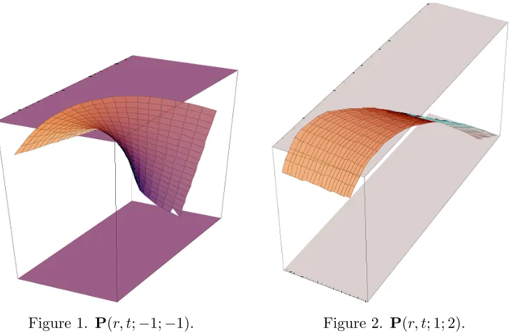
Obviously, Eq. (3.11) is satisfied. Thus, we obtain the following isoparametric asymptotic surface family:
P(r, t;β;γ) = (r2,2r,2r−2r2) +t(β, γ,0)
r l(r)
1
l(r)
−2r+1
l(r) 2(1√−r)
6l(r)
2−5r
√
6l(r)
−√(2+r) 6l(r)
−√2 6 1 √ 6 − 1 √ 6 ,
where 0 ≤ t ≤ 1, and 0 ≤ r ≤ 1. The parameters β and γ can control the shape of the surface. For β=−1, and γ =−1, the surface is shown in Fig. 1. Figure 2 shows the surface with β = 1, and γ = 2.
Example 2. In this example, we construct surface family in which all the surfaces share an asymptotic circular helix represented as
α(r) = (acosr, asinr, br), a >0, b6= 0, 0≤r≤2π.
It is easy to show that:
t(r) = √ 1
a2+b2(−asinr, acosr, b),
n(r) = (−cosr,−sinr,0),
b(r) = √ 1
a2+b2(bsinr,−bcosr, a).
A- ChoosingU(t) = βt, andV(t) = γt, γ 6= 0, andt∈[0, T], we obtain the following surface family:
P(r, t;β;γ) = (acosr, asinr, br) +t(β, γ,0)
−a
√
a2+b2 sinr
a
√
a2+b2 cosr
b
√
a2+b2
−cosr −sinr 0
b
√
a2+b2 sinr −b
√
a2+b2 cosr
a
√
a2+b2
Figure 1. P(r, t;−1;−1). Figure 2. P(r, t; 1; 2).
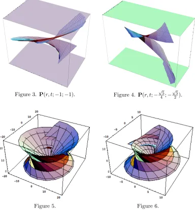
Here, we chose t ∈[0,4], and a = 2, b= 1. For β =−1, and γ = −1, the surface is shown in Fig. 3. Figure 4 shows the surface with β=−
√
5
4 , andγ =−
√
5 2 .
B- By choosing marching-scale functions as
u(s, t) = (1 + sin(t)) +
4
X
k=2
a1k(1 + sin(t))k,
v(s, t) = cos(t) +
4
X
k=2
a2kcosk(t), t0 = 0, t0 = 3π/2, a1k, a2k ∈R,
then Eqs. (3.11) are satisfied. Ifa =b = 1,a1k= 5, anda2k = 0.5, then we obtain a member
in the family as shown in in Figure 5. Figure 6 shows the surface with a= b = 1, a1k = 3,
and a2k= 0.5.
Note that we could continue this series of surfaces, by choosing yet another combination of characteristic curve, or number of curves to interpolate.
4. Ruled surfaces with a common asymptotic curve
In the following, we will construct a ruled surface from a given asymptotic curve. For the ease of discussion, let us assume that α =α(s) is a unit speed curve in the Euclidean 3-space E3, wheres is the arc length parameter. Suppose P(s, t) is a ruled surface with the
directrix α(s) and α(s) is also an isoparametric curve of P(s, t), then there exists t0 such
that P(s, t0) = α(s). This follows that the surface can be expressed as
Figure 3. P(r, t;−1;−1). Figure 4. P(r, t;− √
5 4 ;−
√
5 2 ).
Figure 5. Figure 6.
where d(s) denotes the direction of the rulings. According to the Eq. (3.12), we have
(17) (t−t0)d(s) =α(s) +u(s, t)t(s)+v(s, t)n(s), 0≤s≤L, with t, t0 ∈[0, T],
which is a system of two equations with two unknown functions u(s, t), and v(s, t). The solutions of the above system can be deduced as
(18) u(s, t) = (t−t0)<d(s),t(s)>= det(d(s),n(s),b(s))
v(s, t) = (t−t0)<d(s),n(s)>= det(d(s),b(s),t(s)).
Next, we need to check if the curveα(s) is also asymptotic on the surfaceP(s, t) by using the conditions given in Theorem 3.1. It is evident that in this case, these conditions become
(19) det(d(s),n(s),b(s)) = 0, det(d(s),b(s),t(s))6= 0.
It follows that at any point on the curveα(s), the ruling directiond(s) must be in the plane spanned byt(s), and n(s). On the other hand, the ruling directiond(s), and the vectort(s) must not be parallel. This implies
(20) d(s) = β(s)t(s) +γ(s)n(s), γ 6= 0, 0≤s≤L,
for some real functions β(s), and γ(s). Substituting it into the expressions in Eq. (4.3), we get
(21) β(s)t=u(s, t), γ(s)t=v(s, t), γ 6= 0, 0≤s≤L.
Hence, the isoparametric asymptotic ruled surface family with the common asymptotic di-rectrix α(s) can be expressed as
(22) M :P(s, t;β;γ) =α(s) +t(β(s)t(s) +γ(s)n(s)), γ 6= 0, 0≤s ≤L, 0≤t≤T,
where the functions β(s), and γ(s) can control the shape of the surface pencil. Moreover, the normal vector to the ruled surface P(s, t;β;γ) is
(23) N(s, t) = −tγτ(γt+βn) + [γ(1 +t(
.
β−γκ)−tβ(γ. +βκ)b,
and thus when t= 0— i.e., along the curve α(s)— the surface normal is
(24) N(s,0) =−γb.
Coincidence of the osculating plane of α(s) with the tangent plane of P(s, t;β;γ) identifies the curve as an asymptotic curve of the surface.
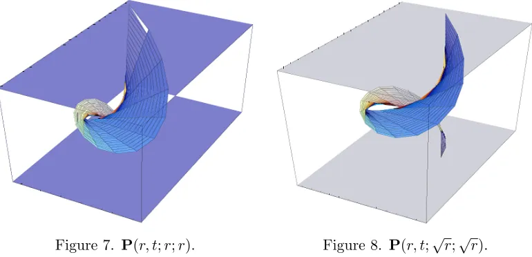
It should be pointed out that in this model, there exist two asymptotic curves passing through every point on the curve α(s): one is α(s) itself and the other is a straight line in the direction d(s) as given in Eq. (4.4). Every member of the isoasymptotic ruled surface pencil is decided by two pencil parametersβ(s), andγ(s), i.e., by the direction vector function d(s). In Example 2: Forβ(r) =γ(r) = r, witht∈[0,2], anda= 2, b= 1 the corresponding ruled surface is shown in Fig. 7. Figure 8 shows the surface withβ(r) =γ(r) = √r.
4.1. Developable surfaces. A special class of ruled surfaces, the developable surfaces, is characterized by a constant surface normal along each ruling. A surface is developable if and only if it is the envelope of a one–parameter family of planes. Developable surface and asymptotic curve play an important role in geometric design and surface analysis, see for example [11-16].
Figure 7. P(r, t;r;r). Figure 8. P(r, t;√r;√r).
relationship between the given curve α(s) and its isoparametric developable surface. In the light of above statements, we have:
(25) <d×d.,α. >= 0.
From Eq. (4.9), we note that there are two possible cases, as presented in the following: The first case is when
(26) d×d. =0⇔β. −γκ=µβ, γ. +βκ=µγ, τ γ = 0,
where µ=µ(s) is a differentiable function. In this case, the ruled surface is referred to as a cylindrical surface. We may rewrite Eq. (4.10) as follows:
. β−γκ
β =
. γ+βκ
γ =µ, τ γ = 0.
Forγ 6= 0, it follows thatτ = 0, and we have:
(27) β(s) =γtan(
s
Z
0
γ2κds).
Therefore, the cylindrical surface M is uniquely defined by the asymptotic curve α=α(s) and the differentiable function γ(s).
Corollary 4.1. Planar curves are isoasymptotic to cylindrical surfaces. By similar argument, we can also have the following:
d×d. 6=0.
This implies thatM is a non-cylindrical surface. Therefore, the first derivative of the directrix is
(28) α.(s) =
.
C(s) +µ(s)
.
where
.
C is the first derivative of the striction curve, µ(s) is a smooth function [1, 2]. Sub-stituting Eq. (4.12) into Eq. (4.9) gives
(29) <d×d.,
.
C>= 0.
Similarly, there are two possible cases which satisfy Eq. (4.13), as presented in the follow-ing: The first case is when the first derivative of the striction curve is
.
C= 0. Geometrically this condition implies that the striction curve degenerates to a point, and the ruled surface becomes a cone; the striction point of a cone is commonly referred to as the vertex. There-fore, the surface represented by Eq. (4.6) is a cone if and only if there exists a fixed pointC and a function µ(s) such that
1 +µκγ = d
ds(µβ), 0 = µκβ+ d
ds(µγ), γµτ = 0.
Forγ = 0, it follows thatτ = 0 (αis planar curve), which implies the following conditions:
1 +µκγ = d
ds(µβ), 0 = µκβ+ d ds(µγ).
Let β = 0, where µ(s) is a non-constant function. In this case, according to α is planar curve, we have
1 +µκγ= 0, 0 = d
ds(µγ),
it follows that α is a planar curve with constant curvature, i.e.,
µγ=−1
κ =const.,
Corollary 4.2. In Euclidean 3-space, there is no a cone whose base curve is a planar asymptotic curve.
The second case is whenC. 6= 0. Since det(C.,d,d.) = 0, <C.,d.>=0, and <d,d. >= 0, we can get
.
Ckd. This means the surface is a tangent surface parameterized by
P(s, t) =α(s) +tα.(s)
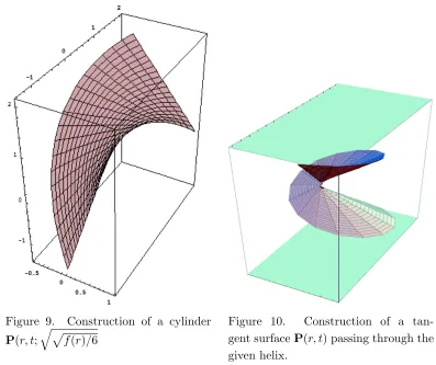
whereα(s) is called the curve of regression. Generally, when the given curve does not satisfy Corollaries 4.1 and 4.3, it is isoasymptotic to a tangent surface (Fig. 9).
5. Conclusion
Figure 9. Construction of a cylinder
P(r, t; q
p
f(r)/6
Figure 10. Construction of a tan-gent surfaceP(r, t) passing through the given helix.
given asymptotic curve, which is quite in accord with the practice in industry design and manufacture.
References
[1] G. Farin. Curves and Surfaces for Computer Aided Geometric Design, 2nd ed. New York: Academic Press, 1990.
[2] M.P. Do Carmo. Differential Geometry of Curves and Surfaces. Englewood Cliffs: Prentice Hall, 1976. [3] P. Hartman, A. Wintner. On the asymptotic curves of a surface. Amer. J. Math. 1951; 73(1): 149–72. [4] Y. Kitagawa. Periodicity of the asymptotic curves on flat tori in S3. J. Math. Soc. Japan 1988; 40(3):
457–96.
[5] R. Garcia, J. Sotomayor. Structural stability of parabolic points and periodic asymptotic lines. Mat. Contemp. 1997; 12: 83–102. Workshop on real and complex singularities (Sao Carlos, 1996).
[6] R. Garcia, C. Gutierrez, J. Sotomayor. Structural stability of asymptotic lines on surfaces immersed in R3. Bull. Sci. Math. 1999; 123(8): 599–622.
[7] G. Contopoulos. Asymptotic curves and escapes in Hamiltonian systems. Astron. Astrophys. 1990; 231: 41–55.
[8] C. Efthymiopoulos, G. Contopoulos, N. Voglis. Cantori, islands and asymptotic curves in the stickiness region. Celestial Mech. Dynam. Astronom. 1999; 73: 221–30.
[10] E. Kasap, F. T. Akyildiz, K. Orbay. A generalization of surfaces family with common spatial geodesic, Appl. Math. Comput., 201 (2008), 781-789.
[11] E. Kasap and F.T. Akyildiz. Surfaces with common geodesic in Minkowski 3-space, Appl. Math. Com-put., 177 (2006), 260-270.
[12] G. Saffak, E. Kasap. Family of surface with a common null geodesic, Internat. J. Phys. Sci., Vol. 4(8) (2009), 428-433.
[13] C.Y. Li, R. H. Wang, C. G. Zhu. Parametric representation of a surface pencil with a common line of curvature, Comput. Aided Des., 43 (9) (2011), 1110-1117.
[14] E. Bayram, F. Guler, E. Kasap. Parametric representation of a surface pencil with a common asymptotic curve, Comput. Aided Des., 44 (2012), 637-643.
[15] C.Y. Li, R. H. Wang, C. G. Zhu. An approach for designing a developable surface through a given line of curvature, Computer-Aided Design, 2013, 45: 621–627.
[16] C.Y. Li, R. H. Wang, C. G. Zhu. A generalization of surface family with common line of curvature, Applied Mathematics and Computation , 2013, 219: 9500–9507.
1
Present address: Department of Mathematics, Sciences Faculty for Girls, King Abdu-laziz University, P.O. Box 126300, Jeddah 21352, SAUDI ARABIA
2