AN APPLICATION OF MOTION CORRECTION METHODS
TO THE ALIGNMENT PROBLEM IN NAVIGATION
1Boris I. Ananyev
Krasovskii Institute of Mathematics and Mechanics,
Ural Branch of Russian Academy of Sciences, Ekaterinburg, Russia, [email protected]
Abstract: In this paper, we apply some motion correction methods to the alignment problem in navigation. This problem consists in matching two coordinate systems having the common origins. As a rule, one of the systems named as basic coordinate system is located at a ship or airplane. The dependent coordinate system belongs to another object (e.g. missile ) that starts from the ship. The problem is considered with incomplete information on state coordinates which can be measured with disturbances without statistical description.
Key words: Alignment problem, Motion correction, Incomplete information, Set-membership description of uncertainty.
Introduction
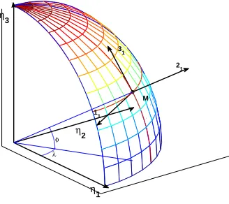
Alignment is the process whereby the orientation of the axes of an inertial navigation system is determined with respect to the reference axis system. The basic concept of aligning an inertial navigation system is quite simple and straightforward. However, there are many complications that make alignment both time consuming and complex. Consider a simulated transport ship-airplane system. Suppose that the base coordinate system (BCS) of the ship is correct. Let −→Ω1 be the
absolute angular velocity of the BCS in the motionless coordinate systemη1, η2, η3. The projection
Ω2
1 on vertical 21 equals zero. This system is shown on Fig. 1. The axis 11 is directed along the
21
M 31
11
η1 η2
φ λ
η3
Figure 1. The section of Earth sphere and the base coordinate system.
parallel to the west. The axis 21 is the local vertical. The axis 31 is directed along the meridian
to the north. The position of the dependent coordinate system (DCS) related to the airplane or
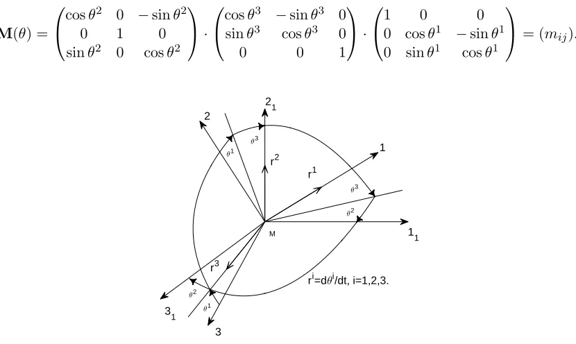
the missile with respect to the BCS is estimated by the Krylov angles. In Fig. 2, one can see the sequence of clockwise rotations: θ1 around axis 1,θ3 around new axis 3, andθ2 around new axis 2 coinciding now with 21.
Thus, the transition of coordinates of a vector f~in the DCS to new coordinates in the BCS is occurred by the formulaf~1=M(θ)f~, where the matrix of direction cosines is of the form
M(θ) =
cosθ2 0 −sinθ2
0 1 0
sinθ2 0 cosθ2 ·
cosθ3 −sinθ3 0 sinθ3 cosθ3 0
0 0 1
·
1 0 0
0 cosθ1 −sinθ1
0 sinθ1 cosθ1
= (mij).
1 1
31
2 1 2
1
3
r1 r2
r3
θ3
θ3
θ1 θ1
θ2
θ2
ri=dθi/dt, i=1,2,3. M
Figure 2. The sequence of clockwise rotations.
Projecting the equality ω~ =~θ˙1+θ~˙3+~θ˙2 for the angular velocities on the axes of the DCS, we obtain the kinematic Krylov equations
˙
θ1 =ω1−θ˙2sinθ3, θ˙2= (ω2cosθ1−ω3sinθ1)/cosθ3, θ˙3 =ω2sinθ1+ω3cosθ1, (0.1) whereωi are the projections of the relative angular velocity. These projections are related with the absolute velocities by the formulas
ωi = Ωi−m1iΩ11−m3iΩ31+εi, i∈1 : 3, (0.2)
whereεi are the projections of an uncertain drift.
For measurements, the differences of accelerometer readings in the DCS and BCS are used. These accelerometers are on the axes and gage the nongravity acceleration ~a = −→wM −~g. Let
ai be accelerometers readings in the DCS and ai1 be gage readings in the BCS. Therefore, the measurement equations are of the form
y1 = (m11−1)a11+m21a21+m31a31+w1, y2=m12a11+ (m22−1)a21+m32a31+w2, y3=m13a11+m23a12+ (m33−1)a31+w3,
(0.3)
where wi are uncertain leavings of zero. About drifts εi in (0.2), the assumption is accepted that they are constant but unknown. Uncertain functions in relations (0.3) satisfy the integral inequalities
Z T
0
Let~i1,~i2,~i3 be the unit direction vectors of the BCS. The velocity of point M equals
4~vM =−→Ω1×−→R =
~i1 ~i2 ~i3
Ω11 0 Ω31
0 R 0
,
where R is the radius of Earth. From here we find the projections of velocity on the BCS axes:
v11 = −RΩ31, v12 = 0, v13 = RΩ11. Computing the derivative of ~vM, we get the acceleration
−
→wM = f−→wM +−→Ω1×~vM in the form of the sum of relative and translation accelerations. So, the
accelerometers readings in BCS are of the form:
a11 =−R ˙Ω31, a21 =g−v2/R, a31 =R ˙Ω11, (0.5) where v is the velocity magnitude. As R = 6370 km and the velocity of the ship on water is no more than 20 m/c, we assume a21 =g.
Further we consider some approaches from motion correction for solving the alignment problem. This problem in inertial navigation was first in detail considered in [1]. Russian books devoted to this topic are [2–5]. The alignment problem was mostly solved in [1–5] by statistical methods with the help of Kalman filter or its modifications. On the other hand, in [2, 6] it was noted that the statistics of disturbances often happens incomplete or completely absent. Therefore, it is natural to use here the minimax methods from books [7, 8]. Thus, all the disturbances in our paper are deterministic.
Consider only the case of small angular deviations (no more than several degrees). Equations (0.1) are replaced by the follwing ones:
˙
θ1 =u1+ε1−θ2Ω31−θ3u2, θ˙2=u2+ε2+θ3Ω11−θ1Ω31−θ1u3,
˙
θ3 =u3+ε3+θ2Ω11+θ1u2.
(0.6)
Here,ui = Ωi−Ωi1,i∈1 : 3. In the linear approximation, the differences of accelerometer readings in (0.3) are equal to
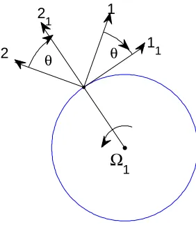
y1 =gθ3+a31θ2+w1, y2 =−a11θ3+a31θ1+w2, y3=−a11θ2−gθ1+w3. (0.7) Equations (0.6) contain the multiplications of controls and state variables, but, in the case of small angles and angular velocities these terms may be neglected. In the specific case of movement on the equator under condition θ1 = θ2 ≡ 0, we assume θ = θ3 as shown on Fig. 3. The angular velocity Ω1 = Ω31 6= 0 under given movement and the rest projections of absolute angular velocity
are equal to zero. We have
˙
θ=u+ε, ε˙= 0, y=gθ+w, (0.8)
where the first equation from (0.7) is taken as the output.
1. Set-membership background
So, we consider a determinate n-dimensional linear system of the form
˙
x(t) =A(t)x+B(t)u+C(t)v, t∈[0, T], (1.1) assuming that the initial statex0of system (1.1) is completely unknown, the matricesA(t), B(t), C(t),
Ω
1θ θ
2
1 2
1
1
1
Figure 3. System deviation in the simple model.
the system is added here. It corresponds to the case when drifts are not constants. The unknown functionv(·) and the disturbance w(·) in them-dimensional equation of measurement
y(t) =G(t)x(t) +w(t) (1.2)
are bounded by the constraint
Z T
0
|v(t)|2Q(t)+|w(t)|2R(t)dt≤1, (1.3)
where the symbol|x|2P equals x′P x, prime ′ means the transposition,Q(t), R(t) are symmetrical, positive-defined, and continuous matrices having suitable dimension. Constraint (1.3) involves that the elements of vector functionsv(·) andw(·) belong to the space L2[0, T]. We need the following
Assumption 1. The system (1.1),(1.2)underu≡0, v≡0, w≡0is completely observable [7]
on any subinterval [s, τ]⊂[0, T].
Assumption 1 means that the vector x(s) can be uniquely restored from the signal observed on [s, τ] if the disturbances are absent. Moreover, Assumption 1 holds if and only if
Z τ
s
X′(t, s)G′(t)G(t)X(t, s)dt >0,
whereX(t, s) is the fundamental matrix of system (1.1). We use piecewise-constant functionsu(t), for which
u(t)∈P ⊂Rp, (1.4)
whereP is a compact convex set. Constraint (1.4) is more realistic than integral constraints in [9]. The aim of the control is to minimize the terminal function |Dx(T)|, where | · | is the Euclidean norm andD ∈Rd×n is a matrix. The choice of uncertain parameters {x0, v(·), w(·)} may impede
1.1. Informational and compatible sets
At first, let us consider a set-membership estimation scheme for system (1.1), (1.2) under constraint (1.3).
Definition 1. A set X(t, y, u)⊂Rn is said to be the informational if it consists of all vectors x = x(t), which may realize in system (1.1), (1.2) with given signal y(τ), 0 ≤ τ ≤ t, the control u(τ), and some disturbances satisfying constraint (1.3).
To describe the informational set, we introduce the Bellman function
V(t, x) = inf
v(·) Z t
0
|v(s)|2Q(s)+|y(s)−G(s)x(s)|2R(s)ds
, x(t) =x.
The Bellman equation for V(t, x) is of the form:
Vt= min v
n
−(A(t)x+B(t)u(t) +C(t)v)′Vx+|v|2Q(t)+|y(t)−G(t)x|2R(t) o
, V(0, x) = 0. (1.5)
If the solution of equation (1.5) in any sense is found, the informational setX(t, y, u) is written as the inequality X(t, y, u) ={x:V(t, x)≤1}. Let us seek a solution of equation (1.5) in the form
V(t, x) =|x|2P(t)−2x′d(t) +g(t), (1.6) whereP(t) is a positive definite and continuously differentiable matrix, d(t) and g(t) are a contin-uously differentiable vector function and a function respectively. Substituting (1.6) into (1.5), we get
|x|2P˙(t)−2x′d˙(t) + ˙g(t) =|y(t)−G(t)x|2R(t)− |P(t)x−d(t)|2C(t)Q−1(t)C′(t)−
−2(A(t)x+B(t)u(t))′(P(t)x−d(t)).
Therefore, the parameters of (1.6) must satisfy the equations
˙
P(t) =G′(t)R(t)G(t)−P(t)C(t)Q−1(t)C′(t)P(t)−A′(t)P(t)−P(t)A(t), P(0) = 0,
˙
d(t) =G′(t)R(t)y(t)−(P(t)C(t)Q−1(t)C′(t) +A′(t))d(t) +P(t)B(t)u(t), d(0) = 0,
˙
g(t) =|y(t)|2R(t)− |d(t)|2C(t)Q−1(t)C′(t)+ 2d
′(t)B(t)u(t), g(0) = 0.
(1.7)
It is known [10] that the matrix P(t) is non-singular for anyt >0 under Assumption 1. Then the ellipsoid (informational set)
X(t, y, u) =nx∈Rn:V(t, x) =|x|2P(t)−2x′d(t) +g(t) =|x−xˆ(t)|2P(t)+h(t)≤1o (1.8)
is bounded for anyt >0 with the center ˆx(t) =P−1(t)d(t) and the functionh(t) =g(t)−|d(t)|2
P−1(t).
Differentiating the ˆx(t) andh(t), we obtain the equations
˙ˆ
x(t) =A(t)ˆx(t) +B(t)u(t) +P−1(t)G′(t)R(t)(y(t)−G(t)ˆx(t)),
˙
h(t) =|y(t)−G(t)ˆx(t)|2R(t).
(1.9)
Let us introduce the function
Lemma 1. Function (1.10) does not depend on the control u(t), belongs to the spaceLm2 [0, T], and we have
h(t) =
Z t
0 |
y(s)−G(s)ˆx(s)|2R(s)ds≤1, t∈[0, T].
On the other hand, let the instant τ ∈(0, T) andf(·) be any function from Lm2 [τ, T]with Z T
τ |
f(s)|2R(s)ds≤1−h(τ).
Then we obtain
X(t, y, u) =nx∈Rn:|x−xˇ(t)|P2(t)+h(t)≤1o, t∈[τ, T], (1.11)
where
˙ˇ
x(t) =A(t)ˇx(t) +B(t)u(t) +P−1(t)G′(t)R(t)f(t),
ˇ
x(τ) = ˆx(τ); h(t) =h(τ) +
Z t
τ |
f(s)|2R(s)ds.
Here, we set y(t) =f(t) +G(t)ˇx(t), t∈[τ, T].
P r o o f. As 0≤h(t)≤g(t) andg(0) = 0, we conclude thath(0) = 0. From (1.8) and (1.9) we obtain the formula for h(t). The signal y(·) may realize in system (1.1), (1.2) on [τ, t], t ∈(τ, T], under closed-loop disturbance v(s) = Q−1(s)C′(s)(P(s)x(s) −d(s)) that gives minimum to the functional according to (1.5), (1.6), and (1.7) with any final state x(t) = x ∈ X(t, y, u). As the
formulas for ˇx(t) coincide with (1.9), formula (1.11) holds.
From now on, the narrowings of a measurable vector-function x(s),s∈[0, T], on intervals [0, t] and [t, T] are denoted by xt(·) and x
t(·) respectively. The narrowing on [t, s] is denoted by xst(·).
Let the dimension of the disturbancev be equalq.
Definition 2. A set V(t, y, u) ⊂ Rn×Lq
2[t, T]×Lm2 [t, T] is said to be the compatible if it consists of all triples{(x(t), vt(·), wt(·))}, for which there exist functions(v(·), w(·)) satisfying (1.3)
such that output (1.2) on [0, t]with final state x=x(t) almost everywhere coincides with the given signal yt(·).
Note that the sets X(t, y, u) and V(t, y, u) depend only on yt(·) and ut(·). Suppose that we have
the compatible setV(t, y, u), and on the interval [t, s] a signalyts(·) and a controlust(·) are realized. Similarly to Definitions 1 and 2, we can define the sets X(s, yst, ust | V(t, y, u)) and V(s, yst, ust | V(t, y, u)). The following assertion seems to be obvious.
Lemma 2. The relation between compatible and information sets is given by the equalityX(t, y, u) = projRnV(t, y, u). The compatible set is described by the formula
V(t, y, u) =
(x, vt, wt) :
Z T
t
|vt(s)|2Q(s)+|wt(s)|R(s)
ds+V(t, x)≤1
, (1.12)
where V(t, x) is defined in (1.6) or (1.8). Under Assumption 1, set (1.12) is weakly compact in
the space Rn×Lq2[t, T]×Lm2 [t, T]when t∈(0, T). Moreover, compatible sets posses the semigroup property: V(s, ys
t, ust | V(t, y, u)) =V(s, y, u), where 0 < t < s≤ T. As a consequence, we have
X(s, yst, ust |V(t, y, u)) =X(s, y, u).
The final reachable set of system (1.1) from the compatible set V(t, y, u) is denoted further by
XT(ut|V(t, y, u)). This set consists of all vectorsx(T) under searching in (1.12) for the setV(t, y, u)
2. Problems formulation
Letλ: 0< t1 <· · ·< tN+1 =T be a partition of the interval [0, T]. The timesti are called the
instants of control correction. It is easily seen that the compatible setV(t, y, u) depends only on the pair (ˆx(t), h(t)) which is called the position at the instant t. The transition between two adjacent positions (ˆx(ti), h(ti)) and (ˆx(ti+1), h(ti+1)) depends on the controlui(·) and the innovation function
fi(·) on the interval [ti, ti+1) according to Lemma 1. Consider two problems. Problem 1. Find a piecewise-constant control u∗(t) (u∗(t) = u∗
i on [ti, ti+1), i∈ 1 : N) that gives the value
J∗ = min
u1∈P
max
f1(·)
. . . min
uN∈P max
fN(·)
max
x∈XT(uN|V(tN,y,u))
|Dx|, (2.1)
where
N
X
i=1 Z ti+1
ti
|fi(s)|2R(s)ds≤1−h(t1).
Remark 1. As equations (1.1), (1.2) are linear, we have X(t, y, u) = z(t) +X(t,y,˜ 0), where ˜
y(t) =y(t)−G(t)z(t) and ˙
z(t) =A(t)z(t) +B(t)u(t), z(0) = 0. (2.2)
Similarly, we haveV(t, y, u) = (z(t),0,0) +V(t,y,˜ 0). From now on, we write the sets with ˜y(·) and
u(·) = 0 asX(t,y˜) andV(t,y˜), respectively. Therefore,XT(ut|V(t, y, u)) =z(T)+XT(0|V(t,y˜))
and value (2.1) may be rewritten as
J∗= min
u1∈P
max
f1(·)
. . . min
uN∈P max
fN(·)
max
x∈XT(0|V(tN,y˜))
|D(z(T) +x)|. (2.3)
Remark 2. We obtain as a fact that controls ui in (2.1) and (2.3) depend on the positions
(ˆx(ti), h(ti)). Problem 1 may be generalized if we seek non-constant functionsui(·) on the interval
[ti, ti+1).
Problem 2. At the any instant ti, i∈ 1 : N, we find open loop minimax control uTi∗(·) that
give a solution of the problem:
max
fi(·)
max
x∈XT(ui|V(ti,y,u))
|Dx| → min
ui(t)∈P
=ji(y), (2.4)
where Z
T
ti
|fi(s)|2R(s)ds≤1−h(ti),
and do one-step forecasting
Ji(y, ui) = max fi(·)
ji+1(y), (2.5)
where Z
ti+1
ti
|fi(s)|2R(s)ds≤1−h(ti).
If Ji(y, uTi∗) < ji(y) we keep the control uTi∗ on the interval [ti, ti+1]. Otherwise, we pass to the
control uii+1∗ that minimizes value (2.5). Of course, the controls may be not unique. If so, we
3. Minimax solutions
For brevity we denote ˆx(ti) = ˆxi and h(ti) =hi. Introduce the function of next losses
Wi(ˆxi, hi) = min ui∈P
max
fi(·)
. . . min
uN∈P max
fN(·)
max
x∈XT(utN|V(tN,y,u))
|Dx|,
where
N
X
j=i
Z tj+1
tj
|fj(s)|2R(s)ds≤1−hi
for Problem 1. It is easily seen that the functionsWi(ˆxi, hi) satisfy the following recurrent relations
Wi(ˆxi, hi) = min ui∈P
max
fi(·)
Wi+1(ˆxi+1, hi+1), (3.1)
where Z
ti+1
ti
|fi(s)|2R(s)ds≤1−hi.
Relations (3.1) have the boundary condition
WN+1(ˆx(T), h(T)) = max
|x−xˆ(T)|2
P(T)≤1−h(T)
|Dx|= max
|l|≤1 n
l′Dxˆ(T) + (1−h(T))1/2|D′l|P−1(T)
o .
Consider the last stage of relations (3.1) wheni=N. Using boundary condition, we obtain
WN(ˆxN, hN) = max
|l|≤1
r(l;tN)ˆxN + min u∈P
Z T
tN
r(l;s)B(s)dsu+(1−hN)
λ(tN)(1− |l|2)
+|D′l|2P(T,t
N)
1/2 ,
where
r(l;s) =l′DX(T, s), ∂P(t, s)/∂t=A(t)P(t, s) +P(t, s)A′(t) +C(t)Q−1(t)C′(t),
P(s, s) =P−1(s), λ(s) = max
|l|≤1|D
′l|2
P(T,s). (3.2)
Here, the term with integral must be replaced on
Z T
tN min
u∈Pr(l;s)B(s)uds
if the control is not piecewise-constant. Let us explain the formula forWN(ˆxN, hN). It is obtained
with the help of elementary equality
max
k∈[0,1−hN]
n
k1/2A+ (1−hN −k)1/2B
o
= (1−hN)1/2(A2+B2)1/2,
where A ≥ 0, B ≥ 0, and the maximum is achieved at r∗ = (1−hN)A2(A2 +B2)−1/2. Besides,
the optimization over f(·) is fulfilled under the constraint RtT N|f(s)|
2
R(s)ds = k. If λ(s) is the
maximal eigenvalue of the matrix DP(T, s)D′, we use the fact that conc|l|Q on unite ball is equal
to λmax(1− |l|2) +|l|2Q 1/2
, see [7]. Hereinafter, the symbol concϕ(l) means a minimal concave function majorizingϕ(l) on unite ball. At last, we apply the minimax theorem.
Theorem 1 (Conditions of the optimality in Problem 1). On the stage i, we have
Wi(ˆxi, hi) = max
|l|≤1
r(l;ti)ˆxi+ min u∈P
Z ti+1
ti
r(l;s)B(s)dsu+ϕi(l)
, where
ϕi(l) = conc
min
u∈P
Z ti+2
ti+1
r(l;s)B(s)u+ max
fi(·)
Z ti+1
ti
r(l;s)P−1(s)G′(s)R(s)fi(s)ds
+ϕi+1(l)
, i∈1 :N −1.
(3.3)
Here
Z ti+1
ti
|fi(s)|2R(s)ds≤1−hi.
The optimal controls necessarily satisfy the relation
Z ti+1
ti
r(l∗;s)B(s)dsu∗i = min
u∈P
Z ti+1
ti
r(l∗;s)B(s)dsu or
Z ti+1
ti
r(l∗;s)B(s)u∗i(s)ds
=
Z ti+1
ti
min
u∈Pr(l
∗;s)B(s)uds if the control is not piecewise-constant,
(3.4)
where l∗ is a maximizer in problem (3.3).
P r o o f. For the first two stages, we have
ϕN(l) =
(1−hN)
λ(tN)(1− |l|2) +|D′l|2P(T,tN)
1/2 ,
ϕN−1(l) = conc
min
u∈P
Z T
tN
r(l;s)B(s)dsu+ max
fN−1(·)
Z tN
tN−1
r(l;s)P−1(s)G′(s)R(s)fN−1(s)ds
+ϕN(l)
= conc
min
u∈P
Z T
tN
r(l;s)B(s)dsu+(1−hN−1)
λ(tN)(1− |l|2) +|D′l|2P(T,tN−1)
1/2 .
For derivation of the last relation, we use the same reasoning as forWN(ˆxN, hN). The subsequent
considerations are obtained by induction with the help of the minimax theorem.
To solve Problem 2, we need to calculate values (2.4), (2.5). Doing as above we get
ji(y) = max
|l|≤1
r(l;ti)ˆxi+
Z T
ti min
u∈P r(l;s)B(s)uds+
(1−hi)
λ(ti)(1− |l|2)
+|D′l|2P(T,t
i)
1/2 ,
Ji(y, ui) = max fi(·)
ji+1(y) = max
|l|≤1
r(l;ti)ˆxi+
Z ti+1
ti
r(l;s)B(s)ui(s)ds
+
Z T
ti+1
min
u∈Pr(l;s)B(s)uds+
(1−hi)
λ(ti+1)(1− |l|2) +|D′l|2P(T,ti)
1/2 .
(3.5)
P r o o f. Let us compare the values ji(y) and ji+1(y). If Ji(y, uTi∗) < ji(y), we get ji(y) >
ji+1(y). Otherwise, we use the control uii+1∗ that minimizes the value Ji(y, ui). Therefore,
min
ui(·)
Ji(y, ui) = max
|l|≤1
r(l;ti)ˆxi+
Z ti+1
ti
min
u∈P r(l;s)B(s)uds
+conc
Z T
ti+1
min
u∈Pr(l;s)B(s)uds+
(1−hi)
λ(ti+1)(1− |l|2) +|D′l|2P(T,ti)
1/2
≤ji(y),
asλ(ti+1)≤λ(ti). The last inequality implies the relation
∂P(T, s)/∂s=−X(T, s)P−1(s)G′(s)R(s)G(s)P−1(s)X′(T, s),
whence the norm of the matrixP(T, s) decreases on s.
Remark3. The procedure of calculation of optimal controls in Problem 1 is more difficult than
in Problem 2. But we can simplify it if by a slight increase of the function of future losses. Namely, we have Wi(ˆxi, hi) ≤ ji(y). This inequality follows by induction from relations (3.3)–(3.5). One
can find the controls in this simplified procedure by formulas (3.4).
To illustrate the different approaches to optimal control, consider a simple
Example. Given the one-dimensional system ˙x = u+v, 0 ≤ t ≤3, with the measurement
y(t) =x(t) +w and the constraints
x20+
Z 3
0
(v2(t) +w2(t))dt≤1,
|u| ≤1/2, we suppose y(t) ≡1 on [0,3]. Let t1 = 1, t2 = 2 be two correction instants. Here, we
add the limitation on initial state for simplicity.
We have P ≡ 1, xˆ(t) = 1−e−t, h(t) = (1−e−2t)/2 on [0,3] under u ≡ 0, as follows from
(1.7), P(T, s) = 4−s. The unknown real movement x(t) ≡ 1 under u ≡ 0. Formula (3.3) gives
W1(ˆx1, h1) = 1.0655 and optimal control on [1,2] equals u1 = −0.5. Here, the choice of control
is not unique. At the next stage W2(ˆx2, h2) = 1.0091 and the optimal control on [2,3] equals u2 =−xˆ2 =e−2−1/2 =−0.3647. In Problem 2, we have j1(y) = 1.3050 and we obtain the same
sequence of optimal controls. At last, consider the partition of [1,3] with step 0.25,N = 8, and we use the procedure of Remark 3. This procedure leads us to the sequence of control ui =−0.5 at
each step. The final value of the functional equals 0.7577.
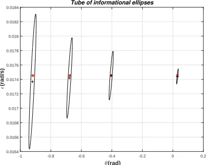
4. Numerical simulation of alignment process
We restrict ourself by the consideration of the simple case of system (0.8) and the procedure of Remark 3. The qualitative sense does not change in the common case.
The following data are used: |θi| ≤ 3 grad, |εi| ≤ 0.1 grad/sec, |ui| ≤ 0.1 rad/sec, T = 100
sec. In integral constraint (0.4) the constants are γi = 0.1 m/sec2. The signal is given byw(t) =
sin(t)/√55. The alignment process is shown on the figures.
5. Conclusion
0 10 20 30 40 50 60 70 80 90 100
t sec
0 0.2 0.4 0.6 0.8 1 1.2
ji
functional, (rad)
Figure 4. Alteration of the functional in the simple model.
-1 -0.8 -0.6 -0.4 -0.2 0 0.2
θ(rad)
0.0164 0.0166 0.0168 0.017 0.0172 0.0174 0.0176 0.0178 0.018 0.0182 0.0184
ǫ
(rad/s)
Tube of informational ellipses
Figure 5. Informational ellipses at the instantst= 44,58,72, and 100.
REFERENCES
1. Lipton A.H.Alignment of Inertial Systems on a Moving Base. Washington D.C.: NASA, 1967. 178 p. 2. Boguslavski I.A.Applied Problems of Filtering and Control. M.: Nauka, 1983. 314 p. [in Russian] 3. Bromberg P.V.The Theory of Inertial Navigation Systems. M.: Nauka, 1979. 245 p. [in Russian] 4. Klimov D.M.Inertial Navigation on the Sea. M.: Nauka, 1984. 211 p. [in Russian]
5. Parusnikov N.A., Morozov V.M, Borzov V.I. Correction Problem in Inertial Navigation. M.: MGU, 1982. 256 p. [in Russian]
6. Bachshiyan B.Ts., Nazirov R.R., Eliyasberg P.E.Determination and Correction of Motion. M.: Nauka, 1980. 402 p. [in Russian]
7. Kurzhanski A.B.Control and Observation under Conditions of Uncertainty. M.: Nauka, 1977. 392 p. [in Russian]
8. Krasovski˘i N.N. and Subbotin A.I. Game-Theoretical Control Problems. Springer–Verlag, New York, 1988. 517 p.
9. Ananyev B.I. and Gredasova N.V. The Alignment Problem of Inertial Systems and
Mo-tion CorrecMo-tion Procedure // Bulletin of Buryatian State University, 2011. No. 9. P. 203–208. old.bsu.ru/content/pages2/1074/2011/AnanevBI.pdf [in Russian]