ISSN 2307-7743 http://scienceasia.asia
_______________
Key words and phrases: Mathematical model; Multi-step differential transform method; Non- standard scheme
© 2013 Science Asia 1 / 19
ANALYTIC NUMERIC SOLUTION FOR SIRC EPIDEMIC MODEL IN FRACTIONAL
ORDER
ANWAR ZEB, GUL ZAMAN, M. IKHLAQ CHOHAN, SHAHER MOMANI, VEDAT SUAT ERTÜRK
Abstract. In this paper, we consider the SIRC (Susceptible-Infected-Recovered-Cross immune) epidemic model. First the non-negative solution of the SIRC model in fractional order is presented. Then the multi-step generalized differential transform method (MSGDTM) is employed to compute an approximation to the solution of the model of fractional order. The obtained results are compared with the results by forth order Runge-Kutta method and nonstandard numerical method in the integer form. Finally, we present some numerical results.
1. Introduction
(removed) individuals who have had the disease and are now immune to the infection (or removed from further propagation of the disease by some other means). These subdivisions of the population are called compartments. To formulate in regular order, the individual goes through consecutive states like S I R,
such models are often called the SIR models.
Two epidemic models: the susceptible-infected-susceptible (SIS) model and the susceptible infected-recovered (SIR) model are commonly used for studying the spreads of epidemics [3,4]. In the SIS epidemic model a recovered individual can be infected again while in the SIR model which assume recovered individuals have lifelong immunity to the disease and this difference makes them suitable for different kinds of infectious diseases. For instance, childhood diseases in which individuals can have long-lasting immunity, either naturally or from vaccination, are appropriate for SIR model. While for viruses transmitting infection, it is more reasonable to use SIS model. Several researchers considered both SIS and SIR epidemic models and presented different epidemics in different regions all over the world [3-5]. Hethcote [6], presented the interaction of susceptible S(t), infected I(t) and recovered R(t) individuals is given by:
( )
( ) ( ) ( ) ( ) ,
( )
( ) ( ) ( ) ( ) ,
( )
( ) ( ) . d S t
N t S t S t I t d t
d I t
S t I t I t
d t d R t
I t R t
d t
Here N(t) is the total population, is the interaction rate of infection, is the death rate
and is the recovery rate. Zaleta and Henandez [7] considered a simple two dimensional
SIS model with vaccination showing backward bifurcation. Casagrandi et al. [9] presented
the SIRC (Susceptible-Infected-Recovered-Cross-immune) model. This compartment (C)
presents an intermediate state between the fully susceptible (S) and the fully protected (R) one. For numerical solutions Jodar et al. [9] presented the nonstandard finite difference schemes. Also Samanta [10] extended the work of Casagrandi et al. [9] for time dependent population size and distributed time delay. But all these work has been done in the integer order differential equations.
example [11-16]. For this purpose Shahed and Alseadi [17] developed a fractional SIRC model. In their work they presented a detailed analysis for the asymptotic stability of disease-free and positive fixed point.
In this paper, we consider an SIRC model. First we show the positive solution of SIRC model in fractional order. Then we use the multi-step generalized differential transform method to approximate the numerical solution. Finally we compare our numerical results with nonstandard numerical method and forth order Runge-Kutta method.
This paper is organized as: In Section 2, we present formulation of the model with some basic definitions and notations related to this work. In Section 3, we show the non-negative solution and uniqueness of the model. In Section 4, the multi-step generalized differential transform method (MSGDTM) is applied to the model. In Section 5, the numerical simulations are presented graphically. Finally, we give conclusion.
2. Formulation of Model with Preliminaries
Here, we consider the model taking by M. El-Shahed et al. [17].
( )
(1 ( ) ) ( ) ( ) ( ) ,
( )
( ) ( ) ( ) ( ) ( ) ( ) ,
( )
(1 ) ( ) ( ) ( ) ( ) ( ) ,
( )
( ) ( ) ( ) ( ) ( ) . d S t
S t I t S t C t d t
d I t
I t S t C t I t I t
d t d R t
C t I t I t R t
d t d C t
R t C t I t C t
d t
(1)
With S( 0 ) S0, I( 0 ) I0, R( 0 ) R0, C( 0 ) C0.
Here is the contact rate of infection, 1 is the cross-immune period, 1 is the infectious period, 1
is the total immune period and is the fraction of the exposed cross-immune individuals who are recruited in a unit time into the infective subpopulation. The total population N t( ) S t( ) I t( ) R t( ) C t( ),
( )
(1 ( ) ) . d N t
N t d t
(2)
Now we introduced fractional order to the system (1) which is consisting of ordinary differential equations. The new system is described by the following set of fractional order differential equations:
( ) (1 ( ) ) ( ) ( ) ( ) , ( 3 )
( ) ( ) ( ) ( ) ( ) ( ) ( ) , ( 4 )
( ) (1 ) ( ) ( ) ( ) ( ) ( ) , ( 5 )
( ) ( ) ( ) ( ) ( ) ( ) , ( 6 )
( ) ( ) . ( 7 )
t
t
t
t
t
D S t S t S t I t C t
D I t S t I t C t I t I t
D R t C t I t I t R t
D C t R t C t I t C t
D N t N t
Here we used the Caputo sense fractional derivative Dt.
Now we give some basic definitions related to this work and fractional calculus [11-16].
Definition A function f( )(x x 0 ) is said to be in the space C( R) if it can be written as for some p where f1( )x is continuous in [ 0 ,), and it is said to be in space
m
C if
( )
, .
m
f C m N
Definition The Riemann-Liouville integral operator of order 0 with a 0 is defined as
1 1
( ) ( ) ( ) ( ) , , ( 8 )
( ) 0
( ) ( ) ( ) . ( 9 )
x
Ja f x a x t f t d t x a
Ja f x f x
Properties of the above operator can be found in [11]. We only need the following:
Definition For f C , a n d fo r , 0 ,a 0 ,c R and 1, we have
( ) ( ) ( ) ( ) ( ) ( ) , (1 0 )
( , 1) , (1 1)
( )
a a a a a
a x a
x
J J f x J J f x J f x
x
J x B
where B ( , 1) is incomplete beta function which is defined as
0
0
1
( , 1) (1 ) , (1 2 )
[ ( ) ]
( ) . (1 3 )
( 1)
k
k c x a c
a
B t t d t
c x a
J e e x a
k
Definition The Caputo fractional derivative of f( )x of order 0 with a 0 is defined as
( ) ( )
1
1 ( )
( ) ( ) ( ) ( ) , (1 4 )
( ) ( ) x a m m m
a a m
f t
D f x J f x d t
x t m
for 1 , , , ( ) 1.
m
m m m N x a f x C
The fractional derivative was investigated by many authors, for m 1 m, f ( )x Cm and 1, we have
1
0
( ) ( )
( ) ( ) ( ) ( ) ( ) . (1 5 )
!
m
k
k
m m k
a a
x a
J D f x J D f x f x f a
k
For mathematical properties of fractional derivatives and integrals one can consult the mentioned references.
3. Non-negative solutions
Let 5 5
{ : 0}
R X R X and ( ) ( ) , ( ) , ( ) , ( ) , ( )
T
X t S t I t R t C t N t . For the proof of the
theorem about non-negative solutions we shall need the following Lemma [16]:
Lemma (Generalized Mean Value Theorem) Let f( )x C a b[ , ] and D f( )x C a b[ , ] for 0 1 .
Then we have, 1
( ) ( ) ( ) ( ) (1 6 )
( )
f x f a D f x a
with 0 x, for all x( , ] .a b
above Lemma that if D f( )x 0 , for all x( 0 , ) ,b then the function f is non-decreasing, and if D f( )x 0 , for all x( 0 , ) ,b then the function f is non-increasing.
Theorem There is a unique solution for the initial value problem given by (3)-(7), and the
solution remains in 5
. R
Proof The existence and uniqueness of the solution of (3)-(7), in ( 0 ,) can be obtained
from [16, Theorem 3.1 and Remark 3.2]. We need to show that the domain 5
R is positively invariant. Since
0
0
0
0
0
| 0 ,
| 0 ,
| (1 ) 0 ,
| 0 ,
| 0 .
S
I
R
C
N
D S C
D I
D R C I I
D C R
D N
On each hyper-plane bounding the nonnegative orthant, the vector field points into 5
. R
4. Multi-step generalized differential transform method.
0 0 0 0( 1 )
( 1 ) (1 ( ) ) ( ) ( ) ( ) ,
( ( 1 ) 1 )
( 1 )
( 1 ) ( ) ( ) ( ) ( ) ( ) ( ) ,
( ( 1 ) 1 )
( 1 )
( 1 ) (1 ) ( ) ( ) ( ) ( ) ( ) , (1 7 )
( ( 1 ) 1 )
( 1 k i k k i i k i k
S k S k S k i I i C k
k k
I k S k i I i C k i I i I k
k k
R k C k i I i I k R k
k C k
0( 1 )
) ( ) ( ) ( ) ( ) ( ) ,
( ( 1 ) 1 )
( 1 )
( 1 ) ( ) .
( ( 1 ) 1 )
k
i
k
R k C k i I i C k
k k
N k N k
k
Here S k( ), I k( ), R k( ),C k( ) and N k( ) are the differential transformation of ( ), ( ), ( ), ( )
S t I t R t C t and N t( ). The differential transform of the initial conditions are
0 0 0 0
( 0 ) , ( 0 ) , ( 0 ) , ( 0 )
S S I I R R C C and N( 0 ) N0.
In view of the differential inverse transform, the differential transform series solution for the system can be obtained as
0 0 0 0 0 ( ) ( ) , ( ) ( ) , ( ) ( ) , ( ) ( ) , ( ) ( ) . K k K k K k K k K k k k k k k
S t S k t I t I k t
R t R k t
C t C k t
N t N k t
(18)
1 1
0
2 1 1 2
0
1 1
0
( ) , [ 0 , ]
( ) ( ) , [ , ] . ( ) . . ( ) ( ) , [ , ] K k K k K
M M M M
k
k
k
k
S k t t t
S k t t t t t
S t
S k t t t t t
(19) 1 1 0
2 1 1 2
0
1 1
0
( ) , [ 0 , ]
( ) ( ) , [ , ] . ( ) . . ( ) ( ) , [ , ] K k K k K
M M M M
k
k
k
k
I k t t t
I k t t t t t
I t
I k t t t t t
(20) 1 1 0
2 1 1 2
0
1 1
0
( ) , [ 0 , ]
( ) ( ) , [ , ] . ( ) . . ( ) ( ) , [ , ] K k K k K
M M M M
k
k
k
k
R k t t t
R k t t t t t
R t
R k t t t t t
(21) 1 1 0
2 1 1 2
0
1 1
0
( ) , [ 0 , ]
( ) ( ) , [ , ] . ( ) . . ( ) ( ) , [ , ] K k K k K
M M M M
k
k
k
k
C k t t t
C k t t t t t
C t
C k t t t t t
1 1
0
2 1 1 2
0
1 1
0
( ) , [ 0 , ]
( ) ( ) , [ , ] . ( ) . . ( ) ( ) , [ , ] K k K k K
M M M M
k
k
k
k
N k t t t
N k t t t t t
N t
N k t t t t t
(23)
Here ( ) , ( ) , ( ) , ( )
j j j j
S k I k R k C k and ( )
j
N k for j 1, 2 , ...,M satisfy the following recurrence relations
0 0 0 0 ( 1)( 1) (1 ( ) ) ( ) ( ) ( ) ,
( ( 1) 1)
( 1)
( 1) ( ) ( ) ( ) ( ) ( ) ( ) ,
( ( 1) 1)
( 1)
( 1) (1 ) ( ) ( ) ( ) (
( ( 1) 1)
k i k k i i k i j j
j j j
j j j j
j j
j j
j
k
S k S k S k i I i C k
k k
I k S k i I i C k i I i I k
k k
R k C k i I i I k
j k
0) ( ) , ( 2 4 )
( 1)
( 1) ( ) ( ) ( ) ( ) ( ) ,
( ( 1) 1)
( 1)
( 1) ( ) .
( ( 1) 1)
k
i
j
j j
j j j
j j
R k
k
C k R k C k i I i C k
k k
N k N k
k
With the initial conditions S j( 0 ) S j1( 0 ) , Ij( 0 ) Ij1( 0 ) , Rj( 0 ) Rj1( 0 ) ,
1
( 0 ) ( 0 ) ,
j j
C C and
1
( 0 ) ( 0 ) .
j j
N N Finally, we start with initial conditions
0 0 0 0 0
( 0 ) , ( 0 ) , ( 0 ) , ( 0 ) ( 0 ) ,
S S I I R R C C a n d N N and use the recurrence
relation given in the above system, we can obtained the multi-step generalized differential transform solution given in (19)-(23).
5. Numerical Method and Simulation
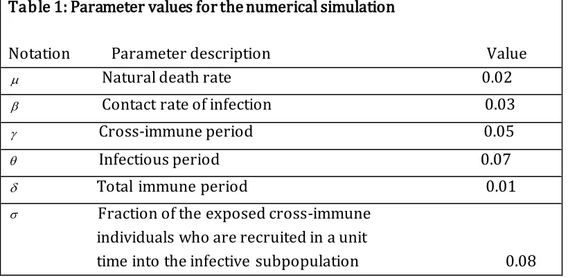
For numerical simulation we use a set of parameters given in Table 1. To demonstrate the effectiveness of proposed algorithm as an approximate tool for solving the nonlinear system of fractional differential equations (3)-(7) for large time t, we apply this algorithm on the interval [0-30].
Table 1: Parameter values for the numerical simulation
Notation Parameter description Value Natural death rate 0.02
Contact rate of infection 0.03 Cross-immune period 0.05
Infectious period 0.07
Total immune period 0.01 Fraction of the exposed cross-immune
individuals who are recruited in a unit
time into the infective subpopulation 0.08
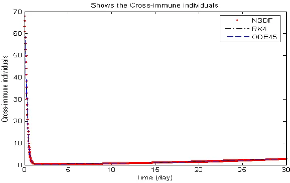
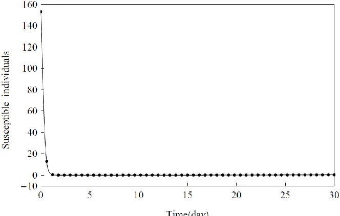
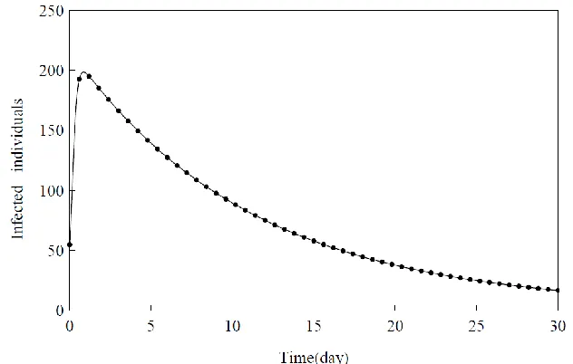
From the graphical results in Figs. 1-5, it can be seen that the results obtained using the multi-step generalized differential transform method match the results of the classical Runge–Kutta method very well, which implies that the presented method can predict the behavior of these variables accurately for the region under consideration.
Fig 1. Shows the susceptible individuals.
Fig. 3. Shows the recovered individuals
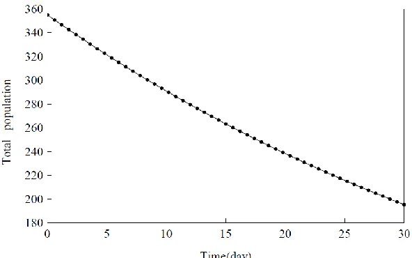
Fig 5. Shows the total time dependent population.
Fig. 7. I(t)versus t: (solid line) MSGDTM, (dotted line) Runge-Kutta method.
Fig. 9. C(t)versus t: (solid line) MSGDTM, (dotted line) Runge-Kutta method.
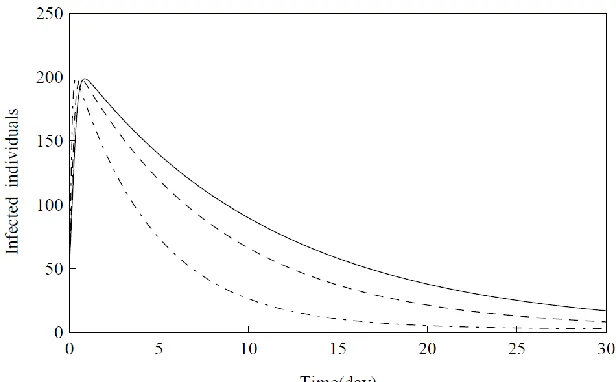
Fig. 11. S(t)versus t: (solid line) 1.0(dashed line) 0.95 , (dot-dashed line) 0.85 .
Fig. 13. R(t)versus t: (solid line) 1.0( dashed line) 0.95 , (dot-dashed line) 0.85 .
Fig. 15. N(t)versus t: (solid line) 1.0( dashed line) 0.95 , (dot-dashed line) 0.85 .
6. Conclusion
In this paper, a fractional order system for SIRC
(Susceptible-Infected-Recovered-Cross-immune) epidemic model is studied and its approximate solution is presented using the multi-step generalized differential transform method (MSGDTM).
The approximate solution obtained by multi-step generalized differential transform method are highly accurate and valid for a long time in the integer case. This method is very applicable and also this is a good approach for the solutions of differential equations of such order.
This tool is the best one for modeling in science and engineering.
REFERENCES
[1] P. Roumagnac, F.X. Weill, C. Dolecek, S. Baker, S. Brisse, N.T. Chinh, T.A.H. Le, C.J. Acosta, J. Farrar, G. Dougan, M. Achtman, Evolutionary history of salmonella typhi, Science, 314 (2006)1301-1304.
[2] W.O. Kermack, A.G. McKendrick “Contributions to the mathematical theory of epidemics, part 1” Proc. Roy. Soci. Edin. Sec. A. Math., 115 (1927) 700-721.
[3] B. Shulgin, L. Stone, Z. Agur “Pulse vaccination strategy in the SIR epidemic model” Bull. Math. Biol., 60 (1998)1123-1148.
[4] G. Zaman, Y.H. Kang, I.H. Jung “Stability analysis and optimal vaccination of an SIR epidemic model”
ScienceDirect, BioSys., 93 (2008) 240-249.
[5] A.A. Lashari, G. Zaman “Global dynamics of vector-borne diseases with horizontal transmission in host population” Comp. Math. Appl., 61 (2011) 745-754
[6] H.W. Hethcote, Qualitative analysis of communicable disease model, Math. Biosci, 7 (1976) 335-356. [7] M.I. Kamien, N.L. Schwartz, Dynamics Optimization:The Calculus of Variations and Optimal Control in
[8] C.M. Kribs-Zaleta, J.X. Velasco-Hernandez, A simple vaccination model with multiple endemic states, Math. Biosci, 164 (2000) 183-201.
[9] R. Casagrandi, L. Bolzoni, S.A. Levin, V. Andreasen, The SIRC model for influenza A, Math. BioSci, 200 (2006) 152-169.
[10] I. Podlubny, Fractional Differential Equations, Academic Presss, London, 1999.
[11] V.S. Erturk, Z.M. Odibait, S. Momani, An approximate solution of a fractional order differential equation model of human T-cell lymphotropic virus I (HTLV -I) infection of CD4 T-cells, Computers &
Mathematics with applications, 62 (3)(2011) 996-1002.
[12] S. Miller, B. Ross, An Introduction to the Fractional Calculus and Fractional Differential Equations, Willey, New York, 1993.
[13] E. Ahmed, A.M.A. El-Sayed, H.A.A. El-Saka, Equilibrium points, stability and numerical solutions of fractional-order predator-prey and rabies models, JMAA, 325 (2007) 542-553.
[14] N. Ozalp, E. Demirci, A fractional order SEIR model with vertical transmission, Mathematical and Computer modeling 54 (2011) 1-6.
[15] Z.M. Odibat, N.T.Shawafeh, Generalized Taylor's formula, Comput. Math. Appl. 186 (2007) 286-293. [16] W. Lin, Global existence theory and chaos control of fractional differential equations, JMAA, 332 (2007) 709-726.
[17] M. El-Shahed, A. Alseadi, The fractional SIRC model and influenza A, Mathematical Problems in Engineering, (2011) ID 480378.
ANWAR ZEB, DEPARTMENT OF MATHEMATICS, UNIVERSITY OF MALAKAND, CHAKDARA DIR (LOWER), KHYBER PAKHTUNKHAWA, PAKISTAN
GUL ZAMAN*, DEPARTMENT OF MATHEMATICS, UNIVERSITY OF MALAKAND, CHAKDARA DIR (LOWER),
KHYBER PAKHTUNKHAWA, PAKISTAN
M. IKHLAQ CHOHAN, DEPARTMENT OF BUSİNESS ADMİNİSTRATİON AND ACCOUNTİNG, BURAİMİ UNİVERSİTY, COLLEGE, AL-BURAİMİ, OMAN
SHAHER MOMANİ, THE UNIVERSITY OF JORDAN, FACULTY OF SCIENCE, DEPARTMENT OF MATHERMATICS, AMMAN 1194, JORDAN
VEDAT SUAT ERTÜRK, DEPARTMENT OF MATHEMATICS, FACULTY OF ARTS AND SCIENCES, ONDO KUZ MAYIS UNIVERSITY, 55139, SAMSUN, TURKEY