Available online throug
ISSN 2229 – 5046
NUMERICAL SOLUTION OF THE FRACTIONAL
KORTEWEG–DE VRIES (KdV) EQUATION BY q-HOMOTOPY ANALYSIS METHOD (q-HAM)
Dr. ANOOP KUMAR*
School of Basic and Applied Sciences,
Central University of Punjab Bathinda (CUPB),
in Centre for Mathematics & Statistics, India
(Received On: 24-07-17; Revised & Accepted On: 16-08-17)
ABSTRACT
In this paper, we consider the fractional Korteweg–de Vries (KdV) equation. A relatively new method called the
q-homotopy analysis method (q-HAM) is adopted to obtain an analytical solution of the fractional Korteweg–de Vries (KdV) equation in series form. Our analysis shows the simplicity nature of the application of q-HAM to nonlinear fractional differential equations. The convergence rate of the method used is faster in the sense that just very few terms of the series solution are needed for a good approximation due to the presence of the auxiliary parameter h comparable to exact solutions. Numerical solution obtained by this method is compared with the exact solution. Our error analysis shows that the analytical solution converges very rapidly to the exact solution. Numerical results are obtained using the software Mathematica.Keywords: q-homotopy analysis method (q-HAM), fractional Korteweg–de Vries (KdV) equation, approximate numerical solutions, symbolic computation.
1. INTRODUCTION
In recent decades, fractional calculus has found diverse applications in different scientific and technological fields [1, 2], such as thermal engineering, acoustics, electromagnetism, control, robotics, viscoelasticity, diffusion, edge detection, turbulence, signal processing, information sciences, communications, and many other physical processes and also in medical sciences. Fractional differential equations (FDEs) have also been applied in modeling many physical and engineering problems and fractional differential equations in nonlinear dynamic [3]. The importance of getting approximate and exact solutions of nonlinear fractional differential equations in mathematics and physics remains an important problem that requires the discovering new methods of approximate and exact solutions. However, finding the exact solutions to these non-linear fractional differential equations are difficult to obtain it [4]. Therefore, the numerical methods used to deal with these equations [5] and they have largely been using some semi analytical techniques to solve these equations such as, differential transform method [6, 7, 8], Laplace decomposition method [9], homotopy perturbation method [10], variational iteration method [11, 12] and homotopy analysis method (HAM) [13, 14, 15]. The HAM initially proposed by Liao in his Ph.D. and thesis [13] is a powerful method to solve the non-linear problems. In recent years, this method has been successfully employed to solve many types of non-linear problems in science and engineering [16, 17, 18]. The HAM contains a certain auxiliary parameter ℎ, which provides us with a simple way to adjust and control the convergence region and the rate of convergence of the series solution. Many workers applied the HAM to solve fractional differential equations [19, 20]. El-Tawil and Huseen [21] established a method namely q-homotopy analysis method (q-HAM) which is a more general method of HAM, The q-HAM contains an auxiliary parameter
n
as well ash
such that the case ofn
=
1
(q-HAM;n
=
1
) the standard homotopy analysis method (HAM) can be reached. In this paper, we have applied the q-homotopy analysis method (q-HAM) [22, 23] to solve the fractional Korteweg–de Vries (KdV) equation [24] with given initial condition. The main advantage of the method is the fact that it provides its user with an analytical approximation solution, in a rapidly convergent series with elegantly computed terms. The structure of this paper is organized as follows:In section 2, we begin with the basic definition of Caputo’s fractional derivative. In section 3, we give the basic concept of the q-homotopy analysis method (q-HAM). In section 4, we apply this method to solve the fractional Korteweg– de Vries (KdV) equation with given initial condition.
2. PRELIMINARIES
This section is devoted to some definitions and some known results. Caputo’s fractional derivative is adopted in this work.
Definition 2.1: The Riemann-Liouville’s (RL) fractional integral operator of order
α
≥
0
,
of a functionf
∈
L
1(
a
,
b
)
is given as
(
)
∫
−
>
>
Γ
=
t −t
d
f
t
t
f
I
0 1,
0
,
0
,
)
(
)
(
1
)
(
τ
τ
τ
α
α
α α
(1)
where
Γ
is the Gamma function andI
0f
(
t
)
=
f
(
t
).
Definition 2.2: The fractional derivative in the Caputo’s sense is defined as [4]
(
)
∫
− − −−
−
Γ
=
=
t n n n nd
f
t
n
t
f
D
I
t
f
D
0 ) ( 1,
)
(
)
(
1
)
(
)
(
τ
τ
τ
α
α α α (2)0
,
,
1
<
≤
∈
Ν
>
−
n
n
t
n
where
α
Lemma 2.1: Let
t
∈
(
a
,
b
].
Then[
]
(
)
,
0
,
0
.
)
1
(
)
1
(
)
(
)
(
−
≥
>
+
+
Γ
+
Γ
=
−
+α
β
α
β
β
β αβ α
a
t
t
a
t
I
(3)3. BASIC CONCEPTS OF Q-HOMOTOPY ANALYSIS METHOD
Considering the following differential equation of the form:
,
0
)
,
(
)]
,
(
[
D
u
x
t
−
f
x
t
=
N
tα (4)where
N
is a nonlinear operator,D
tαdenote the Caputo’s fractional derivative,u
(
x
,
t
)
is an unknown function,x
and
t
denote the space and time variables andf
(
x
,
t
)
is a known function, respectively. To generalize the original homotopy method, the zeroth-order deformation equation is constructed as)),
,
(
)]
;
,
(
[
(
)
,
(
]
)
,
(
)
;
,
(
[
)
1
(
−
nq
L
ϕ
x
t
q
−
u
0x
t
=
q
H
x
t
N
D
tαϕ
x
t
q
−
f
x
t
(5)where
∈
≥
n
q
n
1
,
0
,
1
denotes the so called embedding parameter,
≠
0
is a non-zero auxiliary parameter,)
,
(
x
t
H
is a non-zero auxiliary function,L
is an auxiliary linear operator,u
0(
x
,
t
)
is an initial guess ofu
(
x
,
t
)
and)
;
,
(
x
t
q
ϕ
is an unknown function. It is important to note that one has great freedom to choose the auxiliary things inq-HAM. Clearly, when
q
=
0
and1
,
n
q
=
it holds that:and
t
x
u
t
x
,
;
0
)
(
,
)
(
=
0ϕ
1
, ;
( , ).
x t
u x t
n
φ
=
(6)Thus, as
q
increases from 0 ton
1
, the solution
ϕ
(
x
,
t
;
q
)
varies from the initial guessu
0(
x
,
t
)
to the solution).
,
(
x
t
u
Ifu
0(
x
,
t
),
L
,
h
,
H
(
x
,
t
)
are chosen approximately, the solutionϕ
(
x
,
t
;
q
)
of equation (5) existsfor
∈
n
q
0
,
1
. Expandingϕ
(
x
,
t
;
q
)
in Taylor’s series aboutq
=
0
,
we have:,
)
,
(
)
,
(
)
;
,
(
1 0∑
∞ =+
=
m m mx
t
q
u
t
x
u
q
t
x
ϕ
(7)where
(
,
;
)
.
!
1
)
,
(
0 =∂
∂
=
q m m mq
q
t
x
m
t
x
We suppose that the auxiliary linear operator L, the initial guess
u
0,
the nonzero auxiliary functionH
(
x
,
t
)
and thenonzero auxiliary parameter
are properly chosen such that the above series (7) converges at1
,
n
q
=
and then wehave:
,
1
)
,
(
)
,
(
)
1
;
,
(
)
,
(
1 0∑
∞ =
+
=
=
m m mn
t
x
u
t
x
u
n
t
x
t
x
u
ϕ
(9)which must be one of the solutions of the original non-linear differential equation. Let the vector
u
nbe defined as follows:)}.
,
(
...,
),
,
(
),
,
(
),
,
(
{
u
0x
t
u
1x
t
u
2x
t
u
x
t
u
n=
n (10)Differentiating the equation (5), m-times with respect to the (embedding) parameter
q
, then evaluating atq
=
0
and finally dividing them bym
!
throughout, we obtain the m-th order deformation equation (Lioa [13]) as:))
,
(
(
)]
,
(
)
,
(
[
u
x
t
*u
1x
t
H
R
u
1x
t
L
m m m m m→ −
−
=
−
χ
(11) with initial conditionsu
m(k)(
x
,
t
)
=
0
,
k
=
0
,
1
,
2
,
3
,...,
m
−
1
0 1 1 1
))
,
(
)]
;
,
(
[
(
)!
1
(
1
))
,
(
(
= − − → −∂
−
∂
−
=
q m t m m mq
t
x
f
q
t
x
D
N
m
t
x
u
R
ϕ
α (12) and
≤
=
.
,
,
1
,
0
*otherwise
n
m
mχ
(13)3.1. Remark: It should be emphasized that
u
m(
x
,
t
)
for
m
≥
1
is governed by the linear operator (11) with the linearboundary conditions that come from the original problem. The existence of the factor
m
n
1
, more chances for
convergence may occur or even much faster convergence can be obtained better than the standard HAM. It should be noted that the cases of
(
n
=
1
)
in equation (5), the standard HAM can be reached.4. APPROXIMATE SERIES SOLUTION OF THE PROBLEM
In this section, we shall apply the q-HAM to obtain the series solution of the fractional Korteweg–de Vries (KdV) equation with given initial condition.
4.1. THE FRACTIONAL KORTEWEG-DE VRIES (KDV) EQUATION:
We first consider the fractional Korteweg–de Vries (KdV) equation given by [24] as,
,
1
0
,
0
,
0
6
+
=
>
<
≤
+
α
αt
u
uu
u
D
t x xxx (14)with initial conditions
.
2
2
1
)
0
,
(
2
=
Sech
x
x
u
(15)The true solutions for
α
=
1
of the equation (14) which is obtained by the MFRDTM [24]is given by.
2
2
1
)
,
(
x
t
=
Sech
2
−
x
t
u
(16)Let us now solve the equation (14) by the q-homotopy analysis method (q-HAM).
We choose the linear noninteger order operator as:
),
;
,
(
)]
;
,
(
[
x
t
q
D
x
t
q
L
ϕ
=
tαϕ
(17)with the property
L
(
c
1)
=
0
,
wherec
1 is constant. Also, we use
=
2
2
1
)
0
,
(
x
Sech
2x
u
as the initialapproximation. From the equation (15), we define the non-linear fractional partial differential operator as:
).
;
,
(
)
;
,
(
)
;
,
(
6
)
;
,
(
)]
;
,
(
[
x
t
q
D
x
t
q
x
t
q
x
t
q
x
t
q
Using the above definitions, we construct the zero-order deformation equation:
)].
;
,
(
[
)
,
(
)]
,
(
)
;
,
(
[
)
1
(
−
nq
L
ϕ
x
t
q
−
u
0x
t
=
q
H
x
t
N
ϕ
x
t
q
(19)Choosing the
H
(
x
,
t
)
=
1
,
we define the mth-order deformation equation as:)),
,
(
(
)]
,
(
)
,
(
[
1 1*
t
x
u
R
t
x
u
t
x
u
L
m m m m m→ −
−
=
−
χ
(20) with the initial condition form
≥
1
,
u
m(
x
,
0
)
=
0
,
where
≤
=
otherwise
n
m
m,
,
1
,
0
*χ
and.
))
,
(
(
))
,
(
(
)
,
(
6
)
,
(
))
,
(
(
1 11
0 1
1 m j x m xxx
m j j m t m
m
u
x
t
D
u
x
t
u
x
t
u
x
t
u
x
t
R
−− −−
= −
→
−
=
α+
∑
+
(21)Now the solution of equation (20), for
m
≥
1
becomes))].
,
(
(
[
)
,
(
)
,
(
x
t
*u
1x
t
L
1R
u
1x
t
u
m m m m m→
− −
−
+
=
χ
(22) It is straightforward to choose the initial approximationu
0(
x
,
t
)
=
u
(
x
,
0
)
which is given by the equation (15). Therefore, using the q-HAM, we obtain the components of the solution successively as follows.We, therefore, obtain:
,
2
2
1
)
0
,
(
2
=
Sech
x
x
u
]
)
(
)
(
6
[
)
,
(
0 0 0 01
x
t
D
tD
tu
u
u
xu
xxxu
=
−α α+
+
[ ]
,
)
1
(
2
4
]
)
(
)
(
6
[
4 3 0 0 0 0+
Γ
−
=
+
+
=
α
α αα
x
t
Sinh
x
Csch
u
u
u
u
D
I
t t x xxx
(23)]
)
(
)
(
6
)
(
6
[
)
,
(
1 1 0 1 1 0 12
x
t
n
u
D
tD
tu
u
u
xu
u
xu
xxxu
=
+
−α α+
+
+
=
n
u
1+
I
tα[
D
tαu
1+
6
u
0(
u
1)
x+
6
u
1(
u
0)
x+
(
u
1)
xxx]
[ ]
[
]
)
1
2
(
2
]
[
2
4
)
1
(
2
)
(
4
2 4 2 4 3+
Γ
+
−
+
+
Γ
+
−
=
α
α
α αt
x
Sech
x
Cosh
t
x
Sinh
x
Csch
n
, (24)]
)
(
)
(
6
)
(
6
)
(
6
[
)
,
(
2 2 0 2 1 1 2 0 23
x
t
n
u
D
tD
tu
u
u
xu
u
xu
u
xu
xxxu
=
+
−α α+
+
+
+
]
)
(
)
(
6
)
(
6
)
(
6
[
2 0 2 1 1 2 0 22
I
tD
tu
u
u
xu
u
xu
u
xu
xxxu
n
+
+
+
+
+
=
α α
[ ]
(
)
)
1
2
(
2
]
[
2
2
)
(
)
1
(
2
)
(
4
2 4 2 4 3 2+
Γ
+
−
+
+
+
Γ
+
−
=
α
α
α αt
x
Sech
x
Cosh
n
t
x
Sinh
x
Csch
n
[ ]
)
1
3
(
2
2
16
57
)
1
3
(
2
2
8
3 7 3 3 6 3 3+
Γ
−
+
Γ
−
α
α
α αt
x
Sinh
x
Sech
t
x
Tanh
x
Sinh
x
Csch
[ ]
.
)
1
3
(
2
5
2
32
3
)
1
3
(
2
3
32
27
7 3 3 7 33
+
Γ
−
+
Γ
+
α
α
α αt
x
Sinh
x
Sech
t
x
Sinh
x
Sech
(25)From the equations (23), (24) and (25), we obtain
u
1(
x
,
t
),
u
2(
x
,
t
)
and
u
3(
x
,
t
)
similarly by puttingm
=
4
,
5
,
...
in equation (22), we can obtain
u
i(
x
,
t
),
i
≥
4
by using the Methematica. Therefore, the four-terms approximate seriessolution to the problem (14) in terms of convergence parameter
h
and
n
is given by4.2. Remark: It should be emphasized that
u
m(
x
;
t
)
form
>
1
, is governed by the linear operator (7) with the linearboundary conditions that come from the original problem. The existence of the factor
i
n
1
gives more chances for
better convergence, faster that the solution obtained by the standard HAM. Of course, when
n
=
1
,
we are in the case of the standard HAM.4.3. The h-curve:
The question that comes to the mind when the following this method of solution is how one chooses the auxiliary parameter h to get a good approximate solution. The answer is in the h-curve. Apparently, our choice in the plots can be seen directly from the graph, the range of which is by drawing a horizontal line on the curve parallel to x-axis. Fig. 1 is made with
n
=
1
,
and
α
=
1
.
Figure-1: The h-curve of
u
(
x
,
t
,
n
,
h
)
of the four-terms approximate series solution of the equation (26) obtained by q-HAM for fixed the value ofn
=
1
,
and
α
=
1
.
5. NUMERICAL ANALYSIS
In this section, we give some numerical results using series solution obtained above. Comparison is made with the exact solution for a special case using the four-terms series solution. We also seen the graph displaying the best choice of h for fast convergence and the effects of different fractional order
α
on the solution obtained.5.1. Comparison of the approximate solution with exact solution
Exact solution is known in the case of
α
=
1
and so we present the numerical result (four-terms series solution) obtained by the q-homotopy analysis method and the exact solution of equation the (14) under some conditions.0.1 0.2 0.3 0.4 0.5 t
0.30 0.35 0.40 0.45 0.50
u
x, t
Figure-2: The seven-terms approximation solution of the q-HAM plot of
u
(
x
,
t
)
forh
=
0
.
88
,
n
=
1
andα
=
1
against the exact solution obtained by MFRDTM.
h-curve
x-axis
q-HAM
(a) (b)
Figure-3: Fig. 3(a) is the exact solution (16) obtained by MFRDTM and fig. 3(b) is the four-terms approximate series solution (26), obtained by the q-HAM for
h
=
−
0
.
95
,
n
=
1
,
α
=
1
.
5.2. Remark: It should be noted that we have used only the four-terms of the series solution obtained by the q-homotopy analysis method to make fig.2 as against the solution obtained by the modified fractional reduced differential transform method [MFRDTM]. Fig.2 and 3 shows a perfect match with exact solution. This shows the effectiveness of the homotopy analysis method over other analytical methods due to the ability to control or choose appropriately the auxiliary parameter h.
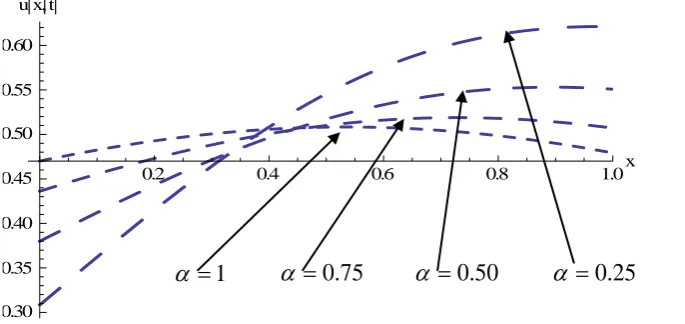
5.3. Solution plots with different fractional values of
α
Here, we give the solution plots of the four-terms series solution (26) of the equation (14) using the MATHEMATICA obtained by q-homotopy analysis method (q-HAM). This shows the effect of the different fractional values of
α
on the obtained solution (26) in figure 4 and 5.0.2 0.4 0.6 0.8 1.0t
0.30 0.35 0.40 0.50 0.55 0.60 0.65
u
x,t
Figure-4: The q-HAM solution plot of Eq. (14) for different fractional values of
α
with fixed.
1
88
.
0
,
75
.
0
=
−
=
=
h
and
n
x
50
.
0
=
α
75
.
0
=
α
1
=
α
=
1
α
=
0
.
25
0.2 0.4 0.6 0.8 1.0x
0.30 0.35 0.40 0.45 0.50 0.55 0.60
u
x, t
Figure-5: The q-HAM solution plot of Eq. (14) for different fractional values of
α
with fixed.
1
88
.
0
,
5
.
0
=
−
=
=
h
and
n
t
Table-1: Absolute errors for u(x, t) obtained by the four-terms approximate series solution (26) the equation (14) obtained the q-HAM against with the exact solution obtained by MFRDTM [24] for
n
=
1
and
h
=
−
0
.
95
t x
α
=
1
α
=
0
.
75
α
=
0
.
50
α
=
0
.
25
.01
-3 -2 -1 0 1 2 3
6.4341854E-8 1.4465059E-7 1.7481382E-7 0.0000000 1.2350665E-7 2.0084081E-7 1.1208361E-7
1.9513911E-3 3.8500738E-3 4.4864765E-3 0.0000000 4.3880173E-3 3.9583612E-3 2.0431764E-3
7.8501271E-3 1.576909E-2 1.9548745E-2 0.0000000 1.8153032E-2 1.7302939E-2 9.1512339E-3
2.4518746E-2 4.9665235E-2 7.7083517E-2 0.0000000 6.1261918E-2 6.7066096E-2 3.9267895E-2
.02 -3 -2 -1 0 1 2 3
3.1070078E-9 7.1011681E-8 6.6448348E-8 0.0000000 2.7269763E-7 2.9403599E-7 1.8776022E-7
2.9774284E-3 5.9132759E-3 7.0280876E-3 0.0000000 6.7578813E-3 6.2104572E-3 3.2293205E-3
1.0377445E-2 2.1049732E-2 2.7218635E-2 0.0000000 2.4441339E-2 2.4104253E-2 1.2966486E-2
2.8903930E-2 5.7875504E-2 9.5709924E-2 0.0000000 7.3353075E-2 8.2463946E-2 4.9745348E-2
.03 -3 -2 -1 0 1 2 3
2.8630366E-7 3.8130087E-7 1.1900928E-6 0.0000000 1.6579801E-6 1.1399201E-7 1.4277332E-7
3.7519086E-3 7.4954524E-3 9.0750797E-3 0.0000000 8.5903517E-3 8.0285838E-3 4.2037871E-3
1.2071311E-2 2.4649702E-2 3.2995673E-2 0.0000000 2.8850929E-2 2.9208179E-2 1.5935114E-2
3.1876547E-2 6.3103487E-2 1.0897626E-1 0.0000000 8.1623805E-2 9.3186198E-2 5.7374956E-2
.04 -3 -2 -1 0 1 2 3
8.6912112E-7 1.3709774E-6 3.6612943E-6 0.0000000 4.5026128E-6 5.0666361E-7 1.0724971E-7
4.3796942E-3 8.7973092E-3 1.0843835E-2 0.0000000 1.0112703E-2 9.6014813E-3 5.0612894E-3
1.3351203E-2 2.7397237E-2 3.7816055E-2 0.0000000 3.2318003E-2 3.3444148E-2 1.8476598E-2
3.4200079E-2 6.6967149E-2 1.1964957E-2 0.0000000 8.8105309E-2 1.0166012E-2 6.3606173E-2
.05 -3 -2 -1 0 1 2 3
1.8353558E-6 3.0550361E-6 7.9440418E-6 0.0000000 9.2777139E-6 1.7371032E-6 6.4680586E-7
4.9067225E-3 9.9061081E-3 1.2426918E-2 0.0000000 1.1423800E-2 1.1009503E-2 5.8418999E-3
1.4377785E-2 2.9611832E-2 4.2039288E-2 0.0000000 3.5202075E-2 3.7131662E-2 2.0751599E-2
3.6139437E-2 7.0027067E-2 1.2873086E-2 0.0000000 9.3513577E-2 1.0875979E-2 6.8969615E-2
A very good agreement between the results of the q-HAM and the exact solutions is observed in Figures 2, 3 and Table 1, which confirms the validity of the q-HAM.
25
.
0
=
α
50
.
0
=
α
75
.
0
=
α
1
6. CONCLUSION
In this paper, we have successfully applied q-homotopy analysis method (q-HAM) to obtain an approximation of the analytic solution of the fractional Korteweg–de Vries (KdV) equation. In this method, the solution is found in the form of a convergent series with easily computed terms. The results obtained by the q-homotopy analysis method (q-HAM) are compared with the modified fractional reduced differential transform method (MFRDTM) solution, which show a very good agreement, even using only few terms of the recursive relations. In general, this method provides highly accurate numerical solutions and can be applied to a wide class of nonlinear problems. Also, the method avoids
linearization and physically unrealistic assumptions. The results demonstrate reliability and efficiency of the q-homotopy analysis method (q-HAM). The fact that this technique solves the linear and nonlinear problems can be
considered as a clear advantage of this algorithm over the decomposition method. Finally, we conclude that the q-HAM can be considered as a nice refinement in existing numerical techniques and have wide applications in different fields of sciences.
7. ACKNOWLEDGEMENT
The authors, Dr. Anoop Kumar is highly thankful to the Central University of Punjab bathinda (CUPB), Punjab, India for the financial support from the University Research Seed Money (RSM) grant and all the necessary facility. The author also would like to express their sincere thanks to the Professor Dr. Rajan Arora, Department of Applied Science and Engineering, I.I.T. Roorkee, Roorkee, for his valuable motivation and suggestions.
REFERENCES
1. F. Mainardi, “Fractional calculus: some basic problems in continuum and statistical mechanics,” in Fractals and Fractional Calculus in Continuum Mechanics, vol. 378, pp. 291–348, Springer, New York, USA, 1997. 2. M. Dalir and M. Bashour, “Applications of fractional calculus,” Applied Mathematical Sciences, vol. 4,
no. 21–24, pp. 1021–1032, 2010.
3. H. Jafari and V. Daftardar-Gejji, “Solving a system of non-linear fractional differential equations using Adomian decomposition,” Journal of Computational and Applied Mathematics, vol. 196, no. 2, pp. 644–651, 2006.
4. Y. Q. Liu and J. H. Ma, “Exact solutions of a generalized multi-fractional nonlinear diffusion equation in radical symmetry,” Communications in Theoretical Physics, vol. 52, no. 5, pp. 857– 861, 2009.
5. Z. A. Anastassi and T. E. Simos, “Numerical multistep methods for the efficient solution of quantum mechanics and related problems,” Physics Reports, vol. 482-483, pp. 1–240, 2009.
6. Z. Odibat, S. Momani, and V. S. Erturk, “Generalized differential transform method: application to differential equations of fractional order,” Applied Mathematics and Computation, vol. 197, no. 2, pp. 467–477, 2008. 7. A. K. Alomari, “A new analytic solution for fractional chaotic dynamical systems using the differential
transform method,” Computers & Mathematics with Applications, vol. 61, no. 9, pp. 2528-2534, 2011.
8. J. Liu and G. Hou, “Numerical solutions of the space- and time fractional coupled Burgers equations by generalized differential transform method,” Applied Mathematics and Computation, vol. 217, no. 16, pp. 7001-7008, 2011.
9. Arora R. and Kumar A., Solution of Linear and Nonlinear PDEs by the He’s Variational Iteration Method, Recent Advances in Intelligent Control, Modelling and Computational Science, ISBN: 978-960-474-319-3, pp. 15-19, (2013).
10. H. Jafari, C. M. Khalique, and M. Nazari, “Application of the Laplace decomposition method for solving linear and nonlinear fractional diffusion-wave equations,” Applied Mathematics Letters, vol. 24, no. 11, pp. 1799-1805, 2011.
11. S. Momani and Z. Odibat, “Homotopy perturbation method for nonlinear partial differential equations of fractional order,” Physics Letters A, vol. 365, no. 5-6, pp. 345-350, 2007.
12. Y. M. R, M. S. M. Noorani, and I. Hashim, “Variational iteration method for fractional heat- and wave-like equations,” Nonlinear Analysis: Real World Applications, vol. 10, no. 3, pp. 1854-1869, 2009.
13. Liao SJ. “On the homotopy analysis method for nonlinear problems,” Appl Math Comput, 147, pp. 499-513, 2004.
14. Liao SJ. “Comparison between the homotopy analysis method and homotopy perturbation method,” Applied Mathematics and Computation, 169, pp. 1186-1194, 2005.
15. Arora R. and Kumar A., Solution of the Coupled Drinfeld’s–Sokolov–Wilson (DSW) System by Homotopy Analysis Method, Advanced Science, Engineering and Medicine, vol. 5, pp. 1–7, 2013.
16. Molabahrami A. and Khani F. “The homotopy analysis method to solve the Burgers– Huxley equation,” Nonlinear Analysis: Real World Applications, 1, pp. 589-600, 2009.
17. Noor M. A., “Iterative methods for nonlinear equations using homotopy perturbation technique,” Applied Mathematics & Information Sciences, vol. 4, no. 2, pp. 227-235, 2010.
19. Song L. and Zhang H. “Application of homotopy analysis method to fractional KdV- Burgers–Kuramoto equation,” Phys Lett A, 2007.
20. S. T. Mohyud-Din, A. Yildirim and M. Usman, “Homotopy analysis method for fractional partial differential equations,” International Journal of the Physical Sciences, Vol. 6(1), pp. 136-145, 2011.
21. El-Tawil M. A. and Huseen S. N., “The q-Homotopy Analysis Method (q-HAM),” International Journal of Applied mathematics and mechanics, 8 (15), pp. 51-75, 2012.
22. El-Tawil M. A. and Huseen S. N., “On Convergence of The q-Homotopy Analysis Method,” Int. J. Contemp. Math. Sciences, Vol. 8, no. 10, pp. 481-497, 2013.
23. Iyiola O. S. “q-Homotopy Analysis Method and Application to Fingero-Imbibition phenomena in double phase flow through porous media,” Asian Journal of Current Engineering and Maths, 2, pp. 283-286, 2013. 24. S. Saha Ray, “Numerical solutions and solitary wave solutions of fractional KdV equations using modified
fractional reduced differential transform method,” Computational Mathematics and Mathematical Physics, vol. 53, no. 12, pp.1870–1881, 2013.
Source of support: Nil, Conflict of interest: None Declared.