Vol 7, No 8 (2016)

(1)

Available online through

ISSN 2229 – 5046

International Journal of Mathematical Archive- 7(8), August – 2016 53

APPLICATION OF HAAR WAVELET COLLOCATION METHOD

TO SOLVE THE FIFTH ORDER ORDINARY DIFFERENTIAL EQUATIONS

A. PADMANABHA REDDY

1,*

_{, C. SATEESHA}

2

_,

_{MANJULA S. H.}

3

1, 2, 3._{Department of Studies in Mathematics,} V. S. K. University, Ballari-583104, Karnataka, India.

(Received On: 29-07-16; Revised & Accepted On: 10-08-16)

ABSTRACT

A

method based on Haar wavelets is proposed for the numerical solution of fifth order ordinary differential equations. In order to demonstrate the applicability and efficiency of this method five test problems are considered, few of them are chosen from the field of viscoelastic flows. Superiority of this method has been studied through the comparison of various techniques available in the literature.

Keywords: Haar wavelets, Fifth order ordinary differential equations, Quasilinearization technique, Collocation

method.

Mathematics Subject Classification: 32G34, 65T60.

INTRODUCTION

The applications of wavelet have been occurred in various forms since the beginning of twentieth century viz. Calderon-Zygmund theory and Littlewood-Paley technique in harmonic analysis and digital filter bank theory in signal/image processing. However, in its present form due to multiresolution analysis wavelet theory attracted various disciplines such as numerical analysis, chemical engineering, data compression, medical imaging etc [1]. Wavelet technique enables us to decompose a complicated function into several simpler ones and study them independently. The success history of digitizing fingerprints by FBI using biorthonormal spline wavelets, manufacturing of chips for JPEG 2000, finer structure analysis of electrocardiograph (ECG) using wavelet families are the attractive fields of science and technology [2].

In recent years wavelet based algorithms are becoming popular in the field of numerical analysis because of the properties of localization. Wavelet based method of different families such as Daubechies, Coiflet, Biorthogonal Spline, Symlet wavelets etc are developed for the numerical solution of problems which can be modeled with the help of differential or integral equations occur in various disciplines. A disadvantage of these wavelet families is that they do not have an explicit expression for scaling or wavelet function. As a result we will have complicated process for the integration or differentiation of these wavelets. Among the wavelet families which have an analytic expression mathematically simplest are the Haar wavelets. Alfred Haar [3] introduced the notion of wavelets and they placed a crucial role for the numerical solution of differential or integral equations [4]. At present there are two approaches to applying the Haar wavelet for integrating ordinary differential equations (ODE). In case of the first method for integrating ODE concept of operational matrix is introduced by Chen and Hsiao [5, 6]. Another approach is called direct method due to Lepik [7]. In this approach Haar functions are integrated directly. The direct method is easily applicable for calculating integrals of arbitrary order but the operational matrix method has been used mainly for first order integrals. Harpreet Kaur et al. [8] solved boundary value problems (BVPs) by Haar wavelet collocation method (HWCM) and utilized quasilinearization tecnique to resolve quadratic nonlinearity in dependent variable. Siraj-ul-Islam et al. [9] found the numerical solution of second order BVPs by collocation method with the Haar wavelets. Fazal-i-Haq et al. [10 -12] solved fourth, sixth and eighth order BVPs from various disciplines by using Haar wavelets. Reddy et al. [13] have demonstrated the superiority of the HWCM for the solution seventh order ODEs which occur in the modeling of induction motors with two rotor circuits. Saha Ray et al. [14-15] have implemented Haar wavelet method for the solution of equations occur in partial differential equations and fractional calculus. The several applications of Haar wavelet method can be found in the survey article by Hariharan and Kannan [16].

Corresponding Author: A. Padmanabha Reddy1,*

(2)

The BVPs are widely used in Mathematics, Physics and Engineering Sciences. In the Mathematical modeling of viscoelastic flows, differential equation of elliptic-hyperbolic operator type arises. The strength of the nonlinear coupling between kinematic and constitutive equations is specified by at least one elasticity parameter. The main characteristics of such elliptic-hyperbolic operators can be captured in a nonlinear fifth order two point boundary value problems in one dimension these problems are extensively studied by Davies et al. [17]. Many researchers have worked on fifth order IVP/BVPs by using different methods for numerical solutions. Wazwaz [18] devised the solution of special type of fifth order BVPs by modified Adomian decomposition method (ADM). Viswanadham et al. [19] have obtained the solution for fifth order BVPs using Petrove-Galerkin with Quartic B-splines as basis functions and Sexitc B-splines as weight functions. Noor et al. [20] have employed variation of parameters method for solving fifth order BVPs. So far, fifth order ODEs have not been solved by using HWCM. This study motivated us to solve a fifth order ODEs by HWCM.

The main goal of this work is to construct a simple collocation method combining with Haar family for the numerical solution of linear and non-linear fifth order IVP/BVPs arising in mathematical modeling of various applications. We mainly focus on the following type of initial and BVP over

[ , ]

a b

to test the simplicity and applicability of the HWCM.

We consider fifth order initial and BVPs of the form

(5) (1) (2) (3) (4)

( )

( , ,

,

),

( , ),

y

x

=

f x y y

y

x

∈

a b

(1) Subject to the following conditions:

Case - I: Initial value problem:

(1) (2) (3) (4)

1 1 1 1 1

( )

,

( )

,

( )

,

( )

,

( )

.

y a

=

α

y

a

=

β

y

a

=

γ

y

a

=

δ

y

a

=

η

(2)

Case - II: Boundary value problem:

(1) (2) (1)

2 2 2 2 2

( )

,

( )

,

( )

, ( )

,

( )

.

y a

=

α

y

a

=

β

y

a

=

γ

y b

=

δ

y

b

=

η

(3)

Where

α

_i

' ,

s

β

_i

' ,

s

γ

_i

' ,

s

δ

_i

' ,

s

η

_i

' ,

s a

and

b

are real constants for

i

=

1

and

2.

Haar wavelets and their integrals

In this section, we obtain orthogonal basis for the subspaces of

L a b

2

[ , ]

called Haar wavelet family. For this notations

introduced in Ref. [4, 7] are used. The interval

[ , ]

a b

is divided into

2

J+1subintervals of equal length

1

( )

2J

b a

t −₊

_{∆ =} 

 

 ,

where

J

is called maximal level of resolution. We have coarser resolution values j=0, 1, 2, . . . ,J and translation

parameter k =0, 1, 2,. . . ,2j−1. With these two parameters

i

th Haar wavelet in Haar family is defined as

1 2

2 3

1,

[ ( ),

( )),

( )

1,

[ ( ),

( )),

0,

,

i

for t

i

h t

for t

i

otherwise

τ

∈





= −

_

∈





(4)

Here

i

= + +

m k

1,

τ

₁

( )

i

= +

a

2 k

µ τ

∆

t

,

₂

( )

i

= +

a

(2

k

+

1)

µ

∆

t

,

3

( )

i

a

2(

k

1)

t

τ

= +

+

µ

∆

, where

µ

=

2

J−j

.

Above equations are valid for

i

>

2

.

h t

₁

( )

and

h t

₂

( )

are called father and mother wavelets in Haar wavelet family and are given by

1

1,

[ , ),

( )

0,

,

for t

a b

h t

otherwise

∈



= 



(5)

2

1,

,

2 ( )

1,

,

2 0,

.

a b

for t

a

a b

h t

for t

b

otherwise



_∈



+ 







_





_{ +}





= −

_

∈

_

_









(3)

Any function which is having finite energy on

[ , ]

a b

, i.e.

f

∈

L a b

2

[ , ]

can be decomposed as infinite sum of Haar wavelets:

1

( )

_{i i}

( ),

i

f x

a h x

∞

=

∑

(7)

where

a s

_i

'

are called Haar coefficients. If

f

is either piecewise constant or wish to approximate by piecewise constant on each subinterval then the above infinite series will be terminated at a finite number of terms.

Since, we have explicit expression for each member of Haar family (4- 6). We can integrate as many times depend upon the application. The following notations are used for

γ

times of integration of members in the family defined on

[ , ) :

a b

,

( )

...

( )

,

t t t

i i

a a a

P

_γ

t

=

∫ ∫ ∫

h x dx

γ

(8)

, ,

( ) .

b

i i

a

E

γ

=

∫

P

γ

t dt

(9) For

i

=

1

, (8) becomes

,1

1 ( )

(

) ,

!

P

_γ

t

a

γ

=

−

(10)

for

i

≥

2

, we have

{

}

{

}

1

1 1 2

,

1 2 2 3

1 2 3 3

0,

[ , ( )),

1 (

( )) ,

[ ( ),

( )),

!

( )

1 (

( ))

2(

( ))

,

[ ( ),

( )),

!

1 (

( ))

2(

( ))

(

( ))

,

[ ( ), ).

!

i

if t

a

i

t

i

if t

i

P

t

i

t

i

if t

i

t

i

t

i

t

i

if t

i b

γ

γ γ γ

τ

γ

τ

γ

τ

γ

∈





₋

_∈



= 

₋

_∈



₋

_{+ −}

_∈



(11)

Method of solution

Haar wavelet collocation method: The proposed method is as follows [4, 13].

(i) Approximate highest derivative in terms of Haar wavelets 1

2 (5)

1

( )

( ).

J

i i i

y

x

a h x

+

=

∑

(12)

(ii) Decompose

y

(4)

( ),

x

y

(3)

( ),

x

y

(2)

( ),

x

y

(1)

( )

x

and

y x

( )

in terms of integrated Haar functions and replace these in to the given linear differential equation.

(iii)Discritize equation obtained in above at collocation points:

 

₁

1

(

)

,

1, 2,...2

,

2

J l l

l

x

=

−

+

l

=

+ where x_n = + ∆a n t,

n

=

0,1, 2,..., 2

J+1

.

Resulting into

2

J+1

×

2

J+1

linear algebraic system.

(iv)Calculate the wavelet coefficients

a s

_i

'

and obtain the approximate solution for unknown

y

.

The proposed method is further simplified with the help of particular initial or boundary conditions.

For IVPs:

a

=

0

and BVPs :

a

=

0,

b

=

1.

Initial conditions:

(1) (2) (3) (4)

1 1 1 1 1

(0)

,

(0)

,

(0)

,

(0)

,

(0)

.

y

=

α

y

=

β

y

=

γ

y

=

δ

y

=

η

(4)

Integrate (12) from

0

to

x

five times, we have the following approximate solution 1

2 3 4 2

1 1 1 1 1 5,

1

( )

( ).

2

6

24

J

i i

i

x

y x

α β

x

γ

δ

η

a P

x

+

=

+

∑

(14)

Boundary conditions:

(1) (2) (1)

2 2 2 2 2

(0)

,

(0)

,

(0)

, (1)

,

(1)

.

y

=

α

y

=

β

y

=

γ

y

=

δ

y

=

η

(15)

The solution of

y x

( )

can be derived as

1

2 3 4 2

(3) (4)

2 2 2 5,

1

( )

(0)

( )

2

6

24

J

i i

i

x

y x

α

β

x

γ

y

a P

x

+

=

+

∑

(16)

Using given boundary condition (15), unknowns

y

(3)

(0)

and

y

(4)

(0)

can be found as 1

2 (3)

2 2 2 2 2 5, 4,

1

(0)

24

18

6

24

6 ( 24

6 ),

J

i i i

i

y

α

β

γ

δ

η

a

E

+ =

= −

−

+

−

+

∑

−

+

(17) 1 2 (4)

2 2 2 2 2 5, 4,

1

(0)

72

48

12

72

24 (72

246 ),

J

i i i

i

y

α

β

γ

δ

η

a

E

+ =

=

+

−

+

∑

−

(18) where 1 1

4, 4, 5, 5,

0 0

( )

.

i i i i

E

=

∫

P

x dx and E

=

∫

P

x dx

(19)

Convergence analysis of Haar wavelet discretization method (HWDM)

The accuracy issue of the HWDM was open from year 1997. This issue is clarified by J. Majak et al. [21] in 2015. Following results are due to notations introduced in Ref. [21].The general form of fifth order ODE is

(

(1) (2) (3) (4) (5)

)

, ,

,

0 .

f x y y

y

=

(20)

Expand fifth order derivative into Haar wavelets as 5 5 1

( )

i i i

d y x

a h x

dx

∞

=

∑

(21)

2 1

1 1 2 1 2 1

0 0

( ).

j

j _k j _k

j k

a h

a

h

x

∞ −

+ + + + = =

=

+

∑∑

(22)

In equations (21) and (22)

2

j

+ + =

k

1 i k

,

=

0,1,...., 2

j

−

1

. Integrating equation (22) five times, we obtain the solution of DE (20) as

2 1 1

2 1 5, 2 1 0 0

( )

( ).

5!

j

j _k j _k

j k

a

y x

a

P

x

B x

∞ − + + + + = =

=

+

∑∑

+

(23) Here

5, 2j k 1

( )

P

_{+ +}

x

can be calculated with aid of equation (11) and

B x

( )

is a boundary term.

Let us assume that 5

2 5

( )

d y x

L R

dx

∈

is a continuous and its next derivative is bounded on

[0, 1]

,

i.e.

6

( )

:

d y x

dx

η

∃

≤

Let 1

2 1 1

2 2 1 5,2 1

0 0

( )

5!

j

J j j

J

k k

j k

a

y

+

x

a

P

x

B x

−

+ + + + = =

(5)

Haar wavelets. The absolute error at the

J

th resolution is denoted as

|

E

₂J+1

|

and is given by

1 1

2 1

2 2 2 1 5,2 1

1 0

( )

( ) .

j

J J j _k j _k

j J k

E

+

y x

y

+

x

a

P

x

∞ − + + + + = + =

=

−

=

∑ ∑

(24)

Norm of the error in Hilbert space

L R

2

( )

[21] is defined as

(

)

1

2

1 ₂ ₁

2 2

2 2 1 5,2 1

1 0 0

||

( )

j

J j _k j _k

j J k

E

+

a

P

x

dx

∞ − + + + + = + =

=

∫

∑ ∑

1

2 1 2 1

2 1 2 1 5,2 1 5,2 1

1 0 1 0 0

( )

,

j r

j _k r _s j _k r _s

j J k r J s

a

P

x P

x dx

∞ − ∞ −

+ + + + + + + + = + = = + =

=

∑ ∑ ∑ ∑

∫

(25)

J. Majak et al. [21, 22] have shown that ₁

,

2

1

2

j

i J

a

≤

η

₊

for i

=

+ +

k

and

P

_5,_i

( )

x

are monotonically increasing

on

[0, 1)

. Equation (25) can be estimated as

1

2 4 2 4

2 2 1 2 1

2

1 1 1 1

2 2

1 0 1 0

1 1

1

1 .

4 2 2

6 2

1 22

6 2

1 22

j r

J _j _r _j _j _j _j

j J k r J s

E

+

η

∞ − ∞ − + + + + = + = = + =



_

_

_

_

 

_

_

_

_



≤

×



_

_

+

_

_

 

×

_

_

+

_

_





















 





 



∑ ∑ ∑ ∑

(26)

Above equation can be simplified as

2

1 2 1

1

1 ,

1, 2.

2

r

2

m

1

2

J

r J

factrization and

m

∞ + + = +



_

_{ }

_



=

×

=



_

 

_{ }

₋

 

_{ }



_















∑

1 2 4 1 1 2 ₂

1

36

2 10 2

J _J _J

E

+

η

₊ ₊



_

_

_

_



≤





_



_

+



_





 







. (27)

Therefore, 1 2 1 2 ₂

1 .

2

J _J

E

+

O

₊



_

_



= 



_



_











(28)

From equation (28), we can conclude that the convergence is of order two.

NUMERICAL STUDIES

To illustrate efficiency of the HWCM, we considered five test problems whose exact solutions are known. The effectiveness of proposed method is presented for each example in the form of graph and table.

Example 1: Consider the initial value problem:

(5) (4)

( ) (

2 )

( )

y

x

+ −

x

y

x

+

2 y

(3)

( ) (

x

−

x

2

+

2 x

−

1)

y

(2)

( )

x

+

(2

x

2

+

4 )

x y

(1)

( ) 2

x

−

x y x

2

( )

4 e

x

cos( )

x

=

4 4 2

2 x

4 x

6 x

−

+

− +

4 x

4,

x

>

0

(29) Subject to the initial conditions:

(1) (2) (3) (4)

(0)

0,

(0)

2,

(0)

6,

(0)

4,

(0)

0. y

=

y

=

y

=

y

=

y

=

(30)

(6)

Example 2: Consider the BVP: (5)

( )

(1

) co s

( )

y

x

+

xy x

= −

x

−

5sin( )

x

+

x

sin( )

x

−

x

2

sin( ),

x

∈

(0,1),

(31) Subject to the boundary conditions:

(1) (1) (2)

(0)

0, (1)

0,

(0) 1,

(1)

sin(1),

(0)

2. y

=

y

=

y

=

y

= −

y

= −

(32)

Analytic solution is given by

y x

( )

= −

(1

x

) sin ().

x

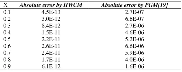
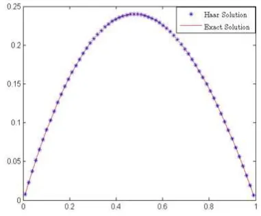
The comparison of exact and Haar solution for J =4 is shown in Figure 2. We have compared our results with Petrov - Galerkin method (PGM) [19] and are shown in Table 2.

Example 3: Consider the linear fifth order boundary value problem, which arises in the mathematical modeling of viscoelastic flows [17].

(5)

( )

x

(15 10 ),

(0,1),

y

x

−

y x

= −

e

+

x

∈

(33)

Subject to the boundary conditions:

(1) (1) ( 2)

(0)

0, (1)

0,

(0)

1,

(1)

,

(0)

0. y

=

y

=

y

=

y

= −

e y

=

(34)

Analytic solution is

y x

( )

=

(

x

−

x e

2

) .

x The comparison of exact and Haar solution with J =3 is represented in Figure 3. Table 3 cites the comparison numerically between HWCM and VIM, B-Spline, Homotopy perturbation method (HPM) , ADM [20].

Example 4: Consider the nonlinear equation

(5) 2

( )

x

( ),

(0,1),

y

x

=

e y x

−

where

x

∈

(35) subject to the boundary conditions:

(1) (2) (1)

(0)

1,

(0)

1,

(0)

1,

(1)

,

(1)

.

y

=

y

=

y

=

y

=

e y

=

e

(36)

The exact solution is

e

x

.

_{The nonlinear BVP (35) is converted into a sequence of linear BVPs with aid of}

quasilinearization technique [24]. For J =4 the comparison of exact and Haar solution for Ex. 4 is shown in Figure 4. In Table 4 errors obtained by the present method are compared with errors obtained by VIM, B-Splines, HPM and ADM [20].

Example 5: Consider the nonlinear BVP

(5) 5

5

48 ( ) 24

,

(0,1) ,

(1

)

y

x

e

x

−

+

=

∈

+

(37)

Subject to the boundary conditions:

(1) (2) (1)

1 (0)

0,

(0)

1,

(0)

1, (1)

log 2,

(1)

2 y

=

y

=

y

= −

y

=

y

=

. (38)

The exact solution is

log(1

+

x

).

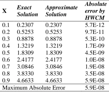
The comparison of exact and Haar solution for this example with J =3 is illustrated in Figure 5. The absolute errors obtained by HWCM are compared with PGM [19] is presented in Table 5.

Table - 1: Numerical Results for Ex.1.

X Exact

Solution

Approximate Solution

Absolute error by HWCM

(7)

Table - 2: Comparison of Numerical Results for Ex.2.

Table 3: Comparison of Numerical Results for Ex. 3.

X

Absolute error by VIM[20]

Absolute error by HPM[20]

Absolute error by ADM[20]

Absolute error by B-spline[20]

0.1 1.6E-11 3.0E-11 3.0E-11 3.0E-11 8.0E-03 0.2 1.0E-10 2.0E-10 2.0E-10 2.0E-10 1.2E-03 0.3 2.6E-10 4.0E-10 4.0E-10 4.0E-10 5.0E-03 0.4 4.7E-10 8.0E-10 8.0E-10 8.0E-10 3.0E-03 0.5 6.5E-10 1.2E-09 1.2E-09 1.2E-09 8.0E-03 0.6 7.4E-10 2.0E-09 2.0E-09 2.0E-09 6.0E-03 0.7 6.8E-10 2.2E-09 2.2E-09 2.2E-09 0.0E+0 0.8 4.6E-10 1.9E-09 1.9E-09 1.9E-09 9.0E-03 0.9 1.7E-10 1.4E-09 1.4E-09 1.4E-09 9.0E-03

Table-4: Comparison of Numerical Results for Ex. 4.

X Absolute error by

HWCM

Absolute error by VIM[20]

Absolute error by HPM[20]

Absolute error by ADM[20]

Absolute error by B-spline [20]

0.1 3.7E-13 1.0E-09 1.0E-09 1.0E-09 7.0E-04

0.2 2.4E-12 2.0E-09 2.0E-09 2.0E-09 7.2E-04

0.3 6.2E-12 1.0E-08 1.0E-08 1.0E-08 4.1E-04

0.4 1.1E-11 2.0E-08 2.0E-08 2.0E-08 4.6E-04

0.5 1.5E-11 3.1E-08 3.1E-08 3.1E-08 4.7E-04

0.6 1.6E-11 3.7E-08 3.7E-08 3.7E-08 4.8E-04

0.7 1.5E-11 4.1E-08 4.1E-08 4.1E-08 3.9E-04

0.8 9.6E-12 3.1E-08 3.1E-08 3.1E-08 3.1E-04

0.9 3.3E-12 1.4E-08 1.4E-08 1.4E-08 1.6E-04

Figure 1: Comparison exact and Haar Solution of Ex.1. Figure 1.1: Absolute errors by HWCM for J=3 of Ex. 1.

X Absolute error by HWCM Absolute error by PGM[19]

0.1 4.5E-13 2.7E-07

0.2 3.0E-12 6.6E-07

0.3 8.4E-12 2.7E-06

0.4 1.5E-11 4.6E-06

0.5 2.2E-11 5.2E-06

0.6 2.6E-11 6.6E-06

0.7 2.4E-11 5.9E-06

0.8 1.7E-11 4.0E-06

(8)

Figure 1.2: Absolute errors by VIM [23]. Figure 2: Comparison of exact and Haar Solution for Ex. 2.

Figure 3: Comparison of exact and Haar Solution for Ex. 3. Figure 4: Comparison of exact and Haar Solution for Ex. 4.

Table - 5: Comparison of numerical result for Ex. 5.

Table - 6: Comparison of maximum absolute errors of HWCM with various numerical methods. X

Absolute error by PGM[19]

0.1 2.7E-09 7.5E-08 0.2 1.9E-08 5.1E-07 0.3 5.5E-08 2.8E-06 0.4 1.1E-07 4.9E-06 0.5 1.7E-07 6.2E-06 0.6 2.3E-07 6.2E-06 0.7 2.4E-07 6.0E-06 0.8 2.0E-07 4.4E-06 0.9 9.1E-08 1.8E-06

Examples HWCM PGM

(Viswanadham et al.)[19]

VIM (Noor et al.)[20]

HPM (Noor et al.)[20]

ADM (Noor et al.)[20]

B-Spline (Viswanadham

et al.)[19]

Ex. 2. 2.6E-11 6.6E-06 - - - -

Ex. 3. 7.4E-10 - 2.2E-09 2.2E-09 2.2E-09 9.0E-03 Ex. 4. 1.6E-11 - 4.1E-08 4.1E-08 4.1E-08 7.2E-04

(9)

CONCLUSION

In this paper, we applied HWCM to solve fifth order IVP/BVPs. We established the error bound for the proposed method and concluded that Haar approximation is of order two. Nonlinear problems were solved with the aid of quasilinearization technique. Few test problems were taken to check the efficiency and applicability of the HWCM. It is evident from Figures 1 to 5 that approximate solution obtained by proposed method is comparable to the exact solution. We noticed from Tables 1 to 6 that HWCM has given better accurate results compared to other numerical methods viz. PGM, VIM, HPM, ADM and B-spline method. In the present method we achieved more precise results for less resolution values and it is a reliable technique for solving fifth order ODEs.

ACKNOWLEDGMENT

Authors are thankful to Prof. Ulo Lepik, University of Tartu, Estonia, for providing necessary and valuable comments/suggestions to improve this article. A. Padmanabha Reddy is grateful to Vision Group on Science and Technology, Govt. of Karnataka, India, for financial assistance under the scheme “Seed Money to Young Scientists for Research (SMYSR-FY-2015-16/GRD-497)”.

REFERENCES

1. C. G. Jaideva and K. C. Andrew, Fundametals of wavelets, John wiley and sons, New Jersey, USA, 2011, p. 34-146.

2. K. R. David and J. V. Patrick, Wavelet theory: an elementary approach with applications, A John Wiley, 2009, p. 85-172.

3. A. Haar, Zur theoric der orthogonalen Funktionsysteme, Math. Annal., 1910; 69, 331-371. 4. U. Lepik and H. Hein, Haar wavelets with applications, Springer, 2014, p. 7-42.

5. C. F. Chen and C. H. Hsiao, Haar wavelet method for solving lumped and distributed - parameter systems, IEEE Proc. Control Theory Appl., 1997; 144, 87-94.

6. C. F. Chen and C. H. Hsiao, Wavelet approach to optimizing dynamic systems, IEEE Proc. Control Theory. Appl., 1999; 146, 213-219.

7. U. Lepik, Haar wavelet method for solving higher order differential equations, Int. J. Math. Comput., 2008; 1, 84-94.

8. K. Harpreet, R. C. Mittal and M. Vinod, Haar wavelet quasilinearization approach for solving nonlinear boundary value problems, Amer. J. Comp. Math., 2011; 1, 176-182.

9. Siraj-ul-Islam, A. Imran and S. Bozidar, The numerical solution of second order BVPs by collocation method with the Haar Wavelets, Math. Comp. model., 2010; 52, 1577-1590.

10. Fazal-i-Haq and A. Arshed, Numerical solution of fourth order boundary value problems using Haar wavelets, Appl. Math. Sci., 2011; 63, 3131-3146.

11. Fazal-i-Haq, A. Arshed and H. Iltaf, Numerical solution of sixth-order boundary value problems by collocation method using Haar wavelets, Appl. Math. Sci., 2012; 43, 5729-5735.

12. Fazal-i-Haq, A. Imran and Siraj-ul-I., A Haar wavelet based numerical method for eight-order boundary problems, Int. J. Appl. Compt. Sci., 2010; 6, 25-30.

13. A. Padmanabha Reddy, S. H. Manjula, C. Sateesha and N. M. Bujurke, Haar wavelet approach for the solution of seventh order ordinary differential equations, Math. Mod. Eng. Prob., 2016;3, 52-58.

14. S. Saha Ray, On Haar wavelet operational matrix of general order and its application for the numerical solution of fractional Bagley Torvik equation, Appl. Math. Comp., 2012; 218, 5239-5248.

15. S. Saha Ray and A. Patra, Haar wavelet operational methods for the numerical solutions of fractional order nonlinear oscillatory Van der Pol system, Appl.Math.Comp., 2012; 220, 659-667.

16. G. Hariharan and K. Kannan, An overview of Haar wavelet method for solving differential and integral equations, Wl. Appl. Sci. J., 2013; 12, 01-14.

17. A. R. Davies, A. Karageorghis and T. N. Phillips, Spectral Galerkin methods for the primary two-point boundary value problem in modeling viscoelastic flows, Int. J. For Numerical Methods in Eng., 1998; 26, 647-662.

18. A. M. Wazwaz, The numerical solution of fifth order boundary value problems by the Decomposition method, J. Comp. Appl. Math., 2001; 136, 259-270.

19. K. N. S. Kasi Viswanadham and S. M. Reddy, Numerical Solution of Fifth Order Boundary Value Problems by Petrov-Galerkin Method with Quartic B-splines as basis functions and Sextic B-splines as weight functions, Int. J. Eng. Sci. Innov. Tech., 2015; 4, 2319-5967.

20. M. A. Noor, S. T. Mohyud-Din and A. Waheed, Variation of Parameters Method for Solving Fifth-Order Boundary Value Problems, Appl.Mat.Inf.Sci., 2008; 2, 135-141, 2008.

21. J. Majak, B. S. Shvartsman, M. Kirs, M. Pohlak and H. Herranen, Convergence theorem for the Haar wavelet based discretization method, Compos. Struct., 2015; 126, 227-232.

(10)

23. P. Mehdi Gholami, G. Behzad and G. Mohammad, He’s Variational Iteration Method for Solving Differential Equations of the Fifth Order,Gen. Math. Notes, 2010; 1, 153-158.

24. R. E. Bellman and R. E. Kabala, Quasilinearization and nonlinear boundary value problems, Amer. Elsevier, New York, 1965, p. 13-55.

Source of support: Science and Technology, Govt. of Karnataka, India, Conflict of interest: None Declared

[Copy right © 2016. This is an Open Access article distributed under the terms of the International Journal of Mathematical Archive (IJMA), which permits unrestricted use, distribution, and reproduction in any medium, provided the original work is properly cited.]