ORDER OF THE RUNGE-KUTTA METHOD AND EVOLUTION OF THE STABILITY REGION

DOI: 10.15826/umj.2019.2.006

ORDER OF THE RUNGE–KUTTA METHOD AND

EVOLUTION OF THE STABILITY REGION

Hippolyte Séka†, Kouassi Richard Assui††

Institut National Polytechnique Houphouët–Boigny, BP 1093 Yamoussoukro, Côte d’Ivoire †_{[email protected],} ††_{[email protected]}

Abstract: In this article, we demonstrate through specific examples that the evolution of the size of the absolute stability regions of Runge–Kutta methods for ordinary differential equation does not depend on the order of methods.

Keywords: Stability region, Runge–Kutta methods, Ordinary differential equations, Order of methods.

Introduction

Representations of the stability regions of Runge–Kutta methods are presented in several lit-eratures [1–8, 11, 13]. It has been found that the stability region varies according to the order of the method. However, it is not proven in the literature whether or not there is a relation between the evolution of the size of the region of stability and the order of the method. In this article, we demonstrate that the evolution of the size of the stability region does not depend on the order of the methods. For that we exhibit methods whose regions of stability grow according to the order. Sub-sequently, we give a counter-example where we introduce a new8 order method [12]. We compare the stability region of this new8order method with those of certain lower order methods. We show that the stability regions of lower order methods are larger than that of the new8 order method. The study will be done in accordance with the following plan: in Section 2 we describe some gen-eralities on the stability regions, in Section 3 we present some stability functions, in Section 4 we present the new8 order method and its stability regions, Section 5 we give a conclusion.

1. Generalities on the stability regions

Consider a general form of the first-order ODE given below:

y′ =f(x, y(x)), (1.1)

with the initial condition y(x0) = y0 for the interval x0 ≤ x ≤ xn. Here, x is the independent

variable, y is the dependent variable, nis the number of point values, and f is the function of the derivation. The goal is to determine the unknown functiony(x) whose derivative satisfies (1.1) and the corresponding initial values. In doing so, let us discretize the intervalx0≤x≤xn to be

x0, x1 =x0+h, x2=x0+ 2h, ..., xn=x0+nh,

1_{We would like to express our deepest appreciation and gratitude to Professor Sergey Khashin of Ivanovo}

where h is the fixed step size. With the initial condition y(x0) = y0, the unknown grid function

y1, y2, y3,· · · , yncan be calculated by using the Runge–Kutta method of the order 8 (RK8 method). The 8-th order method is thus obtained by the resolution of the200equations with 11 stages [12] on Maple.

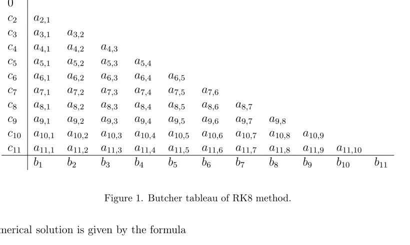
Lets consider the Butcher tableau of8 order and11 steps RK method (see Fig. 1):

0

c₂ a_2,1

c₃ a_3,1 a_3,2

c₄ a_4,1 a_4,2 a_4,3

c₅ a_5,1 a_5,2 a_5,3 a_5,4 c₆ a_6,1 a_6,2 a_6,3 a_6,4 a_6,5

c₇ a_7,1 a_7,2 a_7,3 a_7,4 a_7,5 a_7,6

c₈ a_8,1 a_8,2 a_8,3 a_8,4 a_8,5 a_8,6 a_8,7

c₉ a_9,1 a_9,2 a_9,3 a_9,4 a_9,5 a_9,6 a_9,7 a_9,8

c₁₀ a_10,1 a_10,2 a_10,3 a_10,4 a_10,5 a_10,6 a_10,7 a_10,8 a_10,9

c₁₁ a_11,1 a_11,2 a_11,3 a_11,4 a_11,5 a_11,6 a_11,7 a_11,8 a_11,9 a_11,10

b₁ b₂ b₃ b₄ b₅ b₆ b₇ b₈ b₉ b₁₀ b₁₁

Figure 1. Butcher tableau of RK8 method.

The numerical solution is given by the formula

yi+1 =yi+h

X11

s=1

bsks

, (1.2)

with

ks=f

xi+csh, yi+h s−1 X

j=1

as,jkj

, xi+1 =xi+h. (1.3)

The concept of absolute stability, in its simplest form, is based on the analysis of the behavior, according to the values of the step h, of the numerical solutions of the model equation [9–12]:

u′(t) =λu(t). (1.4)

Using (1.3) and (1.4), we obtain:

for s_≥1, ks=λ

yi+h s−1 X

j=1

as,jkj

;

which gives:

yi+1=ζ(hλ)yi.

Ifz=hλ, then the absolute stability region is the set

2. Presentation of some stability functions

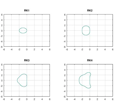
Consider the standard Runge-Kutta methods of orders1to 4. When (1.2) and (1.3) are applied to the model problem (1.4), the resulting equations are

RK1: yi+1 = (1 +z)yi;

RK2: yi+1 =

1 +z+z

2

2

yi;

RK3: yi+1=

1 +z+z

2

2 + z3

6

yi;

RK4: yi+1=

1 +z+z

2

2 + z3

6 + z4

24

yi.

The stability regions are shown at the next figure:

Figure 2. Evolution of the stability region according to the order.

3. Presentation of the new 8 _{order method and its stability regions}

The family of the8th order method is thus obtained by the resolution of the200 equations with 11 stages [12] on Maple. This method depends on free parameters b8 anda10,5 [12].

Some of related coefficients have fixed values, not depending on b8 and a10,5, these coefficients

are:

b1=

1

20; b2 = 0; b3 = 0; b4= 0; b5 = 0; b6 = 0; b9= 16

45; b10= 49

180; b11= 1 20;

c2 =

1

2; c3 = 1

2; c4=

7 +√21

14 ; c5 =

7 +√21

14 ; c6 = 1 2;

c7 =

7₋√21

14 ; c8=

7₋√21

14 ; c9 = 1

2; c10 =

7 +√21

14 ; c11= 1;

a2,1 =

1 2;

a3,1 =

1

4; a3,2= 1 4;

a4,1 =

1

7; a4,2=

−7₋3√21

98 ; a4,3 =

21 + 5√21 49 ;

a5,1 =

11 +√21

84 ; a5,2 = 0; a5,3 = 4√21

63 + 2

7; a5,4=

21₋√21 252 ;

a6,1=

5 +√21

48 ; a6,2 = 0; a6,3=

9 +√21

36 ; a6,4=

−231 + 14√21

360 ; a6,5=

63₋7√21 80 ;

a7,1=

10₋√21

42 ; a7,2= 0;

a9,1=

1

32; a9,2= 0;

a10,1 =

1

14; a10,2 = 0; a10,9 = 4√21

35 + 132 245;

a11,1 = 0; a11,2 = 0; a11,9 =

28₋28√21

45 ; a11,10=

49₋7√21 18 .

And the others are expressed in terms of b8 and a10,5:

b7 =−b8+

49 180;

a7,3=−(24/35)a10,5−136/105−(12/245)a10,5

√

21 + (656/2205)√21;

a7,4 = 7−(3/10)a10,5

√

21₋(71/45)√21 + (3/10)a10,5;

a7,5 =−(3/10)a10,5+ (3/10)a10,5

√

21₋43/6 + (169/105)√21;

a7,6=−(277/735)

√

21 + 181/105 + (12/245)a10,5

√

21 + (24/35)a10,5;

a8,1 =−

180b8

√

21₋49√21₋1800b8+ 343

7560b8

; a8,2 = 0;

a8,5=−

441a10,5

√

21₋3240a7,5b8−28

√

21 + 882a7,5−2205a10,5+ 147

3240b8

;

a8,6 =

72a10,5

√

21 + 1620a7,6b8−29

√

21₋441a7,6−252a10,5+ 119

1620b8

And also:

a8,3 =−

900b8

√

21 + 11340a7,2b8+ 11340a8,6b8−98

√

21₋3087a7,2−4860b8+ 686

11340b8

;

a8,7 =

49 1620b8

;

a8,4 =

(c2

8/2)−a8,2c2−a8,3c3−a8,5c5−a8,6c6−a8,7c7

c4

;

a9,3 = (1/8)a10,5

√

21₋(1/8)a10,5−(1/72)

√

21 + 1/72;

a9,4 =−49/288−(7/32)a10,5

√

21 + (7/288)√21 + (49/32)a10,5;

a9,5 = (7/32)a10,5

√

21₋(35/576)√21₋(49/32)a10,5+ 21/64;

a9,6=−(1/8)a10,5

√

21 + (1/8)a10,5+ (1/72)

√

21 + 5/36;

a9,7= 91/576 + (7/192)

√

21₋(585/1568)b8

√

21₋(405/224)b8;

a9,8 = (585/1568)b8

√

21 + (405/224)b8;

a10,3=−(6/49)a10,5

√

21₋(2/7)a10,5 + (2/147)

√

21 + 2/63;

a10,4 = 1/9−a10,5;

a10,6 = (2/7)a10,5−803/2205 + (6/49)a10,5

√

21₋(59/735)√21;

a10,7 = 1/9 + (1/42)

√

21 + (2295/686)b8+ (495/686)b8

√

21;

a10,8 =−(2295/686)b8 −(495/686)b8

√

21;

a11,3 = (2/3)a10,5

√

21₋(2/3)a10,5−(2/27)

√

21 + 2/27;

a11,4=−(7/6)a10,5

√

21 + (7/54)√21 + (49/6)a10,5−49/54;

a11,5 = (7/27)

√

21₋77/54₋(49/6)a10,5+ (7/6)a10,5

√

21;

a11,6 = (2/3)a10,5 −64/135−(2/3)a10,5

√

21 + (94/135)√21;

a11,7 = 7/18−(265/98)b8

√

21₋(215/14)b8;

a11,8= (265/98)b8

√

21 + (215/14)b8.

The numerical solution is given by the formula (1.2). The values ofksare given by the formula (1.3). We can notice that ifb8 = 49/180anda10,5 = 1/9, then we find the method of Cooper–Verner [1,12].

With the help of Maple, the stability function depends on a10,5 and is given by [12]:

ζ(z) = 1 +z+ 1 2z 2 +1 6z 3 + 1 24z 4 + 1 120z 5 + 1 720z 6 + 1 5040z 7 + 1 40320z 8 + − 797 50803200 + 1

25200a10,5+ 37 4233600

√

21a10,5−

499 152409600 √ 21 z9 + 1 470400+ 1 2083725 √

21₋ 31

940800a10,5− 61 8467200

√

21a10,5

z10

+

−_290304001 −_426746880013 √21 + 11

1612800a10,5+

353 237081600

√

21a10,5

For a10,5= 106 we find

ζ(z) = 1 +z+ 1 2z

2

+1 6z

3

+ 1 24z

4

+ 1 120z

5

+ 1 720z

6

+ 1 5040z

7

+ 1 40320z

8

+2015999203 50803200 z

9

−15499999₄₇₀₄₀₀ z10+ 197999999 29030400 z

11

+190285643 21772800

√

21z9₋60046871 8334900

√

21z10+6353999987 4267468800

√

21z11.

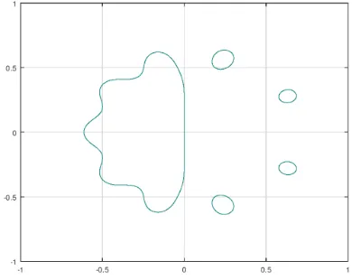
The stability region of the new RK8 method fora10,5 = 106 is given by Fig. 3.

Figure 3. Stability region of the new RK8 method fora10,5= 10 6

.

We can see that the stability region of the new method of order8 is smaller than2,3,4. There is a decrease in the values ofx and y.

For a10,5= 1012 the stability region is the following (see Fig. 4):

Figure 4. Stability region of the new RK8 method fora10,5= 10 12

.

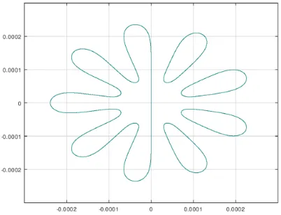
For a10,5= 9. . .9 | {z } 37times

the stability region is is shown at the next figure:

Figure 5. Stability region of the new RK8 method.

We find that the values of x andy have very strongly diminished and the region of stability is very small.

4. Conclusion

Presumably, by representing the domains of stability of methods of the order of 1, 2, 3, 4, one could assume that the higher the order, the greater the area of stability. However, a new 8 order method is discovered. The stability region of this8order method is smaller than that of the regions of orders2,3,4. We can therefore conclude that the evolution of the size of the stability regions of Runge-Kutta methods does not depend on the order of the method.

REFERENCES

1. Butcher J.-C.Numerical Methods for Ordinary Differential Equations.2nd ed. John Wiley & Sons Ltd., 2008. 175 p.DOI: 10.1002/9780470753767

2. Calvo M., Montijano J. I., Randez L. A new embedded pair of Runge–Kutta formulas of orders5and6. Comput. Math. Appl., 1990. Vol. 20, No. 1. P. 15–24.DOI: 10.1016/0898-1221(90)90064-Q

3. Cassity C. R. The complete solution of the fifth order Runge–Kutta equations.SIAM J. Numer. Anal., 1969. Vol. 6, No. 3. P. 432–436.DOI: 10.1137/0706038

4. Feagin T. A tenth-order Runge–Kutta method with error estimate. In: Proc. of the IAENG Conf. on Scientific Computing. Hong Kong, 2007. Accessible athttps://sce.uhcl.edu/feagin/courses/rk10.pdf

5. Feagin T.High-Order Explicit Runge-Kutta Methods. 2013. Accessible athttp://sce.uhcl.edu/rungekutta

6. Hairer E., Nørsett S. P., Wanner G. Solving Ordinary Differential Equations I. Nonstiff Prob-lems. Springer Ser. Comput. Math., vol. 8. Berlin, Heidelberg: Springer–Verlag, 1993. 528 p.

DOI: 10.1007/978-3-540-78862-1

7. Houben S. Stability Regions of Runge–Kutta Methods. Eindhoven University of Technology, 2002. Ac-cessible athttps://www.win.tue.nl/casa/meetings/seminar/previous/_abstract020220_files/talk.pd

8. Jackiewicz Z. General Linear Methods for Ordinary Differential Equations. John Wiley & Sons, Inc., 2009. 482 p.DOI: 10.1002/9780470522165

9. Khashin S. I.List of Some Known Runge-Kutta Methods Family.Preliminary version. 2013. Accessible athttp://math.ivanovo.ac.ru/dalgebra/Khashin/rk/sh_rk.html

11. Liu M. Z., Song M. H., Yang Z. W. Stability of Runge–Kutta methods in the numerical solution of equation u′_{(t) = au(t) +a0u([t]). J. Comput. Appl. Math., 2004. Vol. 166, No. 2. P. 361–370.} DOI: 10.1016/j.cam.2003.04.002

12. Seka H., Assui K. R. A New Eighth Order Runge-Kutta Family Method.J. Math. Res., 2019. Vol. 11, No. 2. P. 190–199.DOI: 10.5539/jmr.v11n2p190

13. Velagala S. R.Stability Analysis of the 4th order Runge–Kutta Method in Application to Colloidal Par-ticle Interactions. Master’s thesis. University of Illinois, Urbana-Champaign, USA, 2014. Accessible at