Vol 2, No 2 (2016)

(1)

Journal of Electrical Engineering,

Electronics, Control and Computer Science

JEEECCS, Volume 2, Issue 4, pages 13-20, 2016

FASharpSim: A Software Simulator for

Deterministic and Nondeterministic Finite

Automata

Georgiana-Mihaela NIȚU, Florin-Marian BÎRLEANU Department of Electronics, Computer Science and Electrical Engineering Faculty of Electronics, Communications and Computers, University of Pitești, Romania

[email protected], [email protected]

Abstract – FASharpSim is a didactic simulator for deterministic and nondeterministic finite automata meant to be used in the laboratory classes. It allows, before simulation, building these automata in an intuitive easy manner, by means of a simple friendly graphical interface. This application explains the concept of finite automaton by clearly simulating it. The paper describes the application development, the algorithms which provide its functionality (compilation, simulation), as well as some eloquent examples of designing and simulating some automata using FASharpSim. The purpose of the simulator is to clearly illustrate the notion of finite automaton and draw a sharp line between the two types of finite automata: deterministic and nondeterministic.

Keywords – deterministic finite automaton (DFA); nondeterministic finite automaton (NFA); ε-transitions; automata simulation.

I. INTRODUCTION

Finite automata have represented the first computing machines and have a crucial role in computer science and its evolution as we know it. Can we imagine our computers without finite automata? They are an essential model for hardware and software components and have numerous applications in nowadays computing activity: compiling a program, searching for text in documents, designing and validating digital circuits. The purpose of studying formal languages and automata is for the students and interested readers to get the feel of programming principles and how it works. Finite automata can be seen as minimalistic versions of programming languages, defined by a rigorous set of symbols and laws that dictate how to combine the symbols.

How is it possible to combine symbols in order to create valid words? The paper answers this question by introducing a compact simulation application for finite automata, FASharpSim, which depicts how these behave, how they can impose some restrictions and allow only a precise set of rules in order to obtain the required output (in this case the output being a yes (input word accepted) or a no (input word not accepted)). The simulator implements some concise algorithms for clarifying how an automaton processes input and gives a verdict about its category: accepted, or not accepted.

Over time, finite automata have been simulated using different methods, each of them bringing its valuable contribution to their understanding. In order to design and implement the simulator presented in this paper, a theoretical research has been undertaken by employing the text books [1], [2] and [3]. Afterwards, a study regarding the state of the art in simulating finite automata was performed. Such applications have been developed as desktop applications [4], [5], [6], as well as web applications [7], [8]. In [9] the author compares various simulators by presenting their relevant features. The novelty of our application is that it is dedicated exclusively to finite automata and clearly highlights the simulation steps (and also gives an answer to the user when simulation is complete).

The paper presents the key features of the simulator (Section II), how an automaton is seen by the simulator (Section III.A), how it gets verified after building it (Section III.B), what type of automaton we have built (Section III.C), how an input word finds its way to acceptance or not by using a step by step approach (Section III.D) and how an automaton gets saved to disk (Section III.E). Additionally, some examples of using the application are shown in Section IV and conclusions regarding the simulator and its usefulness are drawn in the last section.

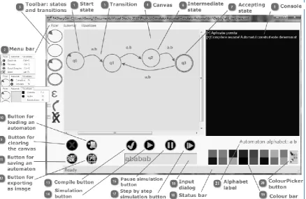
II. INTERFACEANDFUNCTIONALITIES FASharpSim is implemented in C# and allows editing and simulating Deterministic (DFAs) and Nondeterministic Finite Automata (NFAs), including ε-NFAs. Its friendly graphical user interface comes with a series of buttons and menus meant to provide the user with a pleasant experience in creating the desired automaton, by easily choosing the states and transitions from a tool bar and dropping them on a canvas.

(2)

Figure 1. FASharpSim graphical user interface.

III. ALGORITHMSANDIMPLEMENTATION All the functionalities described in the previous section are based on some key algorithms that build the behavior of our application. All the states of an automaton being edited are kept in a list. Also, a separate list keeps track of the transitions for a specific automaton. Both lists are used in the compilation and simulation algorithms, as described below. Besides algorithms, this section describes how states and transitions are represented in the computer memory and how transition curves are painted on the canvas.

A. Memory representation of the finite automaton The automata build with the simulator are transitions graphs, where nodes are states and arcs are labeled with input symbols, denoting transitions. Yet, what the computer "sees" is quite different from what the user builds: the simulator models the components of the automaton as UserControl objects that communicate with each other.Each state of the automaton is a UserControl, on which a circle is painted. It contains a TextBox component that allows the user to input a name for that particular state and a Label component for displaying that name. The main properties of a State are: Name, Index (in a list of states), and the boolean values Accepting and Start. Depending on the combination of the last two properties, we can build four types of states: start accepting state, start nonaccepting state, accepting and nonstarting state, and, lastly, non-accepting and nonstarting state. Likewise, the transitions are modeled as a UserControl containing a TextBox for inputting the input symbols that cause the transition to activate, as well as a Label for displaying those symbols. The most important members in the Transition class are IndexStartState and IndexStopState, i.e. the two indexes defining in fact

the transition. To complete the class, we also use StartName, StopName and GetSymbolList, which memorize the name of start and finish states, and, respectively, the transition symbols.

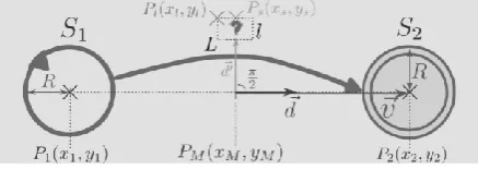
The UserControl is added on top a Bézier curve, representing the transition arc. This Bézier curve is drawn between the start and finish state that define the transition. The starting point of the curve is the centre of the start state. We recall that the states are circles painted on a UserControl. Let S1 be the start state and

S2 the finish state, P1(x1,y1) the centre of the start state

and P2(x2,y2)the centre of the finish state. The end

point for the curve, ( ), is the intersection of the vector with the circle that represents the stop state, as shown in Fig. 2.

Figure 2. Computing the coordinates for the end point of the Bézier curve that represents a transition.

The coordinates of P2(x2,y2) are computed using

(1).

(

√( ) ( ) ) ( )

(

√( ) ( ) ) ( ) ( )

(3)

FASharpSim: A Software Simulator for Deterministic and Nondeterministic Finite Automata 15

points are used to draw Béziers, we choose only one (multiple) point. Fig. 3 illustrates this point, PC(xC,yC),

positioned at a distance d = R from the center, PM of

the vector and rotated with 90 degrees.

Figure 3. The control point for the Bézier curve.

The control point coordinates are computed using (2), where xM and yM are the coordinates of the

midpoint of segment P1P2.

( )

√( ) ( )

( )

√( ) ( ) ( )

In order for the transition to be complete, it is needed to have the coordinates for the point where the label displaying the symbols is positioned (outside of the curve). Fig. 4 depicts the point ( ) representing the top-left coordinates of the Label component containing the symbols. To add symbols over the transition arc, we chose these to be painted at

a distance , fromthe vector , where R is the state radius, l is the Label height and L the Label width, as we can notice in Fig. 4.

Figure 4. The top-left point for the transition label.

The point where drawing begins is ( ) Its coordinates are computed relatively to the point ( ), whose coordinates, in turn, are described by (3).

( )

√( ) ( )

( )

√( ) ( )

( )

On the Ox axis, we choose , and for the Oy axis, we have two cases:

 If the start state is positioned to the left of the finish state, we coose .

 If the start state is positioned to the right of the finish state, we fix .

Equations (1), (2) and (3) are used in the Paint method associated to the PictureBox where the

automaton is drawn. We use the C# function DrawBezier to paint the curves.

B. Compiling an automaton

Before simulation, it is needed to know if the automaton that was built has some elements that make it a valid automaton: a single starting state, all states have a name and there is at least one accepting state. The function that implements the compilation of an automaton is illustrated by Algorithm 1.

Algorithm 1: Compiling an automaton.

1: function COMPILE 2: counterStart ← 0 3: okName ← true 4: if length(stateList) > 0

and length(transitionList) > 0 then 5: for each state s în stateList do 6: if s.Start = true then

7: counterStart ← counterStart + 1 8: if s.Name = ”” (empty string) then 9: okName ← false

10: if okName = false then

11: return "You did not name all the states!" 12: if counterStart ≠ 1 then

13: return "No start state or too many for the built automaton!”

14: if stateList.Any(st => st.Accepting) = false then 15: return "No accepting state for the automaton!" 16: return "Success!"

17: return "The automaton is not built!"

The application searches in the state list a state with the property start = true. When this particular state is found, a counter gets incremented. If counter≠ 1, an error is thrown: "No starting state or too many starting states for this automaton". Then, the algorithm looks for an empty string in the list named states. If at least one is found, the error "You did not name all the states" is raised. Similarly, states with the property accepting = true are searched. If none is found, the user gets the error "No accepting state for your automaton". Finally, if the automaton passes the three tests, it is considered correct and ready for simulation. Lines 4-9 check if there is only one start state and if all the states are named. Lines 10-13 return the corresponding errors. Line 14 is a Linq expression that searches in the state list at least one accepting state and if it finds one, it returns true. Hence, if the expression is false, line 15 gets executed. Line 16 signals a correct compilation. If neither states nor transitions are built by the user (i.e., the stateList or the transitionList is empty), the compilation fails with the error in line 17.

C. Deterministic or not?

(4)

illustrating the idea of the algorithm is shown in Fig. 5.

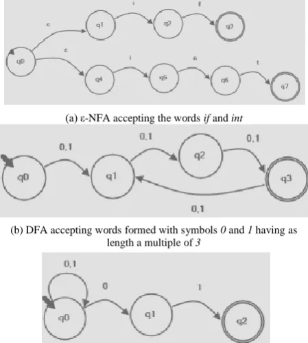
In Fig. 5a, the alphabet of the ε-NFA is Σ = {ε, i, n, t, f}. Because (q0, q1) and (q0, q4) are ε-transitions, the algorithm will tell the user that the automaton is nondeterministic. Following Fig. 5b, Σ = {0, 1}. For each state in the automaton, q0, q1, q2, q3, the symbols from the transition that starts with that state are {0, 1}. We notice that they form the same set as Σ. Therefore, the automaton is deterministic. Lastly, in Fig. 5c, the alphabet is Σ = {0, 1}. If we analyze state q0 and the transitions that leave from it, (q0, q0) and (q0, q1), we see that the list of symbols for the state q0 is {0,0,1}, which does not equal Σ. Also, we can observe that starting from q0, the automaton reaches two states simultaneously by following the symbol 0: q0 and q1. This leads to a nondeterministic automaton.

(a) ε-NFA accepting the words if and int

(b) DFA accepting words formed with symbols 0 and 1 having as length a multiple of 3

(c) NFA accepting words formed with 0 and 1 and ending in 01.

Figure 5. Examples of automata for illustrating the idea of the determinism checking algorithm.

D. Method for simulating an automaton

Simulating an automaton means starting from the start state and analyzing one by one the input symbols until the input word ends, in order to obtain an answer regarding whether the word is accepted or not. If this path ends in an accepting state, the word belongs to the language described by the automaton. Otherwise, it gets rejected. The simulation algorithm considers the DFAs as a particular case of NFAs, where only one next state is allowed for any state for a certain input symbol. The algorithm uses two boolean arrays to mark the current state and the next state. The main steps for the simulation algorithm are:

a) Find the starting state in the list of states and get its index, start. Mark the start state as current: here[start] ← true;

b) Compute the ε-closure for the start state – find the transition leaving the start state and,

if they contain ε symbol, mark the end state as current;

c) Compute the ε-closure for each state s from the state list: here[indexOf(s)] ← true; d) If we are in a certain state and the input

symbol equals the one on a transition from that state, mark the next state: willBeHere[indexOf(s)] ← true;

e) If the input string has ended and the automaton reached an accepting state, the string is accepted.

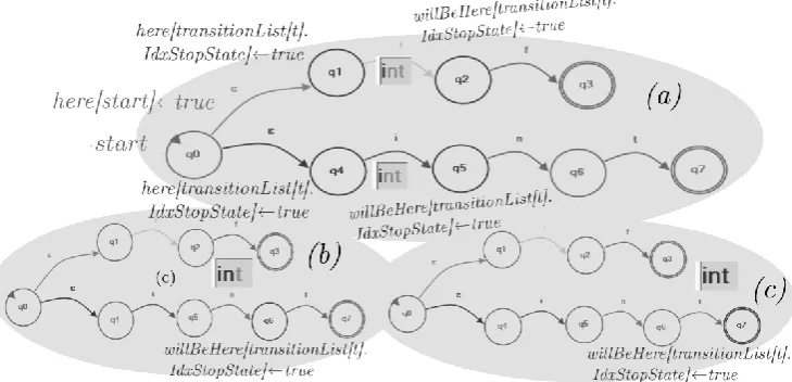
An example of how the algorithm works is provided in Fig. 6. Any finite automaton can be simulated using the method presented in this section. The automaton in Fig. 6 accepts the words if and int. Simulation takes place in steps (a), (b) and (c). At step (a), input symbol i causes the automaton to take ε-transitions (q0,q1) and (q0,q4). The ε-closure is computed for the start state. The current state is, therefore, {q0, q1, q4}. The algorithm searches the transition list and finds two transitions corresponding to input i: (q1, q2) and (q4, q5). The automaton takes these two transitions and the next state is {q2, q5}. After each step, the next state becomes the current state. At step (b), symbol n appears on the input, the algorithm finds the corresponding transition, (q5, q6), and the automaton reaches state q6. Step (c): the automaton takes the transition corresponding to t, (q6, q7), and reaches state q7. The input int ends and the simulator checks if the automaton remained in an accepting state. State q7 is indeed accepting and the application tells the user that the input string int is accepted by the automaton.

E. Saving an automaton to the disk

The simulator saves a built automaton as an XML file, which contains the set of states, stored in the node <states> and the transition set as <transitions>. For each state, a node <state> is build and the following information is saved for it: name, index, if it is a start state or not, if it is accepting or not, the screen location and the color. The <state> node is parent to all the nodes mentioned. For instance, the <state> node for an accepting state, nonstarting, blue, with top-left coordinate at point P(494,222) looks as in Listing 1.

Similarly to states, the transitions are saved in the same manner: each has a corresponding node contained in one <transitions> node. For each transition, the simulator saves: start state index, stop state index, the set of symbols and the color.

Listing 1: The XML format for a state.

<state> <name>q3</name> <idx>1</idx> <start>false</start> <accepting>true</accepting> <location>{X=494,Y=222}</location> <color>−12490271</color> </state>

Listing 2: The XML format for a transition.

(5)

A <transition> node for a transition starting from state with index 1 and ending in state with index 3, blue, activating on inputs a and b is shown in Listing 2.For building the XML file, we used the Linq library and XDocument and XElement objects.

IV. TESTINGANDRESULTS

In order to fully grasp the insights of how finite automata work and how the application tackles them, this section shows the results of a series of tests on some automata by using Algorithm 1 and the simulation method described in Section III.D on two examples designed with the simulator.

Example 1. Let there be a deterministic automaton which accepts the words formed with a and bso that no input symbol appears consecutively more than two times. It was designed with FASharpSim and its image is shown in Fig. 7. The simulation steps for an accepted input word are shown in Fig. 8.

Figure 6.The idea of the simulation algorithm.

Figure 7. DFA accepting words formed with a and b having no more than two identical adjacent symbols.

Example 2. Let there be the following ε-NFA, which accepts the language of words formed with a and bso that they have at least an a on the last four positions. If a string has less than 4 characters, it must contain at least an a on the last four positions in order to be accepted.

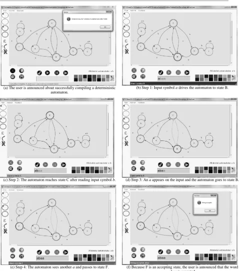
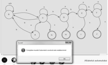
Fig. 9 depicts the automaton that accepts the language specified in this second example. We simulate this automaton for an input word that does not correspond to its language, as it can be noticed in Fig. 10. Simulation steps are as follows: after the user compiles the automaton (Fig. 10a), the input symbol b is processed and the automaton reaches state B (Fig. 10b). At Fig. 10c, an a causes the automaton to remain in B and also pass to C. In Fig. 10d, at the next step, the algorithm computes the ε-closure for state C and the automaton reaches state G, following the

(6)

Figure 8. Simulating the automaton from Example 1, Fig. 7, for the accepted input word abaa.

Figure 9. ε-NFA accepting words formed with a and b having at least an a on last 4 positions. (a) The user is announced about successfully compiling a deterministic

automaton.

(b) Step 1: Input symbol a drives the automaton to state B.

(c) Step 2: The automaton reaches state C after reading input symbol b. (d) Step 3: An a appears on the input and the automaton goes to state B.

(7)

(a) The user is announced about successfully compiling a nondeterministic automaton.

(b) Step 1: The automaton reads input b and passes to state B.

(c) Step 2: The automaton reaches states C and B after processing symbol a.

(d) Step 3: A b appears on the input and the automaton goes to states D, B and G.

(e) Step 4: The automaton sees another b and passes to states E, B and H.

(f) Step 5: Another b leads the automaton to states F, B and I.

(g) Step 6: The automaton sees the last symbol, b, and passes to states J and B.

(h) The automaton leaves state J. The user is announced the string babbbb is not accepted.

(8)

CONCLUSION

We introduced in this paper a simulator for deterministic and nondeterministic finite automata focused on their functionality in order to outline their manner of operating and to simplify their design in the laboratory classes, the emphasis being laid on their understanding. Likewise, we depicted the algorithms on which our application is based and discussed details about implementation. The application provides the user with an answer at the end of the simulation, after the entire input symbols were consumed. This simulator can be seen as a light tool to verify correctness of the built automata, to test and closely observe the evolution of states with respect to the input. During simulation, the current transition is highlighted in a random color and the current state becomes red in order for the user to clearly notice the correspondence between the automaton answer and the current input symbol. Pointing out this correspondence was the main purpose of the application.

The simulator can be extended by adding new functionalities: a mechanism for minimizing DFAs, the possibility of conversion from NFA to DFA and from ε-NFA to regular expressions and the other way round. If we consider the interface, this could be enhanced by adding a stop button for the continuous simulation (practically, that would reset the

simulation) and a button for stepping backwards into the simulation. Also, good features would be: to move more states at a time on the canvas and to be able to add symbols on the transitions in this manner: a..z (i.e., a range of symbols, in this case all the English letters) when it is necessary.

REFERENCES

[1] J. E. Hopcroft, R. Motwani, and J. D. Ullman, Introduction to Automata Theory, Languages, and Computation, Second Edition. Addison-Wesley, 2001.

[2] P. Linz, An Introduction to Formal Languages and Automata, Third Edition. Jones and Bartlett Publishers, 2001.

[3] G. V. Orman, Limbaje Formale.Bucureşti: Editura tehnică, 1982.

[4] T. M. White, T. P. Way, jFAST: A Java Finite Automata Simulation, Applied Computing Technology Laboratory, Department of Computing Sciences, Villanova University, In Thirty-seventh SIGCSE Technical Symposium on Computer Science Education (2006), 384–388, vol. 38.

[5] S. H. Rodger, T. W. Finley, JFLAP: An Interactive Formal Languages and Automata Package. Jones and Bartlett Publishers, 2006.

[6] C. Burch, "Automaton Simulator" (version 1.2), http://www.cburch.com/proj/autosim/, 2008.

[7] I. Zuzak, and V. Jankovic, "FSM simulation", http://ivanzuzak.info/noam/webapps/fsm_simulator/, 2015. [8] C. Burch, "Finite automaton simulation",

http://www.cs.cmu.edu/~cburch/survey/dfa/.