Predefined pattern detection in large time series

(1)

Contents lists available atScienceDirect

Information Sciences

journal homepage:www.elsevier.com/locate/ins

Predeﬁned pattern detection in large time series

Shengfa Miao

a,b,∗

_{, Ugo Vespier}

b

_{, Ricardo Cachucho}

b

_{, Marvin Meeng}

b

_,

Arno Knobbe

b

a_{Lanzhou University, Lanzhou, China} b_{Liacs, Leiden University, The Netherlands}

a r t i c l e

i n f o

Article history: Received 1 April 2014 Revised 5 April 2015 Accepted 11 April 2015 Available online 17 April 2015

Keywords: Pattern detection Landmark Trust region MDL

Predeﬁned pattern Time series representation

a b s t r a c t

Predefined pattern detection from time series is an interesting and challenging task. In order to reduce its computational cost and increase effectiveness, a number of time series represen-tation methods and similarity measures have been proposed. Most of the existing methods focus on full sequence matching, that is, sequences with clearly defined beginnings and end-ings, where all data points contribute to the match. These methods, however, do not account for temporal and magnitude deformations in the data and result to be ineffective on several real-world scenarios where noise and external phenomena introduce diversity in the class of patterns to be matched. In this paper, we present a novel pattern detection method, which is based on the notions of templates, landmarks, constraints and trust regions. We employ the Minimum Description Length (MDL) principle for time series preprocessing step, which helps to preserve all the prominent features and prevents the template from overfitting. Tem-plates are provided by common users or domain experts, and represent interesting patterns we want to detect from time series. Instead of utilising templates to match all the potential subsequences in the time series, we translate the time series and templates into landmark sequences, and detect patterns from landmark sequence of the time series. Through defin-ing constraints within the template landmark sequence, we effectively extract all the mark subsequences from the time series landmark sequence, and obtain a number of land-mark segments (time series subsequences or instances). We model each landland-mark segment through scaling the template in both temporal and magnitude dimensions. To suppress the influence of noise, we introduce the concept oftrust region, which not only helps to achieve an improved instance model, but also helps to catch the accurate boundaries of instances of the given template. Based on the similarities derived from instance models, we introduce the probability density function to calculate a similarity threshold. The threshold can be used to judge if a landmark segment is a true instance of the given template or not. To evaluate the effectiveness and efficiency of the proposed method, we apply it to two real-world datasets. The results show that our method is capable of detecting patterns of temporal and magnitude deformations with competitive performance.

∗ _{Corresponding author at: Liacs, Leiden University, The Netherlands.}

E-mail addresses: [email protected] (S. Miao), [email protected] (U. Vespier), [email protected] (R. Cachucho), [email protected](M. Meeng),[email protected](A. Knobbe).

(2)

1. Introduction

This paper focuses on the problem of detecting instances of predeﬁned patterns from time series[15,56]. While most pattern detection algorithms in time series deal with discovering previously unknown, frequently recurring regularities in the data, here we assume that one or more example sequences (thetemplates) are provided by a domain expert, and instances of these need to be identiﬁed in the actual data. During this detection, one needs to allow for a certain degree of difference between the template and the instances, for example because the instance is somewhat longer or shorter in duration, the magnitude of the signal is different, or parts of the signal are either stretched or compressed in time (so-called warps).

Li Wei et al.[56]mention a number of use-cases that motivate the predefined pattern detection problem. For example, in ECG monitoring, a cardiologist may observe some interesting pattern that he or she wants to annotate, and flag any future occurrences, to be investigated by the cardiologist or fellow experts. Alternatively, in insect pest control, one would like to observe specific cases of harmful insects, as identified by specific patterns of audio signal (wing beats). In our application to infrastructure monitoring, the predefined pattern detection problem is relevant for specifying and detecting known disturbances in the data, that can then be removed from the signal, or accounted for in subsequent modelling steps. For example, when monitoring the structural health of a bridge, the measured signal is dominated by recurring and understandable peaks due to vehicles crossing the bridge and traffic jams. One can imagine an expert providing a template for each of these phenomena, after which all instances should be identified, regardless of the speed and weight of the vehicles (influencing the width and height of the hump in the signal), or the duration of the traffic jam.

When matching a predefined phenomenon (a template[40,41,48]) with the time series under investigation, it is not always required to involve every individual measurement in the selected interval and in the template. In fact, when a certain level of fuzzy matching is required, it makes sense to somehow simplify the signal, or extract some key features that are characteristic for the sequence in question. This condensed representation can then be used to compare the time series with the template, both effectively (the matching is only based on the characteristic aspects) and efficiently (no computation is wasted on insignif-icant details). Specifically when large time series with high sampling rates are concerned, and the matching is nontrivial due to warps, efficient representation methods can be helpful. A considerable number of such methods have been proposed in the past, including Symbolic Aggregate approXimation (SAX)[29], bit-level approximation[7], and Piecewise Aggregate Approximation (PAA)[25]. 1 _{In this paper specifically, we focus on the representation of time series by means of}_landmarks_[43]_{(also referred} to as key-points[8], break-points[47]and change-points[37]), which can be thought of as those points in the time series that are obviously remarkable (peaks, valleys, inflection points, …). Rather than matching every detail of the data and the template, only the landmarks will be matched, and subsequent landmarks will be checked for their relationship to one another.

We match the given template to the actual data in three steps. The ﬁrst step involves transforming the time series into a sequence of landmarks, which preserves all the prominent features. The second step is landmark subsequence selection, which is based on constraints over the landmarks occurring in the templates. The third step is instance model construction, which introduces atrust regionto model the time series segments corresponding to the selected landmark subsequence. Unlike most of the representation and similarity methods, which are designed mainly for full sequence matching[15], our proposed approach is capable of processing both full sequence and subsequence matching of various length, while being less sensitive to noise, and being able to handle deformations in both magnitude and temporal dimensions.

One of the challenges when extracting landmarks from actual data is the noise and high-frequency vibrations that are in-cluded. An obvious step to get rid of such distractions and to produce a set of meaningful landmarks is to convolve the signal with a smoothing kernel. The question now becomes what level of smoothing is appropriate for the template in question. Too much smoothing may cause one to miss characteristic landmarks in the data, and too little smoothing will cause an abundance of landmarks at every little disturbance in the data. We propose an MDL-based solution to this challenge, that picks the correct smoothing level. Minimum Description Length (MDL)[20,49,51]is an information-theoretic model-selection framework that selects the best model according to its ability tocompressthe given data.

The contributions of this paper are summarised as follows:

• It provides a general deﬁnition of a template for time series.

• It proposes the use of landmarks: a triple involving temporal, magnitude and type information.

• It takes the relationship between landmarks within a landmark sequence as constraints for landmark subsequence selection. • It introduces the concept of a trust region from the image processing domain[32]to time series to build a reliable instance

model.

• It employs MDL[20,49,51]for selection of the right smoothing level for landmark extraction.

The rest of this paper is organised as follows. Section2gives the definitions of template and landmark, and specifies the task of predefined pattern detection. Section3introduces the concept of landmark constraints. The question of choosing the right smoothing level through MDL is discussed in Section4. In Section5, instance models are used to fit the template to

(3)

candidate instances in the data. Section6evaluates the proposed method by applying it to two datasets. Section7gives a litera-ture review of related work, followed by a conclusion in Section8.

2. Preliminaries

In this section, we will review and deﬁne some notation used throughout this paper. We begin by reviewing the concept of time series and subsequences, then give precise deﬁnitions of templates and landmarks.

Deﬁnition 1. Atime series T is an ordered sequence of n real values:

T=

(

t1,t2,. . .,tn

)

, ti∈R

h1,h2,. . .,hk

)

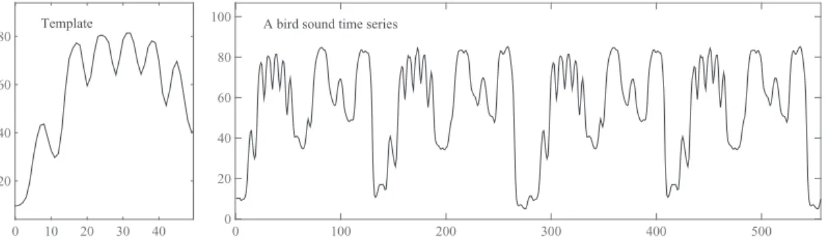
, hi∈R

A example is given in theFig. 1. The template in the left picture ofFig. 1stands for a piece of bird song[45], which helps us ﬁnd recurring subsequences from the time series in the right picture ofFig. 1.

2.1. Landmark extraction

Although we expect the user to specify the predefined pattern in terms of a template, we will not be matching the template directly to subsequences of the given time series. Rather, we intend to extract importantlandmarks[43]from both the template and the time series, and use these to match more efficiently and effectively. A landmark is defined as follows:

Deﬁnition 4. Given a time seriesT₌

(

t1,t2,. . .,tn

)

, alandmarkis a remarkable point inT, speciﬁed by a triplel:

l=

(

id,mt,type

)

, id∈N,mt∈R

whereidis the index of the landmark in the time seriesT,mt is the magnitude of the landmark,typeis the peak type indicator, which can be a local extreme, an inﬂection point or some other notable characteristic of the time series at this point.

We need to employ alandmark extractionmethod to produce a sequenceL of landmarks from a given time series. Such a method, generally identiﬁed as a functionE, can be applied to obtain a sequence of remarkable points from a given time series, but equally, it can be used to produce such points from a template, as that is essentially a time series also.

Landmark extraction methods are typically application dependent. In general, local extrema of the time series are good land-mark candidates. They are found by considering the zero-crossings of the first derivative of the series. These zero-crossings (roots) correspond to the extrema in the time series, which we assume to be of interest. Theinflection pointsderived from the extrema in the first derivative time series can also be considered as landmark candidates. Such landmarks can be found by looking at the zero-crossings of the second derivative. For a discrete time series, it may happen that a root is between two successive points of the time series. In this situation, we refer to the point close to zero as the zero-crossing point.

A landmark sequence preserves the main features of the time series, but signiﬁcantly reduces its representation size. As shown inFig. 2, the subsequence of length 900 can be compressed to a landmark sequence of only 16 elements

(

l1,l2,. . .,l16

)

.

Given a landmark subsequenceLa=

(

l1,l2,. . .,lm

)

and a time seriesT, there is a subsequence in the time series corresponding to it. The subsequence is referred as alandmark segmentLS. The index of the ﬁrst point ofLS is derived from the index ofl1, and that of the end point ofLS is derived from the index oflm.

2.2. Predeﬁned pattern detection

(4)

0 10 20 30 40 20

40 60 80

0 100 200 300 400 500

0 20 40 60 80

100 _{A bird sound time series}

Template

Fig. 1.An example of a template and time series. The curve in the left picture is a given template; the right picture illustrates a time series, in which subsequences similar to the template are expected.

1700 1800 1900 2000 2100 2200 2300 2400 2500

-5 0 5 10

0 50 100 150 200

0 1 2 3 4 5 A B C l₃ l 1 l

2 l4

l 5 l 6 l 7 l₈ l 9 l 10 l 11 l 12 l 13 l 14 l₁₅ l₁₆ Template

The first derivative

Part of a time series

Fig. 2. The landmark sequence. The curve in the left picture is a template, marked with landmarks A, B and C; the black curve in the right picture is part of a time series, and the grey curve is its ﬁrst derivative transform; the landmarksl1,l2,. . .,l16are derived from the ﬁrst derivative method.

Deﬁnition 5. The task ofPredeﬁned Pattern Detectiontakes as input a time seriesT of lengthn, a templateH of lengthkand a landmark extraction methodE_σ , and produces a sequences of matchesM=

(

LS1,LS2,. . .,LSp

)

, where eachLSi is a matched landmark segment inT,0≤p≤nis number of the matched subsequences.

There are two terms in the deﬁnition that should be addressed in more detail, one of which is the landmark extraction method

E_σ. As mentioned, we are not matching the template to the time series directly, but rather extracting landmarks from both ﬁrst, usingE_σ. An important parameter inEis

σ

, which helps to extract landmarks from the time series. If landmarks are deﬁned as zero-crossings,

σ

determines the level of smoothing applied to the raw time series. By smoothing, we prevent noise from playing a role in determining what constitutes a landmark. Of course, the level of noise (as opposed to the actual signal) depends on the application, so for the moment we assume this as simply a parameter of the task.

Another term is the sequence of matchesM. A time series subsequence is considered a matching landmark segmentLSi, if it can be conditionally transformed from the given templateH, with acceptable similarity. Given a template, we want to detect its instances from the time seriesT. These instances are allowed to have a certain level of temporal or amplitude variation, but they should preserve all the prominent features of the template. The matches can be obtained with landmark constraints (in Section 3) and instance models (in Section5).

In general, we assume the domain expert to provide additional information on the template in the form of constraints on the duration of the pattern as well as its magnitude. These will be expressed as lower and upper bounds on the duration of the pattern, as well as lower and upper bounds on the difference between the highest peak and the lowest valley. Clearly, without providing such constraints, one could stretch or compress the template to, say, a single data point or zero magnitude, losing all descriptive information in the template, while still matching many segments of the data.

3. Landmark constraints

In theory, for a given template landmark sequence of lengthk and a time series landmark sequence of lengthn, there aren₋k₊1 candidate landmark subsequences. Compared with the subsequence candidates from the original time series, the number has already been reduced a lot. However, the candidate number can be further reduced by employing landmark constraints of template landmark sequence. In this section, we introduce landmark constraints to break the time series landmark sequence into a number of meaningful landmark subsequences.

(5)

For example, given the template of length 200 (marked with landmarksA,BandC), shown as the left picture ofFig. 2, we are required to extract all the instances, whose lengths are between 80 and 350, from the time series, shown as the right picture of Fig. 2. The constraint set could be speciﬁed as follows:

• The length of landmark subsequences should be 3.

• The ﬁrst and last landmark of each subsequence should be valley points. • The second landmark of each subsequence should be a peak point.

• The index difference between the last landmark and the ﬁrst landmark should be between 80 and 350.

The first three constraints are used to preserve the main features of the template, and the forth constraint is used to meet conditions provided by users or domain experts. With these constraints, the number of landmark subsequence candi-dates can be significantly reduced (for the given subsequence, the number is reduced from 14 to 7, by 50%). Each landmark subsequence corresponds to a landmark segment, so the number of landmark segments is also significantly reduced. We will introduce instance model to fit the selected landmark segments in the Section5, which helps to further filter out false instances.

4. Determining the smoothing level

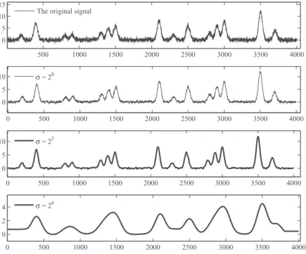
In practice, a time series, collected from a speciﬁc ﬁeld, is composed of both meaningful events and noise. Sometimes, the meaningful events are even buried by the noise. In order to make landmark extraction methods work effectively, we need to smooth the time series. When smoothing a time series, there is clearly a trade-off at play. Smoothing too little will produce a time series that shows too many landmarks, and smoothing too much will remove most of local features, such that impor-tant landmarks may be overlooked (seeFig. 3). In this section, we tackle the challenge of setting an appropriate value for the smoothing scale

σ

inE_σ.

IM

)

is the length, in bits, of the description of the time series when encoded with the help of the instance modelIM, that is the residual information not represented byIM.

A good, detailed model that catches most features of the target dataset leads to a low cost ofL

(

T

|

IM

)

, but a good model also means a higher cost compared with a simple model. Therefore, a trade-off between model ﬁt and its complexity is guaranteed by considering the size of the encoding. This property prevents the MDL method from overﬁtting.

When we calculateL

(

IM

)

andL

(

T

|

IM

)

, we assume that the valuesti of the input time seriesT have been quantised to a ﬁnite number of symbols by employing the function deﬁned below:

(6)

500 1000 1500 2000 2500 3000 3500 4000 0

5 10 15

0 500 1000 1500 2000 2500 3000 3500 4000

0 5 10

0 500 1000 1500 2000 2500 3000 3500 4000

0 5 10

0 500 1000 1500 2000 2500 3000 3500 4000

0 2

4 σ = 26

σ = 22

σ = 20

The original signal

Fig. 3. Various scales of smoothing. The ﬁrst picture shows the original time series without any preprocessing; the second picture shows the smoothed time series with a scale ofσ=20_{, which still contains considerable noise; the third picture shows the smoothed time series with a scale of}_σ₌₂2_{, which suppresses}

the noise and preserves the interesting patterns; the fourth pictures shows the smoothed time series with a scale ofσ=26_{, which suppresses both the noise}

and the interesting features.

)

indicates the fraction of points in the time series which has valuev.

Given the deﬁnition of entropy, we can deﬁne the description length of the second part of MDL as follows:

Deﬁnition 7. Given a time seriesT of lengthn, thedescription lengthofL

(

T

|

IM

)

(in bits) is given by

L

(

T

|

IM

)

=n·Entropy

(

T

|

IM

)

4.2. Smoothing scale selection

(

IM

)

=2r·log₂n

(7)

L

(

T

|

IM

)

=n·Entropy

T−

i=r

i=1

Tsi

whereTsi is theith landmark segment in the smoothed time seriesTs.

For a given template and a set of smoothing scale candidates, we assume that the optimal smoothing scale is the one that leads to the minimal MDL score.

5. Instance models

Given a landmark segmentLS of lengthmand a templateH of lengthk, we can simply modelLS by scalingH in both temporal and magnitude dimensions. The temporal scale operationX−scale results in a new sequenceIMX , whose length is the same as that of the landmark segment.

IMX =X−scale

(

H,m,k

)

, k,m∈N

X−ratio=m/k

IfX−ratio>1 , theX−scale is an up-sampling operation, and ifX−ratio<1 , theX−scale is a down-sampling operation, otherwise, theIMX is the same as the templateH.

IMXY

)

.

Based on the transformations mentioned above, we can deﬁne the instance model as:

Deﬁnition 8. Given a landmark segmentLSof lengthm, and a templateH of lengthk, theinstance modelIM ofLS is a sequence derived from transformations of the templateH:

IM=Trans f

(

LS,H

)

whereTrans f are the transformations deﬁned above (X−scale andY−scale).

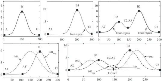
The advantage of obtaining instance models with the transformations mentioned above, is that they are straightforward and work well with regular landmark segments. However, when warps or distortions exist in landmark segments, the transformations will become insufficient. To illustrate the problem, we present a template, shown as the curve in the top left picture ofFig. 4, and use it to model three landmark segments: the curve in the top middle picture ofFig. 4is the first landmark segments, which is a single peak; the curve in the top right picture ofFig. 4is the second and the third landmark segments, which is composed of two overlapping peaks. The dotted curve IM1 in the bottom left picture ofFig. 4is an instance model obtained by simply transforming the given template. The instance model indicates that the left boundary of the first landmark segment is incorrect, which is caused by the false landmark A1. The dotted curves IM2 and IM3 in the bottom right picture ofFig. 4are two instances models, which are also obtained by simply transforming the given template. The boundaries of the landmark segments are correctly caught, but their instance models are still incorrect. This is caused by the complex (overlapping) nature of the time series. To overcome all these limitations, we introduce the notion of trust region.

5.1. Trust region

By assuming part of the landmarks within a landmark subsequence are reliable, in its landmark segment, we can define the corresponding segment between these landmarks as the trust region, shown as the thick regions in the top middle and right pictures ofFig. 4. Trust region is a concept borrowed from the field of image processing. We introduce the concept into time series (or to be more precise, into the instance model), and define it as:

Deﬁnition 9. Given a landmark segmentLS of lengthm, and its landmark sequenceL=

(

l1,l2,. . .,lm

)

of lengthm, if the segment between landmarksli andlj (1≤i< j≤m) is inﬂuenced less by noise, then thetrust regionofLS is deﬁned as:

LStrust=

(

tc1,. . .,td1

)

, 1≤c1<d1≤m

(8)

100 200 300 0

5 10

0 50 100 150 200 250 300 0 2 4 6 8 10

50 100 150 200 250 300 0

5 10

0 50 100 150 200 250

0 5 10

0 100 200

0 1 2 3 4 5 Trust-region C1 A1 A1' C1 A1 B C A B1 B1 Trust-region Trust-region A2 B2 C2/A3 B3 C3 A2 IM2 B2 C2/A3 B3 IM3 C3 IM3_imp IM2 imp C2'/A3' IM1 IM1_imp

Fig. 4.The instance model. The curve in the top left picture is the given template, which is marked with landmarks A, B and C; the segment between the landmarks B1 and C1 in the top middle picture is chosen as the trust region; in the top right picture, the segment between the landmarks A2 and B2 is the trust region of the ﬁrst landmark segment, and that between the landmarks B3 and C3 is the trust region of the second landmark segment; the dotted curves in the bottom left and right pictures are instance models simply obtained with transformations of the given template; the dashed curves in the bottom left and right pictures are improved instance models based on the trust regions in the top middle and right pictures.

Algorithm 1. The instance model.

Require: a templateH, and its landmark sequenceLHof lengthk, a landmark segmentLS, and its landmark sequenceLS of lengthk. Ensure: an improved instance modelIMimpand an updated landmark segmentLSup

LStrust=LS,Htrust=H

[IMimp,LSup]=Model(LS,LStrust,H,Htrust) simmax=Similarity(IMimp,LSup) forlen=2 tokdo

forindex=1 tok−len+1do

[LHtrust,LStrust]=LandmarkRegion(LH,LS,index,len) [Htrust,LStrust]=SegmentRegion(LS,H,LHtrust,LStrust,index,len) [IMtemp,LStemp]=Model(LS,LStrust,H,Htrust)

sim=Similarity(IMtemp,LStemp) ifsim>simmax then

simmax=sim

IMimp=IMtemp LSup=LStemp end if end for end for

The inputs of the algorithm are: a templateH of lengthk, a landmark segmentLS of lengthm, and their landmark sequences (LH andLS , respectively, both of lengthk). The outputs of the algorithm are an improved instance model and an updated landmark segment.

Given a landmark sequence, we assume that the subsequence between the i th

(

1≤i≤k

)

and the j th

(

1≤

j≤k

)

landmarks is reliable, which is referred as the trust landmark subsequence, and can be obtained with the

LandmarkRegion

(

LH,LS,index,len

operation. The procedure of this operation is illustrated as follows:

• Temporal scaling: Based on the candidate trust regionsLStrust andHtrust , we can obtain a new sequenceIMX with the X−scale operation:

IMX=X−scale

(

H,d1−c1+1,b1−a1+1

)

The indexes of theith and thejth landmarks inIMX area andb. The length ofIMX ism1 , which equals

k·

(

b1−a1+ 1

)

_/

(

d1₋c1₊1

)

.

• Amplitude scaling: Following the sameY−scale operation procedure as mentioned above, we obtain an instance modelIMY :

IMY =Y−scale

(

H,IMX

)

• Aligning and pruning: We should note that the lengths ofIMY andLS may be different. To make them the same, we need to align and prune them. Assuming the indexes of the ﬁrst and the last landmarks ofLSarec andd, and those ofIMY are 1 and m1 , the pre-trust region (the region before the trust region) lengths ofIMY andLS areLSpreL=c1−c andIMpreL=a−1 respectively, and the post-trust region (the region after the trust region) lengths ofIMY andLS areLSpostL=d−d1 and

IMpostL=m1−b respectively.

IfLSpreL>IMpreL orLSpostL>IMpostL, we need to prune the landmark segmentLS, otherwise, ﬁx the instance modelIMY . The pruned landmark segment isLStemp, and the ﬁxed instance model isIMtemp.

Finally, the ﬁt of each candidate instance model is evaluated with theSimilarity

()

operation, which can be any of the choices as outlined in Section7, most typically a similarity function based on the Euclidean Distance or Pearson’s correlation.

5.2. Model evaluation

time. The computation of the landmark detection can be done with a linear scan and thus has

O

6. Experiments

(10)

6.1. Traﬃc dataset

The traffic dataset is collected from a highway bridge within the InfraWatch project[27,36,50]. The dataset is composed of 360,000 data points (1 h), sampled at 100 Hz. There are 20 struck events and 173 car events within this dataset, as identified manually by inspecting the data and a video recording. Our task is to extract these traffic events from the datasets. Needless to say, the manual inspection is quite time consuming, and would be impractical for larger datasets. We address the task with the procedure mentioned in previous sections. From domain experts, we obtain a template of length 200, shown as the bottom left picture inFig. 5. The sensor network is installed on one span of the bridge, whose length is 50 m, and the local speed limit is 120 km/h, such that we can assume an event duration of at least 1.5 s.

Based on the template, we take local extrema and inﬂection points as landmarks. The template is marked with ﬁve landmarks (A,B,C,D andE). Based on the properties of these landmarks, we can further set constraints for landmark subsequence candidates:

• The length of landmark subsequences should be 5.

• The ﬁrst landmark and last landmark should be valley points.

• The second landmark and fourth landmark should be inﬂection points. • The third landmark should be a peak point.

• The time between the ﬁrst landmark and last landmark should be no less than 1.5 s (150 data points).

We employ the ﬁrst derivative and second derivative methods to extract landmarks from the dataset. Derivative methods are sensitive to noise, so we need to smooth the original dataset before extracting landmarks from it, by means of a Gaussian Kernel. We employ MDL to select the proper smoothing scale

σ

from a given set

{

No smoothing,20_,21_,22_,_{. . .}_,29

_}

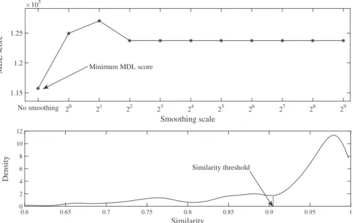
_{. In the top picture of} Fig. 6, the MDL-score as a function of the level of smoothing is indicated. As can be seen, the optimal value for

σ

is 24_{, which} will be the smoothing level used for subsequent landmark extraction and matching with the template.

Based on the landmark constraints and the right smoothing scale, we obtain 245 landmark segments from the smoothed datasets. We continue to evaluate these segments with instance models. For each trust region, there is an instance model cor-responding to it. Our template is marked with 5 landmarks, which can form 10 trust region candidates. In practice, the ﬁrst landmark and the last landmark are sensitive to noise, so we just use the middle three landmarks, which generate 3 trust re-gions. We model each landmark segment based on these trust regions, and select the best-matching model. If the similarity between an obtained instance model and its landmark segment is higher than a given threshold, then the landmark segment will be taken as an instance of the given template. In this case, we choose Pearson’s correlation as the similarity method, and explore the similarity threshold based on the probability density distribution of all similarities. As shown in the bottom picture ofFig. 6, the peak on the left hand side stands for the similarity distribution of true instances, and the index of the changing point (0.918) is taken as the similarity threshold.

Based on the similarity threshold, 221 out of 245 landmark segments are selected as traffic instances. Of these, 20 matches are truck events, corresponding to the 20 trucks identified manually. Of the remaining matches, 161 landmark segments are actual car events (out of the 173 cars), 40 landmark segments are false positives, where sections of noise are recognised as potential cars. The precision of the method is thus 81.9%, and the recall is 93.8%. Note that our recall is 100% for the trucks, which, due to their large size and impact on the strain on the bridge, are much easier to identify than cars. InFig. 7, we plot two features of the manually identified traffic events, demonstrating the case with which trucks can be distinguished

Fig. 5. Traﬃc event detection from a traﬃc dataset. The grey curve in the top picture is a raw dataset collected from a highway bridge; the black curve in the top picture is the smoothed dataset with the smoothing scaleσ=24_{; the solid curve in the bottom left picture is the given template, marked with landmarks A, B,}

C, D and E; the dashed curveDeriv1in the bottom left picture is the ﬁrst derivative curve of the template; the dash-dotted curveDeriv2in the bottom left picture

(11)

Fig. 6. The smoothing scale and similarity threshold of the traﬃc dataset. The top picture shows a scatter plot of the MDL score as a function of smoothing scale, in which the sixth smoothing scale 24_{is selected as the right smoothing scale; the bottom picture shows the probability density distribution of the similarities,}

the changing point 0.918 is selected as the similarity threshold.

0 200 400 600 800 1000 0

2 4 6 8 10

Amplitude

0 50 100

0 0.5 1 1.5

Area

Truck on lane 4

Truck on lane 1

Car on lane 1 Car on lane 4

Noise

Fig. 7. Scatter plot of two features of traffic events. With two features (area and amplitude), traffic event candidates are classified into five groups (noise, car on lane 1, car on lane 4, truck on lane 1, truck on lane 4); the plot indicates that the bounds between noise and car events are blurred.

from cars, as well as traffic-free periods. In the detail in the right of this figure, we note how cars can sometimes be confused with traffic-free periods, due to the level of noise present in the data.Fig. 8 shows two car events in detail, which are clearly hidden by the serious level of noise in the data. Even after being smoothed, the segments are seriously distorted, and cannot be matched with the given template.

6.2. ECG signal

The electrocardiogram (ECG) signal is used to measure the electrical activity of the (human) heart[53]. A single heart beat is typically composed of 5 deﬂections, called the P, Q, R, S and T wave, in which the Q, R and S waves are often considered together as the QRS complex, because they are closely linked. Note that not every QRS complex contains all the three wave elements, and any combination of these waves can also be referred to as a QRS complex[1]. Accurately recognising the QRS complex and distinguishing them from the other noise sources such as P and T waves is a critical technology for many clinical instruments[2].

(12)

Fig. 8.Car events in the traﬃc dataset. This picture shows two car events with a lot of noise, such that it is very hard for a human to even recognise where the car events are.

Fig. 9. The QRS complex detection from an ECG dataset. The grey curve in the top picture is an ECG dataset taken from a real patient; the curve in bottom left picture is a template of QRS complex, which is composed of an R wave and an S wave, and can be marked with 4 landmarks A, B, C and D; in the bottom right picture, black curves stand for matched instance models, and there is also an example of unmatched QRS complex.

lasts 0.06–0.10 s, which is 15–25 data points (at 250 Hz). To be on the safe side, we assume the length of QRS instances ranges between 10 and 30 points. Being the most visually obvious part of ECG signals, the QRS complex features a high R wave and a low S wave, marked asBandCin the template. The amplitude difference betweenBandCvaries with QRS instances, but should also be within a reasonable range. In this experiment, we assume the amplitude range is between 0.2 and 0.8. Based on this prior knowledge, the landmark constraints are set as:

• The length of each landmark subsequence should be 4. • The ﬁrst and third landmarks should be valley points. • The second and the fourth landmarks should be peak points.

• The magnitude of the second landmark should be the highest one in the landmark subsequence. • The magnitude of the third landmark should be the lowest one in the landmark subsequence. • The temporal difference between the last and the ﬁrst landmark should be between 10 and 30. • The magnitude difference between the second and the third landmark should be between 0.2 and 0.8.

(13)

Fig. 10. The smoothing scale and similarity threshold for the ECG dataset. This top picture shows a scatter plot of the MDL score as a function of smoothing scale, and indicates that the ECG dataset need not be smoothed; the bottom picture shows the probability density distribution of the similarities. The changing point 0.901 is selected as the similarity threshold.

left unsmoothed. Based on landmark constraints set above, we manage to catch 142 landmark segments from the original ECG dataset. We continue to detect the similarity threshold with the probability density distribution of the similarities of selected segments. As shown in the bottom picture ofFig. 10, the index of the changing point (0.901) is selected as the similarity threshold. Based on the similarity threshold, 110 out of 142 landmark segments are selected as QRS instances. Of these, 108 are true QRS complexes and 2 are false QRS complexes. The precision of the instance model is thus 90.8%, and the recall is 97.3%.

7. Related work

In this paper, we have presented three concepts that have been extensively used in image matching ﬁelds: templates[5,31], landmarks[31,33]and trust regions[32].

Template matching can be used for face detection[23], duplicate document detection[10]and motion classification[38]. The concept of template has been introduced to time series to detect specific patterns or shapes[18,19,40,41,48]. Frank et al.[18] propose Geometric Template Matching (GeTeM) which uses time-delay embeddings for building models from segments of time series and compares the reconstructed dynamical systems in terms of their state space as well as their dynamics. In[19], a novel and flexible approach is proposed based on segmental semi-Markov models. In[40,41,48], meaningful templates are constructed with shape-based averaging algorithms, such as Prioritized Shape Averaging (PSA)[40]and Accurate Shape Averaging (ASA) [48]. Wei et al. propose the Atomic Wedgie method “that exploits the commonality among the predefined patterns to allow monitoring at higher bandwidths, while maintaining a guarantee of no false dismissals”[56]. Most of the proposed methods are mainly designed for full sequence matching, which are ineffective in detecting predefined patterns from time series.

Landmarks can be used to break time series into meaningful segments, which are also referred to as key-points[8], break-points[47]and change-points[37]. Perng et al.[43]propose a feature-based technique, which uses landmarks instead of the raw data for processing. A two-level representation[8]is proposed to recognise gestures, using both local and global features. In practice, the reliability of each landmark varies with its location. To the best of our knowledge, this has not been mentioned in the literature.

It has been pointed out by researchers that some unspecified portions of time series should be ignored[3,45]to achieve a better matching result, which means some data points have nothing to do with predefined patterns, and should be filtered out. Ye and Keogh[57]propose a new time series primitive, time series shapelets, for time series classification. The shapelets are informally defined as the subsequences that are in some sense maximally representative of a class. This method is interpretable and accurate in classifying static time series[42], but is ineffective in handling real time time series. Inspired by these works, we introduce trust region into time series to obtain more reliable instance models.

(14)

(SAX)[29]and bit-level approximation[7]. Features extracted from time series carry summarised information of the time series [4,55], which can represent the original time series concisely[21], and are less sensitive to noise[39], so the feature extraction operation can also be used to reduce dimensionality (reduce the size of the data), such as Amplitude-Level Features (ALF)[6], Characteristic-based Clustering (CBC)[55]. Some representations are based on piecewise techniques, such as Piecewise Linear Approximation (PLA)[47], Piecewise Aggregate Approximation (PAA)[25], Adaptive Piecewise Constant Approximation (APCA) [11], Derivative Time Series Segment Approximation (DSA)[21]and Piecewise Vector Quantized Approximation (PVQA)[34,54]. Some representations aim to keep both local and global information about the original time series, such as Multi-resolution Vector Quantization (MVQ) approximation[35]and multi-resolution PAA (MPAA)[30].

Next to the representation methods, a number of similarity measures have been proposed[16], of which the Euclidean Dis-tance (ED)[17,58]is the most common[4,15]. However, when shifting and temporal distortions exist in the given time series, the ED is proven to be ineffective[15]. To handle stretching and compression along the temporal dimension, Dynamic Time Warp-ing (DTW)[9]was proposed, which achieves an optimal temporal alignment through detecting the shortest warping path in a distance matrix[16,41,44,48]. Finding the shortest warping path is a non-trivial problem, whose computation complexity can reachO

(

n2

₎

_{, where}_n_{is the number of data points. To speed up the computation of DTW, some lower bounding constraints, like} LB_Keogh[24,44]and the Ratanamahatana-Keogh Band[46], have been introduced to prune expensive computations, which can reduce the complexity toO

(

n

)

. There are also some other edit-based methods proposed to handle outliers and noise[16], such as Longest Common Subsequence (LCSS)[52], Edit Distance with Real Penalty (ERP)[13]and Edit Distance on Real sequence (EDR) [14]. However, most of the proposed methods focus mainly on temporal deformations[19], which are inadequate in dealing with shifting and scaling in the amplitude dimension[15]. Consequently, Spatial Assembling Distance (SpADe)[15]is proposed to handle shifting and scaling in both the temporal and amplitude dimensions.

8. Conclusion

Predefined pattern detection from time series is a quite challenging topic, because it is not only sensitive to noise, but also sensitive to temporal and magnitude deformations. A number of representation and similarity measure methods have been proposed to approximate interesting subsequences, but most of them are mainly designed for full sequence matching, and are ineffective when the disturbances mentioned above exist. We refer a predefined pattern as a template, and featured it with a sequence of landmarks (important points). Instead of comparing the template with subsequences of a given times series, we first transfer the time series into a landmark sequence, and compare the template landmark sequence with the time series landmark subsequences. The landmark constraints derived from the template and prior knowledge play a key role in finding matched landmark subsequences and landmark segments. We model the landmark segments with the template, and obtain a number of instance models. If the similarity between a landmark segment and its instance model is above a threshold, then the segment will be taken as an instance of the template. We introduce advanced methods, like MDL and PDF, to set important parameters, such as smoothing scale and similarity threshold. Most of the existing feature-based methods just focus on the quality of models, and pay little attention to the reliability of candidate patterns. Our instance model overcomes this problem by transferring the template in both temporal and magnitude dimensions according to trust regions.

Acknowledgments

This work and the InfraWatch project are funded by the Dutch funding agency (STW), under Project No. 10970.

References

[1] 2014.<http://en.wikipedia.org/wiki/QRS_complex>.

[2] V.X. Afonso, ECG QRS detection, Biomedical Digital Signal Processing: C-language Examples and Laboratory Experiments for the IBM PC, 1993, pp. 236–264. [3] R. Agrawal, K. Lin, H. Sawhney, K. Shim, Fast similarity search in the presence of noise, scaling, and translation in time-series databases, in: Proceedings of

International Conference on Very Large Databases, 1995, pp. 490–501.

[4] R.J. Alcock, Y. Manolopoulos, Time-series similarity queries employing a feature-based approach, in: Proceedings of Hellenic Conference on Informatics, 1999, pp. 27–29.

[5] Y. Amit, U. Grenander, M. Piccioni, Structural image restoration through deformable templates, J. Am. Stat. Assoc. 86 (1991) 376–387.

[6] J. Aßfalg, H.-P. Kriegel, P. Kröger, P. Kunath, A. Pryakhin, M. Renz, Similarity search in multimedia time series data using amplitude-level features, in: Proceedings of International Conference on Advances in Multimedia Modeling, 2008, pp. 123–133.

[7] A. Bagnall, C. Ratanamahatana, E. Keogh, S. Lonardi, G. Janacek, A bit level representation for time series data mining with shape based similarity, Data Min. Knowl. Discov. 13 (2006) 11–40.

[8] J.P. Bandera, R. Marﬁl, A. Bandera, J.A. Rodríguez, L. Molina-Tanco, F. Sandoval, Fast gesture recognition based on a two-level representation, Pattern Recogn. Lett. 30 (2009) 1181–1189.

[9] D.J. Berndt, J. Clifford, Using dynamic time warping to ﬁnd patterns in time series, in: Proceedings of KDD Workshop, 1994, pp. 359–370. [10]R. Caprari, Duplicate document detection by template matching, Image Vision Comput. 18 (8) (2000) 633–643.

[11]K. Chakrabarti, E. Keogh, S. Mehrotra, M. Pazzani, Locally adaptive dimensionality reduction for indexing large time series databases, ACM Trans. Database Syst. 27 (2) (2002) 188–228.

(15)

[14] L. Chen, M.T. Özsu, V. Oria, Robust and fast similarity search for moving object trajectories, in: Proceedings of International Conference on Management of Data, 2005, pp. 491–502.

[15] Y. Chen, M. Nascimento, B. Ooi, A. Tung, Spade: on shape-based pattern detection in streaming time series, in: Proceedings of International Conference on Data Engineering, 2007, pp. 786–795.

[16] P. Esling, C. Agon, Time-series data mining, ACM Comput. Surv. (CSUR) 45 (1) (2012) 12:1–12:34.

[17] C. Faloutsos, M. Ranganathan, Y. Manolopoulos, Fast subsequence matching in time-series databases, in: Proceedings of the International Conference on Management of Data, 1994, pp. 419–429.

[18] J. Frank, S. Mannor, J. Pineau, D. Precup, Time series analysis using geometric template matching, IEEE Trans. Pattern Anal. Machine Intell. 35 (3) (2013) 740–754.

[19] X. Ge, P. Smyth, Deformable markov model templates for time-series pattern matching, in: Proceedings of International Conference on Knowledge Discovery and Data Mining, 2000, pp. 81–90.

[20] P.D. Grünwald, The Minimum Description Length Principle, The MIT Press, 2007.

[21]F. Gullo, G. Ponti, A. Tagarelli, S. Greco, A time series representation model for accurate and fast similarity detection, Pattern Recogn. 42 (2009) 2998–3014. [22] B. Hu, T. Rakthanmanon, Y. Hao, S. Evans, S. Lonardi, E. Keogh, Discovering the intrinsic cardinality and dimensionality of time series using MDL, in:

Pro-ceedings of International Conference on Data Mining, 2011, pp. 1086–1091.

[23] Z. Jin, Z. Lou, J. Yang, Q. Sun, Face detection using template matching and skin-color information, Neurocomputing 70 (4–6) (2007) 794–800. [24] E. Keogh, Exact indexing of dynamic time warping, in: Proceedings of International Conference on Very Large Data Bases, 2002, pp. 406–417.

[25] E. Keogh, K. Chakrabarti, M. Pazzani, S. Mehrotra, Dimensionality reduction for fast similarity search in large time series databases, Knowl. Inform. Syst. 3 (2001) 263–286.

[26] E. Keogh, Q. Zhu, B. Hu, Y. Hao, X. Xi, L. Wei, C.A. Ratanamahatana, The UCR time series classiﬁcation/clustering page, 2011.<http://www.cs.ucr.edu/eamonn/ time_series_data/>.

[27] A. Knobbe, H. Blockeel, A. Koopman, T. Calders, B. Obladen, C. Bosma, H. Galenkamp, E. Koenders, J. Kok, Infrawatch: data management of large systems for monitoring infrastructural performance, in: Proceedings of Intelligent Data Analysis, 2010, pp. 91–102.

[28] F. Korn, H.V. Jagadish, C. Faloutsos, Eﬃciently supporting ad hoc queries in large datasets of time sequences, in: Proceedings of International Conference on Management of Data, 1997, pp. 289–300.

[29] J. Lin, E. Keogh, S. Lonardi, B. Chiu, A symbolic representation of time series, with implications for streaming algorithms, in: Proceedings of ACM SIGMOD Workshop on Research Issues in Data Mining and Knowledge Discovery, 2003, pp. 2–11.

[30] J. Lin, M. Vlachos, E. Keogh, D. Gunopulos, J. Liu, S. Yu, J. Le, A MPAA-based iterative clustering algorithm augmented by nearest neighbors search for time-series data streams, in: Proceedings of Paciﬁc-Asia Conference on Knowledge Discovery and Data Mining, 2005, pp. 333–342.

[31] R. Liu, Y. Lu, C. Gong, Y. Liu, Infrared point target detection with improved template matching, Infrared Phys. Technol. 55 (4) (2012) 380–387. [32] T. Liu, H. Chen, Real-time tracking using trust-region methods, IEEE Trans. Pattern Anal. Machine Intell. 26 (3) (2004) 397–402.

[33] M. Lüthi, C. Jud, T. Vetter, Using landmarks as a deformation prior for hybrid image registration, in: Proceedings of International Conference on Pattern Recognition, 2011, pp. 196–205.

[34] V. Megalooikonomou, G. Li, Q. Wang, A dimensionality reduction technique for eﬃcient similarity analysis of time series databases, in: Proceedings of International Conference on Information and Knowledge Management, 2004, pp. 160–161.

[35] V. Megalooikonomou, Q. Wang, G. Li, C. Faloutsos, A multiresolution symbolic representation of time series, in: Proceedings of International Conference on Data Engineering, 2005, pp. 668–679.

[36] S. Miao, E. Koenders, A. Knobbe, Automatic baseline correction of strain gauge signals, Struct. Control Health Monit. 22 (2015) 36–49. [37]Y. Mohammad, T. Nishida, Constrained motif discovery in time series, New Gener. Comput. 27 (2009) 319–346.

[38] M. Müller, T. Röder, Motion templates for automatic classiﬁcation and retrieval of motion capture data, in: Proceedings of ACM SIGGRAPH/Eurographics Symposium on Computer Animation, 2006, pp. 137–146.

[39] A. Nanopoulos, R. Alcock, Y. Manolopoulos, Feature-based classiﬁcation of time-series data, Int. J. Comput. Res. 10 (2001) 49–61.

[40] V. Niennattrakul, C. Ratanamahatana, Shape averaging under time warping, in: Proceedings of International Conference on Electrical Engineer-ing/Electronics, Computer, Telecommunications, and Information Technology, 2009, pp. 626–629.

[41] V. Niennattrakul, D. Srisai, C. Ratanamahatana, Shape-based template matching for time series data, Knowl.-Based Syst. 26 (2012) 1–8.

[42] T. Palpanas, M. Vlachos, E. Keogh, D. Gunopulos, W. Truppel, Online amnesic approximation of streaming time series, in: Proceedings of International Conference on Data Engineering, 2004, pp. 338–349.

[43] C.-S. Perng, H. Wang, S.R. Zhang, D.S. Parker, Landmarks: a new model for similarity-based pattern querying in time series databases, in: Proceedings of International Conference on Data Engineering, 2000, pp. 33–42.

[44] T. Rakthanmanon, B. Campana, A. Mueen, G. Batista, B. Westover, Q. Zhu, J. Zakaria, E. Keogh, Searching and mining trillions of time series subsequences under dynamic time warping, in: Proceedings of International Conference on Knowledge Discovery and Data Mining, 2012, pp. 262–270.

[45] T. Rakthanmanon, E. Keogh, S. Lonardi, S. Evans, Time series epenthesis: Clustering time series streams requires ignoring some data, in: Proceedings of International Conference on Data Mining, 2011, pp. 547–556.

[46] C. Ratanamahatana, E. Keogh, Making time-series classiﬁcation more accurate using learned constraints, in: Proceedings of SIAM International Conference on Data Mining, 2004, pp. 11–22.

[47] H. Shatkay, S. Zdonik, Approximate queries and representations for large data sequences, in: Proceedings of International Conference on Data Engineering, 1996, pp. 536–545.

[48] D. Srisai, C. Ratanamahatana, Eﬃcient time series classiﬁcation under template matching using time warping alignment, in: Proceedings of International Conference on Computer Sciences and Convergence Information Technology, 2009, pp. 685–690.

[49] U. Vespier, A. Knobbe, S. Nijssen, J. Vanschoren, MDL-based analysis of time series at multiple time-scales, in: Proceedings of European Conference on Machine Learning and Principles and Practice of Knowledge Discovery in Databases, 2012, pp. 371–386.

[50] U. Vespier, A. Knobbe, J. Vanschoren, S. Miao, A. Koopman, B. Obladen, C. Bosma, Traﬃc events modeling for structural health monitoring, in: Proceedings of Intelligent Data Analysis, 2011, pp. 376–387.

[51] U. Vespier, S. Nijssen, A. Knobbe, Mining characteristic multi-scale motifs in sensor-based time series, in: Proceedings of International Conference on Information and Knowledge Management, 2013, pp. 2393–2398.

[52] M. Vlachos, D. Gunopoulos, G. Kollios, Discovering similar multidimensional trajectories, in: Proceedings of International Conference on Data Engineering, 2002, pp. 673–684.

[53] G. Walraven, Basic Arrhythmias, Prentice Hall, 2010.

[54] Q. Wang, V. Megalooikonomou, A dimensionality reduction technique for eﬃcient time series similarity analysis, Inform. Syst. 33 (2008) 115–132. [55] X. Wang, K. Smith, R. Hyndman, Characteristic-based clustering for time series data, Data Min. Knowl. Discov. 13 (2006) 335–364.

[56] L. Wei, E. Keogh, H. Van Herle, A. Mafra-Neto, Atomic wedgie: Eﬃcient query ﬁltering for streaming times series, in: Proceedings of International Conference on Data Mining, 2005, pp. 490–497.

[57] L. Ye, E. Keogh, Time series shapelets: A new primitive for data mining, in: Proceedings of International Conference on Knowledge Discovery and Data Mining, 2009, pp. 947–956.