Computational video enhancement

(1)

COMPUTATIONAL VIDEO ENHANCEMENT

Eric P. Bennett

A dissertation submitted to the faculty of the University of North Carolina at Chapel Hill in partial fulfillment of the requirements for the degree of Doctor of Philosophy in the Department of Computer Science.

Chapel Hill 2007

Approved by:

Leonard McMillan

Gary Bishop

Guido Gerig

Sing Bing Kang

Marc Pollefeys

(2)

c

2007

(3)

ABSTRACT

ERIC P. BENNETT: Computational Video Enhancement (Under the direction of Leonard McMillan)

During a video, each scene element is often imaged many times by the sensor. I propose

that by combining information from each captured frame throughout the video it is possible

to enhance the entire video. This concept is the basis of computational video enhancement.

In this dissertation, the viability of computational video processing is explored in addition to

presenting applications where this processing method can be leveraged.

Spatio-temporal volumes are employed as a framework for efficient computational video

processing, and I extend them by introducing sheared volumes. Shearing provides spatial

frame warping for alignment between frames, allowing temporally-adjacent samples to be

pro-cessed using traditional editing and filtering approaches. An efficient filter-graph framework

is presented to support this processing along with a prototype video editing and manipulation

tool utilizing that framework.

To demonstrate the integration of samples from multiple frames, I introduce methods

for improving poorly exposed low-light videos to achieve improved results. This integration is guided by a tone-mapping process to determine spatially-varying optimal exposures and

an adaptive spatio-temporal filter to integrate the samples. Low-light video enhancement is

also addressed in the multispectral domain by combining visible and infrared samples. This

is facilitated by the use of a novel multispectral edge-preserving filter to enhance only the

visible spectrum video.

Finally, the temporal characteristics of videos are altered by a computational video

re-sampling process. By rere-sampling the video-rate footage, novel time-lapse sequences are found

that optimize for user-specified characteristics. Each resulting shorter video is a more

faith-ful summary of the original source than a traditional time-lapse video. Simultaneously, new

(4)

To My Father, Robert A. Bennett,

(5)

ACKNOWLEDGMENTS

I would like to thank my advisor, Leonard McMillan, for working with me for five years and

guiding my development as a researcher. I will certainly miss our enthusiastic brainstorming

sessions, where Leonard’s drive to explore the limits of computer science was most evident.

I would also like to thank the rest of my committee: Gary Bishop, Guido Gerig, Sing

Bing Kang, Marc Pollefeys, and Carlo Tomasi. I am honored to have such a distinguished

committee and I appreciate their time and feedback on my work.

I want to thank John Mason for the multispectral datasets in Section 4.3 as well as Aaron

Block, Tim Malone, Terry McMahon, and John Moriconi for appearing in my videos.

My thanks as well to my collaborators on projects outside of this dissertation: Jason

Stewart, Jingdan Zhang, Sing Bing Kang, Rick Szeliski, Matt Uyttendaele, and Larry Zitnick.

Discussions with friends and colleagues at UNC have also influenced my work: Aaron Block, Dave Borland, Fred Brooks, Brian Eastwood, Russ Gayle, Justin Hensley, Tyler

Johnson, Luv Kohli, Anselmo Lastra, E. Scott Larsen, Brandon Lloyd, Ketan Mayer-Patel,

Chris Oates, Rick Skarbez, Josh Steinhurst, Russell Taylor, Chris VanderKnyff, Jeremy

Wendt, Jingyi Yu, and many more. Thanks also to my friends from around the country:

Derek Jarvis, Zac Johnson, Liz Koster, John Moriconi, and Zak Vassar.

Finally, I would like to thank my parents, Robert and Marilyn, for being such wonderful

inspirations throughout my life. Both teachers, they instilled in me a deep appreciation for

eduction I have since carried with me. I dedicated this work to my father for being the Ph.D.

role model I have always aspired to and also for introducing me to the wonders of computer

technology, going all the way back to the TI-99/4A and later including some of the first digital

video editors. Finally, thanks to my brother Rob and his wife Kristie for their support (and

(6)

LIST OF TABLES

4.1 VEC example video statistics . . . 69

4.2 Table of LDR input video statistics . . . 70

4.3 VEC post-processing statistics . . . 70

(11)

LIST OF FIGURES

1.1 Spatio-temporal volume visualized as planes . . . 3

2.1 Images comparing Gaussian and bilateral decompositions . . . 13

2.2 Comparison of existing spatial filtering techniques . . . 15

2.3 Additional comparison of existing spatial filtering techniques . . . 16

2.4 Tone mapping pipeline of Durand and Dorsey (2002) . . . 21

3.1 Screenshot of an 8 second spatio-temporal video volume . . . 29

3.2 Spatio-temporal volume visualized as a solid . . . 30

3.3 Spatio-temporal cut plane . . . 31

3.4 Shearing of a spatio-temporal volume . . . 32

3.5 Spatio-temporal volume showing neighborhood interaction . . . 33

3.6 Illustration of the shearing process . . . 35

3.7 PFilter interconnections in a Proscenium filter graph . . . 37

3.8 Proscenium pixel query ordering . . . 38

3.9 A Proscenium filter graph for edge color tinting. . . 39

3.10 Proscenium video editing application architecture . . . 42

3.11 Two frames from a Frisbee throwing video . . . 44

3.12 Stabilized Frisbee video visualization . . . 45

3.13 Stabilized Frisbee video frames . . . 45

(12)

3.15 Before and after widening the aspect ratio of the Frisbee sequence. . . 46

3.16 Temporal painting of a walking teapot video . . . 47

4.1 A teapot video frame processed using the Virtual Exposure Camera . . . 53

4.2 The Virtual Exposure Camera model . . . 53

4.3 Bilateral filter shot noise processing . . . 56

4.4 Illustration of the spatial neighborhood dissimilarity value . . . 59

4.5 Illustration of the ASTA filter’s adaptive kernel . . . 61

4.6 Flowchart of the entire VEC process . . . 63

4.7 Plots of the non-linear mapping function . . . 64

4.8 A frame of video (forest) processed using the VEC . . . 67

4.9 A frame of video (hand) processed using the VEC . . . 67

4.10 Color histograms during VEC processing . . . 68

4.11 Four example LDR videos . . . 69

4.12 Plot of SNR for four videos . . . 71

4.13 Plot of luminance distribution for four videos . . . 72

4.14 Illustration of the prototype multispectral imaging setup . . . 74

4.15 Illustration of the luminance processing of the fusion technique . . . 75

4.16 Comparison of image decomposition methods . . . 81

4.17 Images at various stages of multispectral fusion . . . 82

(13)

4.19 Fusion results from walking person video . . . 86

4.20 Fusion results from dancing robot video . . . 87

4.21 Photograph of multispectral capture setup . . . 87

4.22 Comparison of multispectral fusion mean spatial variances . . . 88

4.23 Joint bilateral versus dual bilateral comparison . . . 89

5.1 Sequences of time-lapse frames illustrating video aliasing . . . 92

5.2 Diagram of the data flow within the computational time-lapse video system. . 93

5.3 1D Plots of uniform and non-uniform samplings . . . 100

5.4 Illustration of the virtual shutter exposure window . . . 104

5.5 Unprocessed time-lapse input frames . . . 107

5.6 Video of car headlights extended with virtual exposures . . . 109

5.7 Multiple virtual shutters processing video of a car defrosting . . . 111

5.8 Resulting samplings of test videos . . . 112

5.9 Two examples of dense motion tails . . . 113

A.1 PFilter class structure and components . . . 120

A.2 PShear video volume shearing . . . 125

(14)

LIST OF ABBREVIATIONS

1D One-Dimensional

2D Two-Dimensional

3D Three-Dimensional

ACM Association for Computing Machinery

A/D Analog to Digital

ADC Analog to Digital Converter

API Application Programming Interface

ASTA Adaptive Spatio-Temporal Accumulation

AVI Audio Video Interleave

CCD Charge-Coupled Device

CMOS Complementary Metal-Oxide-Semiconductor

codec Compression/Decompression

CPU Central Processing Unit

DLP Digital Light Processing

DV Digital Video

FAQ Frequently Asked Questions

FIFO First In, First Out

fps Frames Per Second

GB Gigabyte

GHz Gigahertz

GPU Graphics Processing Unit

HDR High Dynamic Range

IEEE Institute of Electrical and Electronics Engineers

InGaAs Indium Gallium Arsenide

IR Infrared

LCD Liquid Crystal Display

(15)

LED Light-Emitting Diode

LS Large-Scale

LSI Linear Spatially/Shift Invariant

MiniDV Miniature Digital Video (IEC 61834)

NIR Near Infrared

nm Nanometer

NTSC National Television Systems Committee

OpenCV Open Source Computer Vision Library

OpenGL Open Graphics Library

PAL Phase Alternating Line

PC Personal Computer

PFilter Proscenium Filter

RAM Random Access Memory

RGB Red Green Blue

RGBα Red Green Blue Alpha

ROAD Rank-Order Absolute Difference

s Second

µs Microsecond

SAD Sum-of-Absolute-Differences

SIGGRAPH Special Interest Group on Graphics and Interactive Techniques

SNR Signal-To-Noise Ratio

SSD Sum-of-Squared-Differences

SUSAN Smoothing over Univalue Segment Assimilating Nucleus

SWIR Short Wave Infrared

VEC Virtual Exposure Camera

(16)

CHAPTER 1

INTRODUCTION

The popularity of digital video camcorders has ushered in a desktop digital video revolution

for both professional and amateur users. High quality video can be captured, imported, and

processed on commodity computers at minimal cost and with unprecedented ease. Having

such video available on a computer lends itself to traditional video editing applications. Thus,

along with the availability of digital video hardware came software editing tools of varying

complexities for many different skill levels. However, these tools focused primarily on the

temporal rearrangement of short video clips as they were imaged. The problem of making the

underlying footage better, to significantly improve its visual quality and enhance its content,

presents the next challenge and opportunity for digital video.

I first consider traditional video processing approaches for enhancing the quality of video.

Simple tasks such as the global adjustment of brightness, contrast, color balance, and other

characteristics are all well understood and are the limit of functionality in most video editors.

Few local enhancements, such as noise reduction, are available and those that are offered are

typically simple linear filters considering at most na¨ıve frame-by-frame filtering or very small temporal neighborhoods, being an outgrowth of analog processing. However, with modern

digital hardware and random access to all pixels in all video frames simultaneously, far more

complex, adaptive, and non-linear approaches can now be taken that require the storage and

computational power that has only recently become available.

When considering the possibilities of such processing, it is worthwhile to consider

simi-lar work on still images. Specifically, the field of computational photography addresses the

enhancement of still images by considering information in a small number of similar images

(17)

together with computational methods, a image superior to anything possible to capture with

a physical camera is created. For instance, visual elements that appear in only one image

may be combined with visual elements from other images taken minutes apart to create a realistic composite image. Or, images taken at different exposures allow a combined image

with dynamic range beyond that of the sensor to be computed. Lighting may be transferred,

noise reduced, spectra fused, or many other effects not possible in-camera that leverage both

computation and the fact that many images can be taken at no additional cost.

Bringing the benefits of computational photography to traditional video processing, the

emerging field of computational video addresses combining elements between frames to

gen-erate an enhanced video output. Computational video has vast potential because so much

information is available for processing when capturing at video rates. For example, at 30

frames per second, 1,800 individual frames are captured every minute, and 108,000 frames

are captured every hour.

Along with this additional data comes new issues that uniquely arise in computational

video in comparison to computational photography. First, the output is a video sequence

as opposed to a single frame. Thus, frame-to-frame enhancement decisions must be made

consistently so they do not introduce artifacts when played back at full speed (temporal

coherence). Second, the number of input images makes identification of the most useful

information difficult. In addition, the infrastructure and underlying data structures must be

able to support the increased quantity of data.

Overcoming these issues enables many powerful new video tools. Tasks such as video

compositing and object removal can be performed in a temporally coherent manner. Videos

may be adaptively filtered and enhanced using large kernels that span space, time, and even

across multiple spectra. The linear progression of time can be altered and resampled to change

the underlying structure of the original video.

Thus, given this potential of computational video, my thesis statement is:

Computational video enables a new class of processing tools for

enhancing and improving video capture quality by leveraging

(18)

1.1 Contributions

My research makes the following contributions:

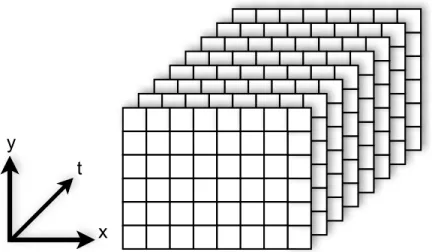
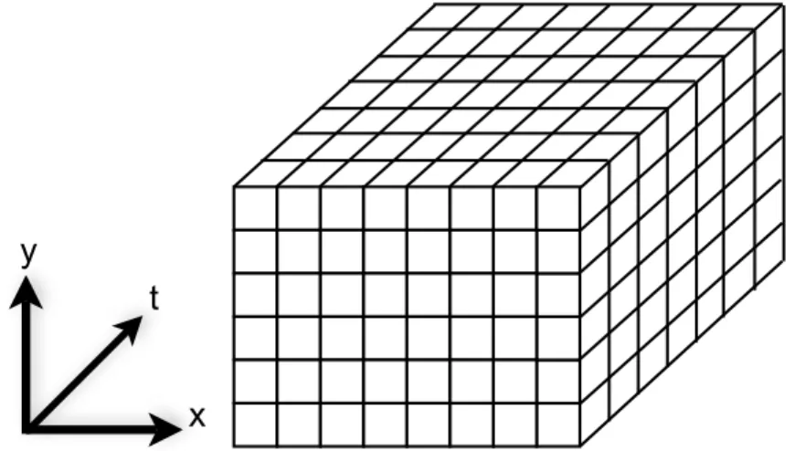
• I employ spatio-temporal video volumes as a domain for computational video operations

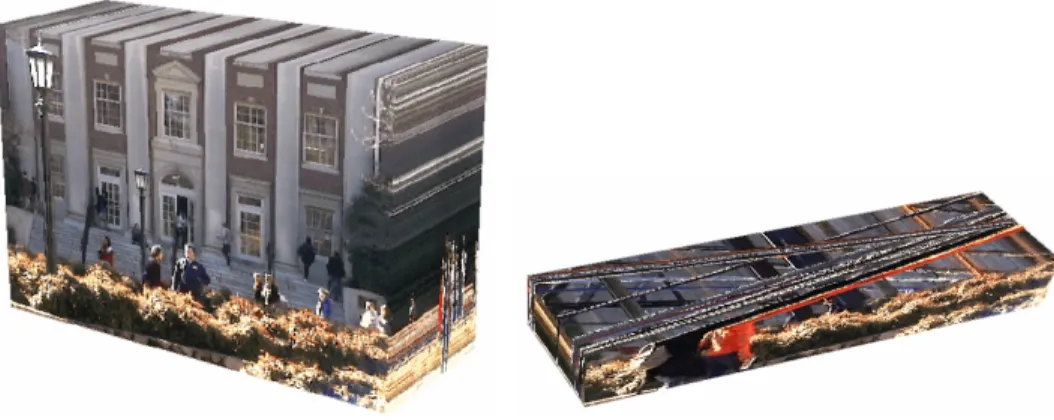
and extend them with shearing. Spatio-temporal volumes stack the frames of a video

in chronological order to create a 3D volume, as shown in Figure 1.1, thus emphasizing

relationships between adjacent spatial and temporal samples. Shearing is the process

of spatially warping the frames of the volume to align temporally-adjacent samples to greatly assist the processing of moving objects and non-static cameras.

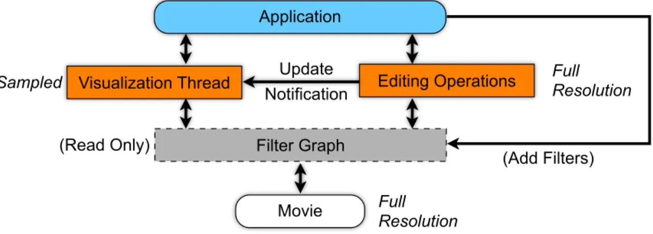
• I develop the Proscenium spatio-temporal video editing framework to address the

mem-ory and processing requirements of computational video and spatio-temporal volumes.

This framework encapsulates spatio-temporal volumes within aper-pixel, bi-directional,

lazily-evaluated filter graph model. This model also supportsvirtual shears that can be

created and removed dynamically to support editing. This framework is then used to

develop a prototype video editor that performs computational video manipulation tasks

such as object removal, temporal filtering, and multi-frame editing.

• I present a computational video approach to improving the quality of captured low-light,

LDR (Low Dynamic Range) video by virtually extending the exposure times of each

x

y

t

(19)

sample (pixel). This is possible with the non-linear integration of information from

large neighborhoods of temporally and spatially adjacent samples. Two interconnected

concepts make this possible. First is a spatially-varying LDR tone mapping algorithm

that finds the optimal exposure time in a well-exposed image. This is used as an

ob-jective for theintegration and noise reduction ASTA (Adaptive Spatio-Temporal

Accu-mulation) filterwhich extends the exposure time to find the correct original luminance

had it been properly exposed. When used together, this combined method is referred

to as theVirtual Exposure Camera model.

• To improve captured video in a different context,I also address enhancing low-light video

using spectra outside of the standard visible red, green, and blue channels. Specifically,

information from registered video in the IR spectrum is used to enhance noisy RGB

footage. My approach differs from previous multispectral fusions because it enhances the

RGB footage using the IR, but without introducing elements imaged only in IR. This is

accomplished through edge-preserving decomposition and cross-spectral normalization,

assisted by a novel dual bilateral filter. This filter preserves edges detected in both

spectra but only uses samples from the visible-spectrum video.

• Having considered video manipulation and enhancement as examples of computational

video,I then consider temporal resampling of videos to alter their duration. Specifically,

the problem of time-lapse video generation from video-rate footage is considered. A

non-uniform sampling algorithm is presented that optimizes the sampling of the input

video to match the user’s desired duration and visual output characteristics. This can

be either to generate time-lapse videos that preserve motion, avoid fast motion, control

the uniformity of the output sampling, or a combination of these characteristics. By

considering the entire video as a whole, the optimal sampling can be found.

• To complement the computational video resampling,I extend ideas from computational

photography to combine the input frames together to alter the aliasing characteristics of

the video output. Thisvirtual shutter combines many frames together using both

(20)

median filtering, and more complex effects, such as compositing. Thus, new synthetic

exposures are created which are related to both the low-light ASTA exposures and the

spatio-temporal filtering performed in Proscenium.

1.2 Dissertation Overview

My approaches to computational video are presented as follows:

To begin, the field of computational video will be reviewed in Chapter 2. Because this

field is an outgrowth of image processing, video processing, and computational photography,

relevant topics from those areas are discussed as well.

In Chapter 3, the use of spatio-temporal volumes for computational video processing is

examined. This is presented along with volume shearing, the Proscenium spatio-temporal video editing framework, and discussion of how computational video operations, in this case

video editing and enhancement, can be performed within these volumes.

In Chapter 4, a computational approach to video enhancement is discussed for improving

the quality of noisy low-light videos, showing the strengths of adaptive filtering with large

spatio-temporal kernels. Visible-spectrum-only enhancement is discussed, with the Virtual

Exposure Camera model, combining LDR tone mapping and the ASTA filter. Multi-spectral

video enhancement is then addressed with a focus on the new dual bilateral filter.

In Chapter 5, a computational video approach to video resampling and frame combination

is presented to shorten the duration of videos into time-lapse sequences. This demonstrates the

ability of computational video to dramatically alter the content of an input video. The sampler

is presented along with a variety of metrics to achieve many output sampling characteristics.

The output frames are then generated by the virtual shutter that combines all the frames in

the original video using linear and non-linear techniques.

(21)

CHAPTER 2

PREVIOUS WORK

In this chapter, I provide an overview of the previous literature regarding computational video.

Computational video is an outgrowth of video processing and computational photography,

both of which are based on image processing. Thus, to consider computational video is

to consider each of these component fields. Specifically, the common thread through this

discussion is that the potential of computational video is derived from its ability to enhance

the samples in a video by combining observations from other similar frames.

I begin this literature review by considering the established methods for processing digital

video: traditional video editors and video processing frameworks. I then review recent work

in spatio-temporal volumes, which present an alternate representation of video that lends

itself to filtering and enhancement applications. Further investigation of traditional filtering

is then discussed in the context of the classic image processing area of noise reduction. The

focus then shifts to computational photography, specifically in the domains of High Dynamic

Range (HDR) imaging, multispectral fusion, and multi-image combination. Given all this

work as a basis, computational video is then considered, addressing both the summarization and compositing of video sources.

2.1 Video Editing

The most common interface for processing or enhancing video is through a dedicated video

editing application. Therefore, I begin by discussing the goals of these applications along

with those of the low-level frameworks often used to encapsulate video processing.

The primary function of most modern digital video editing systems, such as Apple Final

(22)

clips, and then assemble those clips with transitions along some timeline into a finished video.

Such editors perform cuts, cropping, editing, color-correction, and insertion of transitions

be-tween clips. Applications such as Adobe After Effects focus on making modifications primarily on individual clips (often a few seconds long). These modifications are often more complex

and concentrate on the modification of video pixels and less on temporal arrangement. These

operations are closer to the type of actions considered by computational video.

The visual interface used for interaction in all of these applications is a timeline plus

a frame-by-frame viewer. Thus time and space dimensions are treated inherently different

from each other. This does not lend itself well to the incorporation of samples and other

elements from multiple frames that are necessary for computational video. Alternate

repre-sentations, such as 3D spatio-temporal volumes, discussed in Chapter 3, consider the entirety

of a video at once. However, there have been recent efforts in mixing standard 2D image

editing user-interface metaphors with such 3D visualizations. Ideas from Adobe Photoshop,

a popular commercial image-editing tool, are, in fact, frequently applied to both 3D and video

applications because of its ease of use, flexibility, and rich set of tools. Furthermore, systems

have been proposed to extend Photoshop’s rich image-editing environment to volumetric data

(Zwicker et al., 2002). By extension, such techniques may hold promise for processing video in spatio-temporal volumes.

Many video processing systems are based upon filter graphs which have been utilized for

many applications in the area of image and multimedia processing (Pratt, 1997).

Conceptu-ally, the idea is that individual processing components can be ordered and arranged so that

data flows from the input of a filter graph to the output; passing through the interconnected

components that lie along that path. Each component (often called a filter) may modify data

before passing it along to the next filter. Each filter is only responsible for processing data

in a standardized manner without knowledge of what filters might be connected to it. This

allows a uniform interface with components that are interconnected in any order, as in the

Decorator design pattern (Gamma et al., 1995). These filters are often representative of the

common operations that occur throughout video editing: color correction, smoothing, scaling,

(23)

For instance, Apple’s QuickTime (Apple Inc., 2007) framework and Microsoft’s

Direct-Show (Microsoft Corporation, 2007) framework implement multimedia filter graphs for video

and audio. At a higher level of abstraction, the Berkeley Continuous Media Toolkit (Mayer-Patel and Rowe, 1997) implements a powerful filter graph in the form of a scripting protocol,

as opposed to a compiled API. Filter graphs treat video data as a stream that flows in buffers

of entire frames of pixels from the graph’s input to the graph’s output. This is ideal when an

entire frame’s output is desired, but is not ideal to calculate small sub-frame regions.

As mentioned, the frame-by-frame timeline nature of these video editors and frameworks

differs from the needs of computational video to consider many frames simultaneously for

enhancement. Thus, a different method for thinking about video, the spatio-temporal volume,

is now discussed.

2.2 Spatio-Temporal Volumes

Considering videos as three-dimensional volumes of their stacked constituent frames was first

proposed in the epipolar video processing research of Bolles et al. (1987). In this work, object

and scene motion are measured by taking a planarcutof a spatio-temporal volume containing

the video. Each cut results in a still image that contains portions of many frames, allowing

for correlations to be made in 2D between position and time to measure object velocity. An

underlying assumption of these measurements is that the camera that captured the source

video was static so that spatial positions in the video are constant through time.

These volumes and planar cuts were later realized as an interactive visualization in

“Inter-active Video Cubism” (Fels et al., 2000). These spatio-temporal cuts (originally planar and

later spherical) again provide a view into the video, but do not modify the underlying data.

More advanced applications are then explored in (Klein et al., 2001) and (Klein et al., 2002),

which both use multiple spatio-temporal cuts to create artistic video interpretations of the source material. In an extreme case, “Making Space For Time in Time-Lapse Photography”

(Terry et al., 2004) scales the cut plane concept to visualize the total contents of multiple

days of video footage in a single image. Alternatively, Zomet et al. (2003) identified

(24)

different from the projection of the imaging device. These works demonstrate a wide range

of visualizations that motivate the possibilities of spatio-temporal processing.

The spatial-alignment of individual frames is essential to video processing within a spatio-temporal volume. As will be further discussed in Section 3.1, this alignment guarantees that

a consistent spatial pixel location in the volume is always imaging the same scene element.

Thus, enhancement algorithms can access other samples of the same object at the same

(x, y) coordinate but at different tvalues (time). I call this spatial remapping of the volume

shearing. Planar cuts of a sheared volume represent non-planar cuts of the original

spatio-temporal volume. Non-planar spatio-spatio-temporal cuts have since been used as an interface to

specify multi-frame compositing operations (Wang et al., 2005).

It follows then that the parameters for shearing are derived from stabilizing a scene element

through time. Shearing can be used to stabilize each element one-at-a-time, allowing each

visual element to be edited, processed, or enhanced independently. This approach is influenced

by the video layers concepts of Wang and Adelson (1994) who developed the notion that

general planes of motion in a video should be edited independently.

To solve for a spatio-temporal volume’s underlying shear function, a variety of

stabi-lization methods exist. Buehler et al. (2001) demonstrate how foreground and background stabilization can be used to generate novel videos with refined camera and object motions.

Their work relies on extensive offline analysis for dense feature tracking, local warping, and

iterative smoothing of the source sequence. More recently, Sand and Teller (2004) presented

a “Video Matching” method for aligning slightly different video sources. This alignment is

between videos, and is able to robustly handle cases of missing scene elements between those

videos. At a lower-level, single visual elements (trackable points) or sparse sets of points can

be tracked through a video using a feature tracker such as the Lucas-Kanade algorithm (Shi

and Tomasi, 1994). An efficient implementation of this technique is publicly available as part

of the OpenCV toolkit (Bouguet, 2000).

Spatio-temporal volumes can serve as the basis for a wide range of computational video

techniques, as further explored in Chapter 3. I next consider another class of video processing

(25)

enhanced result. For example, noise filtering can be considered as a computational video

method.

2.3 Noise Filtering

A unique strength of computational video is its ability to improve or enhance every pixel

value of a video by considering the additional temporal and spatial information within a local

neighborhood of samples. Similarly, the standard concept of filtering changes the value of a

signal’s sample based upon a kernel of surrounding samples, using either linear or non-linear

methods. Such filtering is an essential part of computational video.

One particularly useful class of filters is for noise reduction. The noise apparent in images

and video sources is due to many factors, including sensor noise, low signal strength, and data corruption (noise characteristics, measurement, and modeling are discussed in Section 4.1).

Here, an introduction to 2D spatial noise filtering is presented along with an overview of the

video filtering literature.

2.3.1 Spatial Filtering

Noise filtering methods have a long history throughout the signal processing literature. First,

I discuss noise filters for processing still images and then I consider noise reduction methods for video in the next section as an extension of those methods.

The most basic noise filter to consider is Gaussian smoothing (and its discrete

approxima-tions), which results in a spatial low-pass filter of the image (Bovik, 2000). While Gaussian

smoothing is effective at removing random shot noise (noise characteristics are discussed in

more detail in Section 4.1), high-frequencies are also removed, thus blurring the image edges

and textures. The formula for a general n-dimensional Gaussian filter with equal support in

all dimensions (i.e., a 1D Gaussian falloff based on Euclidean proximity) is given below:

Js=

P

p∈Ω

g(kp−sk, σh)Ip

P

p∈Ω

g(kp−sk, σh)

(26)

g(x, σ)≡ 1 σ√2πe

−x2

2σ2. (2.2)

Gaussian smoothing is an LSI (Linear Spatially/Shift Invariant) filter, incorporating

in-formation from nearby samples in its 2D kernel Ω and weighting their importance uniformly

based on the proximity of each pixel to the filter’s center (its output pixel). It can be

consid-ered as a “domain” filter of the kernel’s samples. The weighting is center biased and falls off

as a normalized Gaussian function (Eq. 2.2), hence its name.

An alternate class of filters, called range filters, combine samples whose weights are based

instead upon photometric proximity rather than their spatial proximity. One popular range

filter, the Sigma filter (Lee, 1983), combines samples within the spatial kernel Ω that are

within 2σ of the value at the kernel’s center. The value of σ can be determined by the standard deviation of the original image itself. Sigma filtering is very sensitive to the size of

Ω because faraway samples can make equivalent contributions to those at the center of the kernel, potentially corrupting edges due to its non-regularizing formulation.

To overcome the edge blurring artifacts of the Gaussian filter and the potential edge

corruption artifacts of the Sigma filter, edge-preserving filters can be used from the anisotropic

diffusion and bilateral filter families. These filters attempt to filter pixels within smooth areas

while avoiding crossing over contours of significant change (i.e., edges). Anisotropic diffusion

of images (Perona and Malik, 1990) provides an iterative filtering method that adapts to the

image’s gradient, based upon heat flow equations:

It=div((c(x, y, t)∇I) =c(x, y, t)∆I+∇c· ∇I, (2.3)

c(x, y, t) =υ(||∇I(x, y, t)||), (2.4)

υ(∇I(x, y, t)) =e(−(||∇I||/K)2) or υ(∇I(x, y, t)) = 1 1 +||∇_KI||2

. (2.5)

The value of K determines which edges are preserved and which are smoothed, based on their gradient magnitudes. In the discrete implementation of anisotropic diffusion given by

(27)

to smooth large neighborhoods many iterations of the diffusion process are required. This

results in the most significant downside to anisotropic diffusion: its slow execution speed.

Alternatively, bilateral filtering (Tomasi and Manduchi, 1998) provides a single-pass noise removal process that shares many of the advantages of anisotropic diffusion, as discussed by

Barash et al. (2002). It is simultaneously a range and a domain filter, weighting samples

based on both spatial proximity and photometric similarity. The bilateral filter is also a

specific instance of the more general range and domain SUSAN filter of Smith and Brady

(1997). Bilateral filtering requires two parameters: σh, the Gaussian spatial falloff, and σi,

the Gaussian intensity difference falloff. The bilateral filter is formulated as:

Js =

P

p∈Ω

g(kp−sk, σh)g(D(p, s), σi)Ip

P

p∈Ω

g(kp−sk, σh)g(D(p, s), σi)

, (2.6)

D(p, s)≡Ip−Is. (2.7)

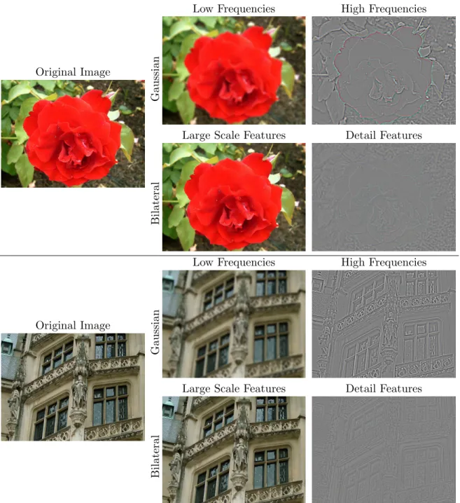
The utility of bilateral filtering goes beyond applications in edge-preserving noise

reduc-tion filtering. The output of the bilateral filter contains smooth regions separated by sharp

edges, which are commonly called the large-scale features. These large-scale features can be

considered a piecewise-constant approximation of the original image. The differences between

the original image and the bilateral filter’s output are the detail features which contain the

textures, as shown in Figure 2.1. The utility of this large-scale/detail decomposition was

orig-inally discussed in terms of High Dynamic Range (HDR) processing by Durand and Dorsey

(2002), where each component was processed separately. More generally, the decomposition

and recomposition of image components is related to earlier work by Peli and Lim (1982),

who used high-pass and low-pass frequency separation of signals in a similar manner.

There have also been many extensions to the bilateral filter. Boomgaard and Weijer (2002)

posed the question of how to improve the robustness of the bilateral filter’s noise-handling

by considering alternate dissimilarity values (Eq. 2.7) that measure photometric differences. The trilateral filter (Choudhury and Tumblin, 2003) takes a different approach to improving

the bilateral filter model by biasing its kernel away from edges and dynamically choosing the

(28)

Original Image

Low Frequencies

Gau

ssian

Large Scale Features

Bilateral

High Frequencies

Detail Features

Original Image

Low Frequencies

Gau

ssian

Large Scale Features

Bilateral

High Frequencies

Detail Features

(29)

functions in the limit. Although the quality of filtering is improved, performance is decreased.

If speed is required, a fast bilateral implementation (O(log r), where r is the kernel radius) is presented by Weiss (2006) that assumes no spatial falloff (i.e.,σh =∞).

To specifically address the reduction of severe shot noise and salt-and-pepper noise,

statistically-motivated rank order filters were introduced. These filters sort the values in

the kernel Ω and use that information to select only certain values to use, such as the median,

minimum, or maximum. The most popular of these is the median filter (Tukey, 1971), which

chooses the median intensity from all intensities in the kernel. This reduces noise, but can

corrupt edges by growing or shrinking them (dilation or erosion) similar to Sigma filtering,

as they are influenced by the kernel’s samples.

The “bilateral median” filter described by Francis and Jager (2003) combines bilateral

filtering and median filtering to reject outliers from the bilateral kernel. Garnett et al. (2005)

used a robust Rank Order Absolute Difference (ROAD) metric to robustly detect if the

bilateral kernel itself is centered on a sample of shot noise. This metric is the sum of the

absolute differences of the n most similar neighboring pixels to the kernel’s center value Is.

The original bilateral filter preserves shot noise because it is considerably different from its

neighbors, but the ROAD metric distinguishes shot noise from actual edges that appear in neighboring pixels.

To demonstrate the effects of many of these standard filters, comparisons are provided in

Figures 2.2 and 2.3. These filters are designed for 2D still images, so their kernels are entirely

spatial. For video noise reduction, however, 3D kernels that utilize temporal information

become possible.

2.3.2 Video Filtering

When processing videos, as opposed to still images, noise filtering can be performed

consid-ering information from adjacent temporal samples to introduce more samples into the kernel

and improve consistency in the filtering from frame-to-frame (temporal coherence). For

in-stance, Dubois and Sabri (1984) perform non-linear temporal noise filtering assisted by optical

(30)

Original Image Gaussian Filter

Sigma Filter Median Filter

Anisotropic Diffusion Filter Bilateral Filter

Figure 2.2: Comparison of existing spatial filtering techniques. The original image exhibits a high noise level in both luminance and chrominance. The Gaussian filter (σ = 5.0) blurs the edges but removes the noise. The Sigma filter (σ = 30) preserves some of the edges but corruption begins to occur at this Ω kernel size (11x11). The 11x11 median filter preserves many eges, but introduces new distortion in blotchy regions. Anisotropic diffusion (50 iter-ations with K = 7) does an excellent job, save some stray pixels in the background. The bilateral filter (σh = 5 and σi = 30) also does an excellent job filtering in a single pass with

(31)

Original Image Gaussian Filter

Sigma Filter Median Filter

Anisotropic Diffusion Filter Bilateral Filter

Figure 2.3: Additional comparison of spatial filtering techniques with a surveillance data source of a stairwell. In very low-light, the original amplified image suffers from very high noise levels. The Gaussian filter (σ = 3.0) blurs the edges, making the scene difficult to interpret. The Sigma filter (σ = 20 with a Ω kernel size = 7x7) does a good job, but is somewhat blotchy. The 5x5 median filter also results in a blotchy image. Anisotropic Diffusion (50 iterations with K = 4) has some trouble reducing the large amount of shot noise, especially on the walls. The bilateral filter (σh = 5 andσi = 15) does the best overall

(32)

temporal filter weighted by the reliability of the displacement estimate. This method requires

well-exposed, easy-to-track video to correctly filter.

Jostschulte et al. (1998) presented a spatio-temporal shot noise filter that first spatially and then temporally filters video while preserving edges that match a template set. A

motion-sensing algorithm is used to vary the amount of temporal filtering. Thus, its filtering can be

considered as a 2D spatial filter augmented by temporally-adjacent samples, thus time and

space are treated differently. Alternatively, “Spatio-Temporal Anisotropic Diffusion” (Lee

and Kang, 1998) uses a three-dimensional kernel to remove video noise, treating temporal and

spatial dimensions similarly. This approach is a 3D variant of the 2D anisotropic diffusion

already discussed in Section 2.3.1.

As opposed to filtering in the local spatio-temporal neighborhood, the NL-means noise

reduction of Buades et al. (2005) searches for matching neighborhoods, which may or may

not be spatially aligned or temporally continuous, to attenuate noise. These neighborhoods

are used to refine the information about the correct underlying values in the original, noisy

neighborhood. In contrast, by finding a statistical mapping of a known video to a set of many

small spatio-temporal training patches “Video Epitomes” (Cheung et al., 2005) allows the

simultaneous enhancement of many similar video regions. This is used for noise reduction in addition to super-resolution and the estimation of dropped video frames.

Video noise filtering is effective because each pixel can incorporate information from many

frames to estimate its true value using images (frames) that are very similar to it. This is

analogous to HDR capture, where each luminance value is combined from a set of registered

images with varying exposures.

2.4 HDR Processing

The real world has a much higher luminance dynamic range than the standard 8-bit sensors and displays in the imaging pipeline, only capable of a 256:1 maximum dynamic range. High

Dynamic Range (HDR) imagery that can represent more realistic dynamic ranges, often

on order of 10,000:1 or 100:000:1, has thus been long recognized as essential for accurately

(33)

There are two problems that quickly become evident working with HDR. First, capture

of HDR imagery is impeded by sensors and digitizing precision, requiring multiple images at

different exposures to properly image all visual elements. Even worse, HDR video capture requires the use of specialized imaging hardware. Another problem is display on 8-bit devices,

requiring a remapping of the image luminances (tone mapping) to match the display’s low

dynamic output range. Thus, HDR processing is a class of computational photography

prob-lem because the correct answers cannot be obtained through a single image or standard image

capture process. Instead, through the combination of multiple images and computation, a

more accurate and useful result is obtained.

2.4.1 HDR Capture

Methods for real-world HDR capture are now considered for both still images and video.

Special consideration is given to the handling of low luminance levels (common in low-light

video) in addition to more typical bright HDR luminance levels. Further low-light imaging

characteristics are addressed in detail in Chapter 4.

Debevec and Malik (1997) developed computational methods for assembling individual

still HDR images from a series of photographs with increasingly long exposure times, using a

common photographic process known as bracketing. The exposure curve of the camera used

to capture these images can be solved for, allowing the determination of a luminance estimate

at each photosite, which is no longer limited by the precision of the source images. This work

relies upon the stillness of the scene over a period of time sufficient to capture each of the

bracketed exposures, making it impractical for video.

Researchers have more recently also constructed prototype HDR video capture systems. Kang et al. (2003) built a system based on a camera that can sequence through different

exposure settings for each frame. Once the images are registered using optical flow, it is

possible to combine exposures to increase the dynamic range. The small number of exposures

combined into each output frame suggests that a high signal-to-noise ratio (SNR) is assumed

for all exposure settings, and therefore, it is designed for well-lit HDR scenes.

(34)

is placed in front of the CCD. The LCD’s per-pixel transparency is varied to modulate the

exposure of image regions based on the previous frame’s luminance. Along with the hardware,

they also discuss a local and global tone mapping approach that addresses temporal coherence issues. Using LCDs implies attenuation of some minimum percentage of the incoming light,

which complicates capturing dark pixels. Nayar and Branzoi (2004) also introduce a variant

to this method using a DLP micromirror array to modulate the exposure, via time-division

multiplexing (like a camera shutter), throughout the image. In theory, such systems could

provide continuous exposure control at each pixel given the additional hardware requirements.

Note that both of these approaches rely on causal filtering to determine the exposure of each

pixel at capture time. If any pixel is over or underexposed because of an incorrect exposure

time, the photosite’s measurement becomes unusable.

Instead of blocking light reaching the sensor, the sensor itself may be modified for HDR

video capture. Acosta-Serafini et al. (2004) describe an HDR camera that selectively resets a

pixel based on a prediction of when it will saturate. Here, the reset interval and the digitized

pixel intensity level combine to form a floating-point intensity value. They primarily focus on

high-speed HDR sensing and do not specifically address low-light capture. Liu and El Gamal

(2003) combine high-speed samples to reduce noise and improve dynamic range by using specific imaging device features such as high-speed non-destructive reads. Their filtering

is based on a combination of linear filters and motion detection at each individual pixel.

Bidermann et al. (2003) describe an HDR high-speed CMOS imaging platform with per-pixel

ADCs and storage, which could use the underlying algorithms of Liu and El Gamal (2003) to

capture HDR in well-lit scenes.

2.4.2 HDR Tone Mappings

Using the discussed HDR capture techniques to create images with dynamic ranges larger than

256:1, the images must then be tone mapped for display while minimizing loss of perceived

detail and contrast.

The tone mapping problem was formalized by Tumblin and Rushmeier (1993) and has

(35)

and spatially varying (Tumblin and Turk, 1999) (Durand and Dorsey, 2002)(Fattal et al.,

2002) tone mappings. By spatially varying the tone mapping, a technique may locally adapt

to maximize displayable contrast. For example, Retinex approaches, such as the multiscale Retinex (Jobson et al., 1997), suggest that a Gaussian-like kernel can be convolved at each

point in the image and subtracted from the original image in log space, resulting in a more

“viewable” version of an HDR still image. The Retinex approach is fast due to it being

non-iterative, but it can generate unwanted edge blurring artifacts because of its underlying

Gaussian nature.

The tone mapper of Durand and Dorsey (2002) presents a similar system, but uses bilateral

filtering to maintain sharp edges and to reduce fringing artifacts. It operates by separating

the large-scale features from the detail features and processes them separately. As shown

in Figure 2.4, this processing is done in the log-luminance domain, which models the detail

features as modulations to the large-scale features (contrast modifications), instead of being

additive. Once the separation has occurred, the large-scale features are attenuated by some

factor k < 1, then recombined into the output. The resulting image then has a reduced dynamic range. The technique works because, after compression, all of the uniform regions

fall within an 8-bit range. The lower magnitude textures are also visible because they are modulating luminances in that displayable range. The results still look plausible because the

contrast ratios are unchanged in smooth regions, only the absolute luminances are modified,

and by Retinex theory (Jobson et al., 1997), the human visual system is not sensitive to

smooth absolute luminance changes over large spatial areas.

Other HDR work includes that of Pattanaik et al. (2000) who present an approach that

mimics the time dependent local adaptation of the human visual system. They also discuss

temporal coherence issues to avoid introducing frame-by-frame tone mapping “flicker” when

processing videos. In “Gradient Domain HDR Compression” (Fattal et al., 2002), the gradient

field of an image is locally attenuated and then reintegrated. It should be noted that they

also describe a method for improving images that already use the display’s full 8-bit dynamic

range. This is the closest problem addressed in the literature to the reverse problem of

(36)

HDR Input ln exp Tone-Mapped_Result

Bilateral *k

+

-Large-Scale

Features

Detail Features

HDR Input Large-Scale Features Detail Features Tone-Mapped Result

Figure 2.4: Illustration of the HDR tone mapping pipeline described by Durand and Dorsey (2002). The result of the bilateral filter, the large-scale features, are attenuated by a factork

while everything else, the detail features, remain unchanged. The tone mapping is performed in the log domain so that the detail features modulate the large-scale features (images shown have been converted to the linear domain for display). Values ofk < 1 cause dynamic range compression (as originally published) while values ofk >1 expand the dynamic range.

By using multiple images, HDR capture and tone mapping create resulting images that

were not otherwise possible to capture. Another approach that combines multiple images is

multispectral fusion. Because these images are now each from a distinctive spectrum, their

fusion creates enhanced results not visible to the human eye.

2.5 Multispectral Fusion Techniques

Multispectral fusion involves the depiction of multiple, potentially non-visible, spectral bands

as a visible image. The goal can be to communicate information from all sources, or to

augment a poor quality signal in one band with a higher quality one (such as augmenting noisy

night-vision video with heat-detection imagery). In this section, two classic multispectral

applications are summarized: remote sensing (aerial and satellite imagery) and night-vision.

(37)

a neural network to create false-color (pseudo-color) images from a learned opponent-color

importance model. Many other false-color fusion models have been suggested in the remote

sensing community. A summary of popular techniques is provided by Pohl and Genderen (1998). Another common fusion approach is to combine pixel intensities across spatial scales

using multiresolution Laplacian or wavelet pyramid decompositions, as in (Toet, 1990) and

(Li et al., 1994). Also, physically-based models that incorporate more than per-pixel image

processing have also been suggested (Nandhakumar and Aggarwal, 1997).

Therrien et al. (1997) introduce a method to decompose visible and IR sources into their

respective high and low frequencies, and processes them in a decomposition/recomposition

framework inspired by Peli and Lim (1982). A non-linear mapping is applied to each set

of spectral bands to fuse them into the result. Therrien et al. (1997) address normalizing

luminance responses between spectra to overcome differences in surface reflectivity between

bands. These normalized luminances are mapped to a new space defined by a Sammon

mapping (Sammon, 1969). Issues regarding the temporal coherence of such a mapping in

video are not mentioned.

IR colorization algorithms, such as those by Welsh (2002) and Toet (2005), attempt to

learn a mapping from IR to natural chrominance to construct a plausible colorized output. For that reason, colorization can be considered a class of fusion that estimates chrominance

based on image priors from IR footage. However, acquiring a prior and performing accurate

matching from prior to IR is often difficult and does not guarantee temporal coherence for

video processing.

2.6 Computational Photography

Having considered combining elements from multiple spectra together (often imaged

simulta-neously), we next consider combining exposures taken with the same imager, but at different times. This allows for existing imagers, such as digital cameras and camcorders, to achieve

enhanced results with the assistance of computational methods.

Therefore, I now present techniques that are typically labeled as computational

(38)

to create an optimal composite image. Specifically, multiple images are used as input, and a

still image is the result. These combination techniques draw on the wealth of algorithms and

techniques that have already been discussed in this chapter.

“Image Stacks” (Cohen et al., 2003) considered the idea of using multiple temporally

adjacent frames to enhance knowledge about a pixel’s true or desired value. Multiple images

are registered and then each pixel of the output image is computed as a function of its temporal

neighbors. “Image Stacks” includes methods for automatically selecting and combining image

regions using compositing and min, max, median, and temporal low-pass filtering. An α -blended “over” compositing (Porter and Duff, 1984) (Eq. 2.8) is also used to illustrate the

passage of time by compositing so that recent motions occlude past motions:

Over =α·F oreground+ (1−α)·Background. (2.8)

The concept of combining sequential frames of motion together can be traced back to

the stroboscopic multiple exposure photographs of Harold Edgerton (Edgerton and Killian,

1979) and the motion studies of Muybridge (Muybridge, 1955) and Marey (Braun, 1995),

all performed using traditional film capture. The combination of images to create motion

studies was also addressed by Freeman and Zhang (2003) with the use of stereo depth data

to influence each pixel’s compositing order.

As an extension to “Video Stacks”, “Interactive Digital Photomontage” (Agarwala et al.,

2004) allows the user to choose individual parts of a few images through a simple drawing

interface to quickly specify the best composite image. This fusion is accomplished using both graph-cut (Kwatra et al., 2003) and gradient domain algorithms (see below).

“Space-Time Scene Manifolds” (Wexler and Simakov, 2005) combined the concept of using

spatio-temporal volumes (Section 2.2) with a similar goal of combining multiple sequential

video frames captured with a non-static camera. The resulting optimized non-planar cuts are

chosen to maximize the visual information in the resulting cut image while simultaneously

mosaicing the constituent video frames.

The seamless integration of scene elements from multiple images has been explored in

(39)

solvers have already been mentioned in the context of HDR tone mapping (Section 2.4.2).

Techniques such as Poisson Image Editing (Perez et al., 2003), and day/night fusion (Raskar

et al., 2004) generate gradient fields that contain visual elements from multiple images. The ratio-image work of Liu et al. (2001) transfers illumination between multiple images

with the assistance of known illumination priors. The capture of these priors requires images

taken in controlled lighting environments, which are suited for still images, but not for video.

New variants of the bilateral filter, discussed in Section 2.3.1, have been developed for use

in computational photography. The “joint bilateral filter” uses a second image as the source

of comparison for edge identification, thus transferring its edges to the original image. This

filter was used by Petschnigg et al. (2004) and by Eisemann and Durand (2004) (who refer

to it as “the cross bilateral filter”). Both of these papers consider the problem of combining

the qualities of an image captured with the use of a flash with the “look” of a noisy image

captured under ambient illumination. A joint bilateral filter is created by changing Equation

2.7 to instead perform its photometric comparisons in a second image, indicated asI0:

D(p, s)≡I_p0 −I_s0. (2.9)

The extent of noise removal depends on how well exposed a given region is in the flash

image. These papers also address flash shadows, which introduce visible edge differences

between the sources. These flash shadows resemble some of the differences seen between

RGB and IR spectra mentioned in Section 2.5.

These approaches are all designed to output a single image as a function of its input frames. In the final section, computational video techniques that result in video outputs are

considered.

2.7 Computational Video

Computational video is a more recent field than computational photography, so its seminal

literature is not yet established. In this dissertation, computational video involves processing

(40)

This is accomplished using techniques enabled by modern computational power and the

si-multaneous processing of many frames enabled by the low cost of storage. One type of

computational video is the temporal resampling of a video to change its duration. Com-putational video techniques are thus allowed to warp both space and time, compressing or

extending the video’s duration and intermixing frames.

2.7.1 Video Summarization

Temporal resampling is commonly used for multimedia summarization. Early work in Video

Skimming (Smith and Kanade, 1997) looked for short, representative video segments that,

when pieced together, could tell the story of the video in a reduced period of time. Segments were chosen based on characteristics including scene change detection, camera motion, object

recognition, and audio. The documentary films they targeted had distinct scene changes

providing the algorithms additional hints. An alternate summarization approach proposed

by Hua et al. (2003) searched for video segments that contain scene and camera motion

between shot boundaries and combined them to match the rhythm of an audio source to

create music videos.

Using similar documentary films to (Smith and Kanade, 1997) and standard,

uniformly-sampled summarization (fast-forward), Wildemuth et al. (2003) explored how fast videos can

be played back while remaining coherent to the viewer. The result was that showing 1 out

of every 64 frames typically allowed the viewer to comprehend most of the content. Note

that in addition to documentary-style video sources, summarization can also be applied to

static-camera, time-lapse sources. In particular, time-lapse has been shown to have many

applications for viewing slowly changing processes. Time-lapse techniques are regularly used in fields as varied as biological microscopy (Riddle, 1979) and cinematic effects (Kinsman,

2006).

“Video Summarization By Curve Simplification” (DeMenthon et al., 1998) presents an

algorithm to choose a non-uniform temporal sampling based upon simplification of tracked

motion-path curves. These motion curves can be considered a subset of all motion activity

(41)

curve-fitting algorithm (Douglas and Peucker, 1973). Note that slower, but optimal, dynamic

programming-based curve-fitting solutions (Perez and Vidal, 1994) are possible.

In “Video Summarization Using MPEG-7 Motion Activity and Audio Descriptors” (Di-vakaran et al., 2003), short video sub-clips identified as containing significant motion are

played at real-time speeds and assembled into a shorter video. The combined duration of

these essential sub-clips forms the lower bound of the output video’s duration. Longer videos

are constructed by padding the result with less interesting frames.

Rav-Acha et al. (2006) summarize long videos by allowing events to occur without the

strict chronological ordering of the source footage, thus events may overlap. The events are

identified and then combined in a manner determined via a spatio-temporal Markov random

field optimization and simulated annealing.

2.7.2 Temporal Resampling and Compositing

Computational video considers a wider range of temporal resamplings and frame

combina-tions. For instance, a class of operations exist that extend the length of videos by repeating

segments. “Video Textures” (Sch¨odl et al., 2000) looks for transitions within a video that are

least noticeable in an attempt to indefinitely extend its playing time. A dynamic programming

solver is used along with a pairwise error metric to evaluate potential jumps.

Other approaches have also attempted to warp time, both globally (full frame) and locally

(region-by-region). “Flow-Based Video Synthesis and Editing” (Bhat et al., 2004) rearranges

repeating patterns of natural phenomena, such as waterfalls, that have reoccurring flow

char-acteristics, to extend their play time. “Evolving Time Fronts” (Rav-Acha et al., 2005a) plays

videos with differing speeds in multiple image regions for the effect of altering their outcomes or for artistic effects. “Dynamosaics” (Rav-Acha et al., 2005b) carries this idea further by

improving the blending between regions with graph-cuts (Boykov et al., 1999). “Panoramic

Video Textures” (Agarwala et al., 2005) also finds frame-to-frame jumps within non-static

camera videos to create panoramas.

Videos can also be processed to alter their component visual elements. “Motion

(42)

changing the underlying temporal sampling, thus increasing apparent object velocity.

Al-ternatively, “Space-Time Super-Resolution” (Shectman et al., 2005) creates a composite of

multiple videos using their relative frame rates and spatial positions to maximize spatial and temporal information while reducing overall aliasing.

As a parallel to these computational video methods, user-assisted, temporally-aware video

compositing algorithms have also been developed. “Video Matting of Complex Scenes”

(Chuang et al., 2002) approaches the problem using Bayesian methods. “Interactive Video

Cutout” (Wang et al., 2005) combines compositing with spline-based, non-planar

spatio-temporal volume cuts in its interface for extracting foreground elements. In this interface,

the user can specify hints to the alpha compositing engine across multiple frames by painting

directly onto the cut plane. The VideoShop project (Wang et al., 2007) composites

multi-frame visual elements from video clips together in the gradient domain through the use of a

3D multigrid Poisson solver.

2.8 Summary

A wide range of literature related to computational video and its foundations was reviewed to

act as a background for the techniques and applications presented throughout the remainder of

this dissertation. The common element in all of these works is the visualization, combination,

and enhancement of still images and videos to create improved outputs by utilizing all the

information in the source material. As a first step to building efficient computational video

tools, a framework is now presented for working with a new class of spatio-temporal volumes

(43)

CHAPTER 3

SPATIO-TEMPORAL VIDEO

PROCESSING

In this chapter, I explore approaches to computational video where videos are abstracted as

spatio-temporal volumes. Computational video often relies on using nearby spatial and

tem-poral samples in order to enhance the underlying video. Likewise, spatio-temtem-poral volumes

provide a representation for accessing and organizing these samples. Furthermore, I extend

spatio-temporal volumes to include sheared volumes that spatially align frames to bring

to-gether important scene elements into a common spatio-temporal neighborhood. This shearing

can be done in relation to the background to stabilize a moving camera, or in relation to a

moving object to stabilize its motion.

Frequently, shears are not meant to be permanent. Therefore it is desirable after

process-ing that the original camera and object motions be restored. Thus, modifications made to

these sheared volumes must be applied to the source data and are formulated as mapping

functions, thus making the shearvirtual. Furthermore, there are significant performance

is-sues involved in manipulating and visualizing uncompressed spatio-temporal video volumes in sheared and un-sheared states. To handle these issues, an efficient graph-based processing

framework called Proscenium is introduced to encapsulate and abstract away the details of

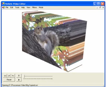
such processing. Finally, as a proof-of-concept, a simple video editor is developed that

visual-izes, edits, and filters in a manner that leverages the capabilities of spatio-temporal volumes

(Figure 3.1).

The chapter begins with discussions of previous spatio-temporal volumes and then an

overview of the new shearing extension. Then, spatio-temporal video processing with