Lee_unc_0153D_16429.pdf

(1)

DYNAMICS AND SOCIAL CLUSTERING ON COEVOLVING NETWORKS

Hsuan-Wei Lee

A dissertation submitted to the faculty at the University of North Carolina at Chapel Hill in partial fulfillment of the requirements for the degree of Doctor of Philosophy in the Department of

Mathematics in the College of Arts and Sciences.

Chapel Hill 2016

(2)

(3)

ABSTRACT

Hsuan-Wei Lee: Dynamics and Social Clustering on Coevolving Networks

(Under the direction of Peter J. Mucha)

Complex networks oﬀer a powerful conceptual framework for the description and analysis of many real world systems. Many processes have been formed into networks in the area of random graphs, and the dynamics of networks have been studied. These two mechanisms combined creates an adaptive or coevolving network – a network whose edges change adaptively with respect to its states, bringing a dynamical interaction between the state of nodes and the topology of the network.

We study three binary-state dynamics in the context of opinion formation, disease propagation and evolutionary games of networks. We try to understand how the network structure affects the status of individuals, and how the behavior of individuals, in turn, affects the overall network structure. We focus our investigation on social clustering, since this is one of the central properties of social networks, arising due to the ubiquitous tendency among individuals to connect to friends of a friend, and can significantly impact a coevolving network system. Introducing rewiring models with transitivity reinforcement, we investigate how the mechanism affects network dynamics and the clustering structure of the networks.

(4)

(5)

ACKNOWLEDGEMENTS

I would like to express my sincere gratitude to my advisor Peter J. Mucha for his support, encouragement, and patience. His guidance helped me in all the time of research and writing of this thesis. He gave me time to learn and the freedom to choose the topics I love and is always very helpful when I need his help and advice. I could not have imagined having a better advisor and mentor for my Ph.D. study.

Besides my advisor, I would like to thank my collaborator and mentor Nishant Malik greatly. Nishant was a postdoc fellow with Peter, so again I want to thank Peter for steering our eﬀorts in this direction. Nishant had helped me through the toughest time of my early research, spent a lot of time on discussing mathematical ideas and helping me writing better codes. My sincere thanks also go to my collaborators Feng (Bill) Shi and Huan-Kai Tseng. Bill was also a graduate student of Peter’s, and we collaborated on the work provided in Chapter 2 and Chapter 3. He always gives me great insights and is always very kind and supportive. Huan-Kai is my good friend and also a political scientist. Although I didn’t put our work in my thesis, his help of applying for the work in Chapter 4 to world trade broadens the scope of my research to the real world. I thank my fellow Mucha group-mates Dane Taylor, Saray Shai, Clara Granell, Simi Wang, Natalie Stanley and Samuel Heroy for all the fun we have had in the last few years. They gave me great feedbacks to my work and talks, and also from them, I learned a lot in the diﬀerent fields of Complex Systems.

Final thanks to the members of my thesis committee David Adalsteinsson, Shankar Bhamidi, Greg Forest, and Jingfang Huang for their insightful comments, useful discussions, and encouragement in the preparation of this thesis.

(6)

TABLE OF CONTENTS

LIST OF FIGURES . . . ix

CHAPTER 1: INTRODUCTION . . . 1

1.1 Networks Overview . . . 1

1.2 Networks with Complex Structural Properties . . . 2

1.3 Network Dynamics and Coevolving Networks . . . 5

1.4 Analytical Methods . . . 6

1.5 Overview of Thesis . . . 9

CHAPTER 2: VOTER MODEL AND SOCIAL CLUSTERING ON COMPLEX NETWORKS . . . 11

2.1 Background Information . . . 11

2.2 Model Description . . . 13

2.3 Semi-analytical Methods . . . 15

2.4 Numerical Experimentation and Discussion . . . 19

2.4.1 Consensus States of the Networks . . . 19

2.4.2 Clustering Coeﬃcients . . . 20

2.4.3 Degree Distribution . . . 21

2.4.4 Qualitative Exploration . . . 23

2.4.5 Semi-analytical Approximation . . . 25

2.5 Conclusion . . . 26

CHAPTER 3: SIS MODEL AND SOCIAL CLUSTERING ON COMPLEX NET-WORKS . . . 29

(7)

3.4 Numerical Experimentation . . . 33

3.4.1 Exploration of the Parameter Space . . . 34

3.4.2 Network Dynamics and the Eﬀect of⌘ . . . 34

3.4.4 Clustering Coeﬃcient . . . 40

3.4.5 Disease Prevalence . . . 40

3.4.6 Bifurcation Analysis . . . 44

CHAPTER 4: EVOLUTIONARY GAMES ON COMPLEX NETWORKS . . . . 50

4.4.2 Final Level of Cooperation . . . 65

4.4.3 Network Dynamics . . . 67

4.4.5 Exploration of the Initial Fraction of Defectors,⇢ . . . 72

4.5 Discussion . . . 74

CHAPTER 5: EVOLUTIONARY GAMES ON COMPLEX NETWORKS – A VARI-ATION MODEL . . . 79

5.3.2 Final Level of Cooperation . . . 85

(8)

5.3.5 Exploration of the Initial Fraction of Defectors,⇢ . . . 92

CHAPTER 6: LINK-BASED EVOLUTIONARY GAMES ON COMPLEX NET-WORKS . . . 96

6.2.1 Mean Field Approximation . . . 99

6.2.2 Pair Approximation . . . 100

6.3 Numerical Results and Discussion . . . 101

CHAPTER 7: SUMMARY . . . 104

APPENDIX A: VOTER MODEL AND SOCIAL CLUSTERING ON COMPLEX NETWORKS . . . 107

A.1 Evolution of Clustering in the model . . . 107

A.2 Degree Distribution . . . 108

A.3 Transitions . . . 109

(9)

LIST OF FIGURES

2.1 Illustration of the clustering reinforcement mechanism. At each time step, a discordant edge is picked. There is probability↵ for one node rewires to its neighbor’s neighbor and closes a triangle. In this figure, white nodes are with opinion 0 and gray nodes are with opinion 1. A discordant edgeXY is picked and nodeY dismissesX and it rewires to its distance two neighbor W. . . 11 2.2 Suppose the center is a node with opinion 0. The following are illustrations of the

center passively rewired by diﬀerent distance two neighbors: (a) 0 rewires to node X, a class of Sk,m, (b)1 rewires to node Y, a class ofSk,m, (c) 0 rewires to node Z,

a class ofSk 1,m and (d)1 rewires to node W, a class of Sk 1,m 1. The case of the

center with opinion1 is similar. . . 14 2.3 (a) Levels of ⇢, the fraction of nodes holding minority opinions in the consensus states

with diﬀerent combinations of ↵ and . In the hegemonic consensus state region, the minority opinion fraction is close to 0. However, in the segregated consensus state region, the minority opinion fraction is close to 0.5. Note that when increases, the region of the hegemonic consensus shrinks. (b) Levels ofs1, the size of the largest

connected component in the consensus state with different combinations of ↵ and . In the hegemonic consensus state region, the largest connected component in the consensus state is close to 1, the original size of the network. On the other hand, in the segregated consensus state region, the largest connected component in the consensus state is close to 0.5, half of the original size of the network. . . 16 2.4 (a) Evolution of clustering coefficients with different values of with ↵= 1. Circles

are the clustering coefficients in the consensus states. (b) The clustering coefficients with different values of with↵ = 1in the consensus states at timetf. Circles denote

the simulation results, and the line denotes the theoretical estimation. . . 17 2.5 Initial and final degree distributions in the consensus state with diﬀerent values of

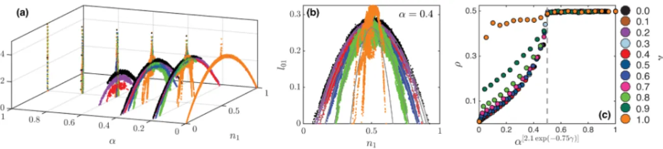
↵ and . We start with Erdős-Rényi networks with mean degreehki= 4, which has a Poisson distribution, highlighted by thick gray bands in each subfigure. We see a various level of deviation from the initial degree distribution as↵ and change. . . . 18 2.6 (a) The dynamics of the clustering reinforcement model in the phase space of l01 and

n1 with diﬀerent values of ↵ and . Note that the dynamics forms arches when ↵

is small, and as↵ increases, the size of the arch shrinks. When ↵= 0.8 and↵= 1, there are no such arches formed. Fix↵ = 0.4, the dynamics of the model plotted as l01 versusn1. The width of the arches is squeezed as we increase , and when = 1,

the arch is destroyed. (c) Levels of⇢, the fraction of nodes holing minority opinions in the consensus states versus ↵. Here we transformed ↵ into↵2.1 exp( 0.75 ). Note that this transformation forces all the data for <0.8 collapses onto one universal line. Moreover, there is a clear transition in when↵2.1 exp( 0.75 )= 0.5. . . 20 2.7 Comparison between Approximate Master Equation (AME) and simulations for

(10)

2.8 Comparison between numerical simulations and the semi-analytical solution by Ap-proximate Master Equation (AME) at↵= 0.4. Diﬀerent colors represents diﬀerent values of , the color scheme used here is the same as in Figure 2.4 and Figure 2.5 above. . . 22

3.1 Illustration of rewiring to neighbors’s neighbor. Before the rewiring, nodeXis of class Sk,l (the left subfigure). Suppose a discordant edge Y Z is picked, with probability ⌘, Y would actively dismiss its infected neighbor and rewire to its neighbors’s neighbor X. Then nodeX becomes of class Sk+1,l (the right subfigure). . . 24

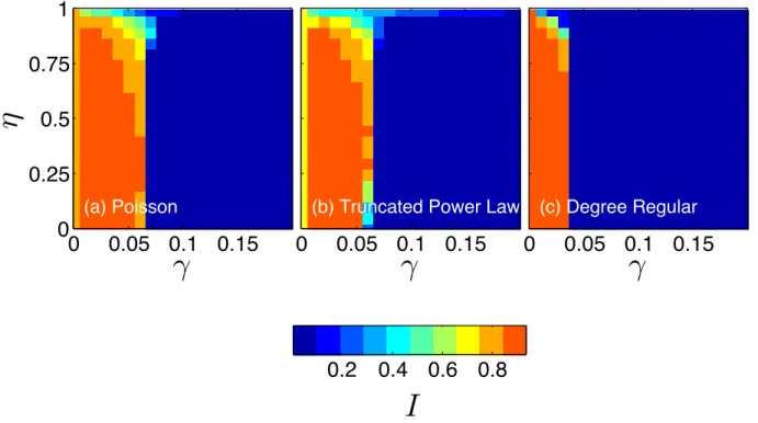
3.2 Phase plots in parameter space ( , ⌘) for the disease prevalenceI on networks with an initial (a) Poisson, (b) truncated power law, and (c) degree regular degree distribution. Other parameters are = 0.04, ↵ = 0.005 and ✏ = 0.1. We choose t = 10,000, when most of the networks reach their stationary states. The disease prevalence I is averaged over 30 simulations in all cases. . . 28

3.3 Disease prevalenceI against time ton networks with mean degreehki= 2but with diﬀerent initial degree distributions (pP_k (Poisson): blue, pT P L_k (truncated power law): magenta, and pDR

k (degree regular): red). Dots correspond to the mean computed over 1,000 simulations and lines are the semi-analytical approximations. Parameters are = 0.04, = 0.04,↵= 0.005 and ✏= 0.1 in all cases. The⌘ here are: (a) ⌘= 0, (b)⌘= 0.2, (c) ⌘= 0.4, (d)⌘ = 0.6. . . 29

3.4 (a) Degree distribution and (b) degree distribution of S andI nodes on networks with mean degreehk_i= 2 on log-log scale but with diﬀerent initial degree distributions (pP_k (Poisson): blue,pT P L_k (truncated power law): magenta, andpDR_k (degree regular): red). Dots correspond to the mean computed over 200 simulations. Solid lines in (a) are the semi-analytical approximation of total degree, dashed lines and dotted lines in (b) are the semi-analytical approximation of degree distribution ofS and I, respectively. Parameters are = 0.04, = 0.04,↵= 0.005,✏= 0.1 and ⌘= 0.4. . . . 31

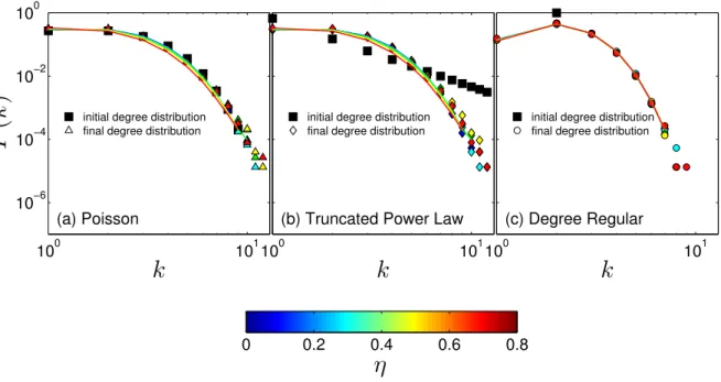
3.5 Degree distribution with mean degree hki= 2on log-log scale on networks with an initial (a) Poisson, (b) truncated power law, and (c) degree regular degree distribution. We choose ⌘ = 0,0.2,0.4,0.6, and 0.8. Other parameters chosen are = 0.04, = 0.04,↵ = 0.005, and✏= 0.1. We sett= 5,000, all networks reach their stationary states at this time. Squares in each subplot are the initial degree distributions. Dots correspond to the mean computed over 200 simulations. Lines are the semi-analytical approximation of the stationary state degree distributions. . . 32

3.6 (a) Clustering coeﬃcient C versus time t on networks with the same mean degree

hki = 2 initial Poisson degree distributions. The parameters of the system are = 0.04, = 0.04,↵= 0.005, and ✏= 0.1.Dots correspond to the mean computed over 30 simulations. Different chosen values of⌘are shown in the figure. (b) Clustering coefficient C att= 5,000versus⌘ on networks with the same mean degreehki= 2 but different initial degree distributions (pP_k (Poisson): blue,pT P L_k (truncated power law): magenta, andpDR

(11)

3.7 Disease prevalence I against timet on networks with the same mean degree_hk_i= 2

initial Poisson degree distribution. The parameters of the system are = 0.04, = 0.04,↵ = 0.005, and ✏ = 0.1. Dots correspond to the mean computed over 1,000 simulations and the lines are the semi-analytical approximation. Diﬀerent chosen values of⌘ are shown in the figure. . . 35

3.8 Disease prevalence I against timetuntil t= 107 _{in the case} _⌘_{= 1} _{on networks with}

mean degreehki= 2initial Poisson degree distributions. (a) Dots are sampled every t

= 1,000 correspond to the mean computed over 30 simulations. (b) The curve fitting on a log log plot of the data. We can see the data becomes a straight line and this suggests the data has a power law decay. . . 36

3.9 (a) Disease prevalenceI versus⌘ at time t= 10,000 on networks with the same mean

degree hki = 2 but diﬀerent initial degree distributions (pP_k (Poisson): blue, pT P L_k (truncated power law): magenta, andpDR_k (degree regular): red). (b)tf versus⌘ on

networks with the same mean degreehk_i= 2initial degree regular degree distribution.

Dots correspond to the mean computed over 30 simulations and the lines are the semi-analytical approximations. . . 37

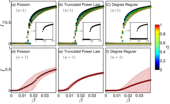
3.10 Bifurcation diagrams of the disease prevalence I versus ⌘ on networks with an initial (a) and (d): Poisson, (b) and (e): truncated power law, and (c) and (f): degree regular degree distribution. In (a), (b) and (c), we plot all the simulation results of 30 experiments. In (d), (e) and (f), dots and the error bar are the mean and standard deviation over 30 Monte Carlo simulations. The first row are the cases⌘<1

and the second row are the cases⌘= 1. We vary the values of and⌘. The other parameters of the system are = 0.02, and ↵= 0.005. We run simulations for each

value ✏= 0.001,0.01,0.05,0.99, and,0.999. We set t= 10,000, all networks with ⌘ not close to 1 reach their stationary states at this time. . . 38

3.11 Bifurcation diagrams of the disease prevalence I versus ⌘ on networks with an initial (a) Poisson, (b) truncated power law, and (c) degree regular degree distri-bution. Lines are the predictions of our semi-analytical approach and dots are the outcome of 30 Monte Carlo simulations. We run simulations for each value ✏= 0.001,0.01,0.2,0.4,0.6,0.8,0.99, and, 0.999and plot them with diﬀerent colors.

We sett= 10,000, all networks with⌘ not close to 1 reach their stationary states at this time. . . 39

(12)

4.2 Illustration of the strategy updating process. Pick a discordant edgeXY. Suppose

nodeX is of stateC and nodeY is of stateD. Then with probability w, the strategy

updating process happens. Node X andY would compare their utility and the node

with lower utility would change its strategy with probability according to the Fermi functions. Supposeu= 0.5, then nodeX has 1 unit of utility and node Y has 4 units

of utility. By the Fermi function, (sX sY) = _1+exp[_↵_(P1_X _P_Y_)] = _{1+exp[30(1 4)]}1 ⇡1,

that is nodeX has a probability close to 1 to imitate nodeY’s state. . . 44

4.3 Visualization of the partner switching model soon before fission occurs, forN = 1,000

nodes,M = 5,000 edges, cost-to-benefit ratiou= 0.5, strategy updating probability w= 0.1, and initial fraction of defectors ⇢= 0.5. Colors correspond to the two states

of node; blue: cooperative and red: defective. . . 46

4.4 Illustration of transitions to/from the Ck,l and Dk,l sets in the AME. For each set,

only parts of its neighbors are shown here, and the classes of sets are shown next to the corresponding compartments. . . 48

4.5 Illustration of active rewiring. Before the rewiring, node X is of classCk,l. Suppose

one ofX’s discordant edge is picked, and X actively dismisses its defective neighbor,

rewiring to a random node in the network. If nodeX rewires to a node of stateC,

then node X becomes of classCk+1,l. We recall that only C’s actively rewire in the

present model. . . 50

4.6 Illustration of passive rewiring. Before the rewiring, node X is of classCk,l. Suppose

in the rewiring process, nodeX is passively rewired by a random node in the network.

Then node X becomes of classCk+1,l. We recall that only C’s actively rewire in the

present model. . . 51

4.7 Simulation results of the final fraction of cooperators with diﬀerent combinations ofu

andw. For bothu andw axes, we pick the step to be 0.05 and plot the fraction of

cooperators in the stationary states in simulations. We take the mean of 50 simulations of each parameter set here. . . 52

4.8 Fraction of cooperators versus cost-to-benefit ratio uwith diﬀerent strategy updating

rates w in stationary states. Markers are the averages of 1,000 simulations results,

dotted lines are the semi-analytical results of pair approximation (PA), and the dashed lines are the semi-analytical results of approximate master equations (AMEs). The PA results are diﬀerent from the ones shown in [46], but we have confirmed the accuracy of our results in personal communication with the authors of that paper. . . 53

4.9 Fraction of cooperators versus w with diﬀerent cost-to-benefit ratio u values in

(13)

4.10 Evolution of five fundamental quantities versus time t when u = 0.5 and w = 0.1.

We plotC (blue), D (red),CC (green), CD (magenta), andDD (black) ratios and compare these with two semi-analytical approximations. Markers are the averages of 50 simulations results, dotted lines are the semi-analytical results of pair approximation (PA), and the dashed lines are the semi-analytical results of approximate master equations (AMEs). PA dynamics stop aroundt= 10, and it gives bad estimations.

On the other hand, AME provides better estimations of the simulation results. . . . 56

4.11 Evolution of five fundamental quantities versus time t in diﬀerent parameter sets, upper left: u = 0.2, w = 0.1, upper right: u = 0.2, w = 0.3, lower left: u = 0.5,

w = 0.1, and lower right: u = 0.5, w = 0.3. We plot C (blue), D (red), CC (green),CD(magenta),DD(black) ratios and compare these with our semi-analytical approximations. Markers are the averages of 50 simulations results and the lines are the semi-analytical results of approximate master equations (AMEs). AME provides qualitatively good estimations of the simulation results. . . 57

4.12 Degree distribution in the stationary states in diﬀerent parameter sets, upper left: u= 0.2, w= 0.1, upper right: u = 0.2, w= 0.3, lower left: u = 0.5,w = 0.1, and

lower right: u= 0.5, w= 0.3. Bars are the averages of 50 simulations results and the

lines are the semi-analytical results of approximate master equations (AMEs). AME provides qualitatively good estimations of the simulation results. Blue bars and lines are degrees of cooperative nodes, and red bars and lines are degrees of defective nodes. 59

4.13 Fraction of cooperators versus ⇢ withw= 0.1 in stationary states. Diﬀerent

cost-to-benefit ratiou: 0, 0.1, ..., 1 are chosen. Markers are the averages of 50 simulations results and the dashed lines are the semi-analytical results of approximate master equations (AMEs). . . 60

4.14 Simulation results of the final fraction of CC links with diﬀerent combinations ofu andw. For bothu andw axes, we pick the step to be 0.05 and plot the fraction of cooperators in the stationary states in simulations. We take the mean of 50 simulations of each parameter set here. . . 61

4.15 Simulation results of the final fraction of CC links with diﬀerent combinations ofu andw. For bothu andw axes, we pick the step to be 0.05 and plot the fraction of cooperators in the stationary states in simulations. We take the mean of 50 simulations of each parameter set here. . . 62

5.1 Visualization of the second partner switching model in the stationary state, for N = 1,000 nodes,M = 5,000 edges, cost-to-benefit ratiou= 0.5, strategy updating

probability w= 0.1, and initial fraction of defectors ⇢ = 0.5. Colors correspond to

(14)

5.2 Visualization of the second partner switching model in the stationary state, for N = 1,000nodes, M = 5,000 edges, cost-to-benefit ratio u= 1, strategy updating

probabilityw= 0.5, and initial fraction of defectors ⇢= 0.5. Colors correspond to the

two states of node; blue: cooperative and red: defective. In this case, onlyD nodes exist in the network, and all the edges are DDedges. . . 67

5.3 Simulation results of the final fraction of cooperators with diﬀerent combinations of cost-to-benefit ratio u and strategy updating probabilityw. For both uand w axes, we pick the step to be 0.05 and plot the fraction of cooperators in the stationary states in simulations. We take the mean of 50 simulations of each parameter set here. 69

5.4 Simulation results of the final fraction of CC links with diﬀerent combinations of cost-to-benefit ratio u and strategy updating probabilityw. For both uand w axes, we pick the step to be 0.05 and plot the fraction of cooperators in the stationary states in simulations. We take the mean of 50 simulations of each parameter set here. 70

5.5 Fraction of cooperators versus cost-to-benefit ratio uwith diﬀerent strategy updating probabilitywvalues in stationary states. Markers are the averages of 1,000 simulations results, dotted lines are the semi-analytical results of pair approximation (PA), and the dashed lines are the semi-analytical results of approximate master equations (AMEs). 71

5.6 Fraction of cooperators versus strategy updating probability w with diﬀerent cost-to-benefit ratio u values in stationary states. Markers are the averages of 1,000 simulations results, dotted lines are the semi-analytical results of pair approximation (PA), and the dashed lines are the semi-analytical results of approximate master

equations (AMEs). . . 72

5.7 Evolution of five fundamental quantities versus time t when cost-to-benefit ratio u= 1and strategy updating probability w= 0.05. We plotC (blue),D (red),CC (green),CD(magenta),DD(black) ratios and compare these with two semi-analytical approximations. Markers are the averages of 50 simulations results, dotted lines are the semi-analytical results of pair approximation (PA), and the dashed lines are the semi-analytical results of approximate master equations (AMEs). The dynamic stops

evolving when there are noCD andDD edges, which happens aroundt= 220. PA

dynamics stop around t= 10, and it gives bad estimations. On the other hand, the

AME method provides better estimations of the simulation results. . . 74

5.8 Evolution of five fundamental quantities versus time t in diﬀerent parameter sets, upper left: u = 0.2, w = 0.1, upper right: u = 0.2, w = 0.3, lower left: u = 0.5,

(15)

5.9 Degree distribution in the stationary states in diﬀerent parameter sets, upper left: u= 0.2, w= 0.1, upper right: u = 0.2, w= 0.3, lower left: u = 0.5,w = 0.1, and

lower right: u = 0.5, w = 0.3. Bars are the averages of 50 simulations results and

the lines are the semi-analytical results of the approximate master equations (AMEs). AME provides qualitatively good estimations of the simulation results. Blue bars and lines are degrees of cooperative nodes, and red bars and lines are degrees of defective nodes. . . 76

5.10 Fraction of cooperators versus the initial fraction of defectors⇢with strategy updating

probabilityw= 0.1 in stationary states. Diﬀerent cost-to-benefit ratio u: 0, 0.1, ..., 1 are chosen. Markers are the averages of 50 simulations results and the dashed lines are the semi-analytical results of approximate master equations (AMEs). . . 77

5.11 Fraction of cooperators versus the initial fraction of defectors ⇢ with cost-to-benefit

ratiou= 0.2 in stationary states. Diﬀerent w: 0, 0.1, ..., 1 are chosen. Markers are the averages of 50 simulations results and the dashed lines are the semi-analytical results of approximate master equations (AMEs). . . 78

6.1 Visual depiction of the available information maintained in three diﬀerent levels of analytical approximations — mean field (MF), pair approximation (PA), and approximate master equation (AME) —, in link-based dynamical evolutionary games in a network setting. . . 80

6.2 Fraction of cooperators versus cost-to-benefit ratio u with diﬀerent w values in stationary states. Markers are the averages of 100 simulations results and the dashed lines are the semi-analytical results of mean field (MF) approximation (note that all 4 dashed lines forw <1 combine under the black dashed line at the value1). . . 84

6.3 Fraction of cooperators versus cost-to-benefit ratio u with diﬀerent w values in stationary states. Markers are the averages of 100 simulations results and the dashed lines are the semi-analytical results of pair approximation (PA). . . 84

A.1 Values of the parameterb1 in Section 2.4.3 . . . 89

A.2 In this figure we show thatc1/c2⇠↵2.1 exp( 0.75 ) for↵<↵c( ), where ↵c( )is the solution of↵2.1 exp( 0.75 )_{= 0}_.₅_{. The transition point is emphasized by grey dashed line.} _c

(16)

CHAPTER 1 Introduction

1.1 Networks Overview

We are surrounded by systems that are extremely complicated. The emergence of network science is a brilliant demonstration that interdisciplinary science can take up the challenge of studying such systems [9, 110]. These systems are collectively called complex systems, capturing the fact that it is diﬃcult to derive their collective behavior from a knowledge of the system’s components. Network science deals with complexity by summarizing complex systems as components and capturing the interplay between them. Despite or even perhaps because of such simplifications, informative discoveries can and have been made. A network based mathematical and statistical approach is extremely desirable for such endeavors as it is a formalism allowing one to couple microscopic and macroscopic dynamics. The following is a sample of some of the applications in which network science are becoming increasingly significant.

Biological processes are often represented in the form of graphs or networks, and a biological network is any network that applies to biological systems [3, 12, 78]. A biological system could be represented in a framework of networks consisting of a set of nodes representing biological entries and edges denoting relationships between pairs of nodes. Biological networks provide a mathematical model of connections found in ecological, evolutionary, and physiological studies, such as protein-protein interaction networks, metabolic pathways, gene regulatory networks, cell signaling networks, neural networks, and food webs. The study of biological networks, their construction, mathematical and statistical analysis, and visualization are significant tasks in life science today.

(17)

and links that represent the infrastructure or supply side of the transportation. Perhaps the most historically famous problem at the beginning of this field is the Seven Bridges of Königsberg; its negative resolution by Leonhard Euler in 1736 laid the foundations of graph theory and prefigured the idea of topology and network structure. Examples of transport networks are roads and streets, railways, aqueducts, pipes, and power lines.

Social network analysis examines the structure of relationships and interactions between social entities, such as individuals and organizations [36, 76]. The analysis of social networks is an inherently interdisciplinary academic field which emerged from sociology, political science, social psychology, business and economics, statistics, and graph theory. Within the social sciences, network theory has had an unprecedented impact. Social network analysis is now one of the major paradigms in contemporary sociology and is also implemented in other social and formal sciences.

1.2 Networks with Complex Structural Properties

A network is simply a collection of connected objects. The structure of a network is usually described by a given set of nodes and edges. In mathematics, networks are often referred to as graphs and in the scientific literature, the terms network and graph are frequently used interchangeably. Suppose a graphGis a network havingN nodes andLedges (or links), we can label all the nodes and edges in the network to be{n_}N_n=1 and_{l_}L_l=1. The links of a network can be directed or undirected. For directed (undirected) networks a link corresponds to an ordered (unordered) pair of nodes. For directed and undirected networks of N nodes without multiple connections, the network structure can be represented by anN ⇥N adjacency matrixA of ones and zeros, where a one indicates the

presence of a connection and each entry Amn is nonzero if and only if a link exists from node m to noden. In a weighted network, the entries of Amn can be non-unitary.

Network models serve as a foundation to understanding interactions within empirical complex networks. The following are some types of networks that have been well studied: regular, lattices in low dimensional spaces, random graphs such as Erdős-Rényi model [39], Watts-Strogatz small world model [154], and Barabási-Albert preferential attachment model [10] and so on. Various random network formation models produce structures that may be compared to real-world complex networks.

(18)

network analysis.

• Degree, average degree and degree distribution - Degree (or connectivity in graph

theory) is the number of edges that connect a node. We denote with kn the degree of the nth node in the network. In an undirected network the total number of links, L, can be expressed as the sum of the node degrees:

L= 1 2

N X

n=1 kn.

There is a 1/2 in front of the sum because every edge is counted twice. Average degree is an

important quantity of a network, and in an undirected network it is defined as:

hki= 1

N N X

n=1 kn=

2L

N .

The degree distribution pk of a network is defined to be the fraction of nodes in the network with degree k. This pk is a probability, hence,

1

X

k=0

pk= 1.

Note that one also has

hk_i=

1

X

k=0 kpk.

• Node centrality - Network centrality is the answer to the question "What characterizes an

important vertex?" The word "importance" has a wide number of meanings, leading to many diﬀerent definitions of centrality [23]. Centrality concepts first originated in social network analysis, and many of the terms used to measure centrality reflect their sociological origin. The following are some types of network centralities: degree centrality, closeness centrality, betweenness centrality, eigenvector centrality, Katz centrality. In social networks, nodes with high centrality may play important roles in the overall composition of a network.

(19)

high density of ties, or put it another way, friends of friends are often one’s friends. The following are the two common definitions of clustering coeﬃcient.

The global clustering coeﬃcient [151] is based on triplets of nodes. A triplet consists of three connected nodes. A triangle therefore includes three closed triplets, one centered on each of the nodes. The global clustering coeﬃcient is defined as:

C= 3⇥number of triangles

number of connected triplets of nodes =

number of closed triplets

number of connected triplets of nodes.

The local clustering coeﬃcient [154] captures the degree to which the neighbors of a given node link to each other, that is, it quantifies how close its neighbors are to being a clique (complete graph). For a node nwith degree kn the local clustering coeﬃcient is defined as

Cn=

2Ln

kn(kn 1)

where Ln denotes the number of edges between theknneighbors of noden. Furthermore, the degree of clustering of a whole network is represented by the average clustering coeﬃcienthCi, and it is defined as

hC_i= 1

N N X

n=1 Cn.

Note that all the global, local and average clustering coefficients are between 0 and 1. The clustering coefficient is also known in social network analysis as transitivity. In this thesis, we consider the global clustering coefficient in Chapter 2 and the local clustering coefficient in Chapter 3, and for simplicity, the clustering coefficient in this thesis means the different clustering coefficients accordingly.

• Subgraph Motifs- In social and real-world networks there are often some small structures

(20)

uncover topological design principles of complex networks.

• Community Structure - A network is said to have community structure if the nodes of the network can be easily grouped into sets of nodes such that each set of nodes is densely connected internally, or, subsets of nodes within which node and node connections are denser, but between which connections are less dense. In the study of social networks, it is common to see people have the same traits or experience such as race, ethnicity, location, income, hobby, or ideology would form groups or communities. This homophily effect makes individuals have a stronger bond with similar others, and this effect is also widely studied in social networks. In network science, detecting community structures in different levels is also a very significant topic of research [50, 113].

1.3 Network Dynamics and Coevolving Networks

When studying a dynamical process, one is concerned with its behavior as a function of time, space, and its parameters. Real networks are not simply lists of nodes where some pairs are linked, and others aren’t. Nodes may have locations, opinions, aﬃliations, and demographic characteristics that change over time; links between them have timing, durations, capacities, and so on. Hence, nodes may come and go and edges may crash and recover. Substantial progress has been made both in the classification of real and synthetic networks and in the study of dynamical models of networks.

The phrase "network dynamics" can be interpreted as the study of dynamical systems on or of networks [111, 125]. The notion of dynamical networks has so far referred to either one of two distinct concepts. "Dynamics on networks" refers to the different classes of processes taking place on networks, e.g. biological contagion [16], social contagion [75], coupled oscillators [143], diffusion [91], percolation [22], etc. The effectiveness of such processes is deeply influenced by the topology of the network. On the other hand, "dynamics of networks" mainly refers to various phenomena that happen to the network structure to bring about certain changes over time in the topology of the network. The Barabási-Albert preferential attachment model, interpreted such that the addition of each new node is a time step, is an example of this kind of dynamics. New nodes could join the network and edges could be formed or deleted.

(21)

robustness, periodicity, phase transition, etc. could be discussed on and of the network dynamics. And the study of dynamical processes on and of networks are among some of the hottest theoretical challenges for complex network research.

Static networks are networks with fixed topology that do not change with time. The static network has been studied widely, and many phenomena are also explored. However, on networks with static topology, the coupling of topology and information flow is only a one-way road. The states of nodes do not aﬀect the structure of such static networks.

Coevolving or adaptive networks are obtained by combining the dynamics on and of networks [59, 60, 74]. A coevolving network is a network whose network topology and states of nodes coevolve, that is, its links change according to its states, and vice versa, resulting in a dynamic interplay between the state and the structure of the network. Most networks in real life are coevolving networks to some extent. Hence, lots of examples in coevolving networks models could be applied to diﬀerent fields of science. The study of coevolving networks is a fast growing topic in epidemiology, social and economic networks, and biological networks. Perhaps the most typical example is in epidemiology, with an infectious disease spreading on a network. To control the epidemic, an infected individual might be quarantined, hence, the local topology of the node is changed by losing its susceptible neighbors [101]. In the study of terrorist networks [40], not only are the networks temporal, the number of links one node has is strongly dependent on its activeness at a specific time.

In this thesis, we will study three diﬀerent models of coevolving networks and explore the interaction between states of nodes and structure of networks.

1.4 Analytical Methods

(22)

we focus on the study of binary-state dynamics on networks, that is, a node (or, as we will encounter in Chapter 6, a link) could only take one of two possible states, e.g. susceptible-infected-susceptible (SIS) dynamics on networks. Here we introduce the analytical methods we use in this thesis to study

the dynamics of our models.

In statistical physics, mean field (MF) theory studies the behavior of large and complex stochastic models by investigating a simpler model of average interactions [11, 15, 18, 115]. Such models simply assume the environment of the system is well-mixed, and the effect of all the other individuals on any given individual is approximated by a single averaged effect, thus reducing a many-body problem to a one-body problem. In binary-state dynamics, the MF method only uses one differential equation to describe the dynamics, since the other one is redundant (by conservation of the total number of nodes, the fraction in one state minus the fraction in the other). Mean field theory simplifies the system dynamics hugely by only focusing on the change of quantities of different classes, whereas this method ignores the network topology and may not be accurate when systems have more complicated structures. Usually, this method works well when the network is sparse and locally tree-like, which is often interpreted to require that there are fewer cliques inside the network. However, there are some studies that show mean field theory can yield a good approximation of the network dynamics (see, e.g., [99] for an investigation of the accuracy of heterogeneous mean field theory, wherein the variables describing the system capture the fractions of nodes in each state for each distinct degree).

(23)

pairs, closing the system so that the densities of triplets are not explicitly tracked.

Master equations are used to portray the dynamics of a system that can be modeled as being in exactly one of the states at any given time, and where switching between states is treated probabilistically. The equations are usually a set of differential equations for the variation over time of the probabilities that the system occupies each of the different states. The approximate master equations (AME) framework [52, 53, 90, 97] on networks considers both the state and degree of nodes and the states of their immediate neighbors, generating a system of differential equations to model the co-evolution of the dynamics of states and network structure. For example, in the SIS dynamics, one can write down the differential equations ofSk,m, that is, the change of anSnode that has degree kandm infected neighbors. Similarly, one can also write down theIk,m compartment. In binary-state dynamics, the AME method generates O(k2_max) number of differential equations,

where kmax denotes the maximum degree cutoﬀof a system. The AME method usually provides a very accurate approximation of the evolution of networks, including near the critical point of the dynamics. Moreover, the AME method performs well in both static and coevolving networks, since more equations are being used to gain this accuracy.

The diﬀerential equations of these systems keep track of the quantities of diﬀerent classes of nodes, and in PA and AME, also their neighbors’ states. The MF, PA, and AME above are categorized as node classification methods. Beyond the method of AME, [159] provides a link-based formalism method that includes the information not only of nodes but every set of links. Again in the SIS dynamics, for anSI edge, the classification is done by writing it as SijIkl, that is, the S end hasi neighbors,j of them are infected, and theI end has kneighbors, lof them are infected. The other systems could be formulated similarly. The link-based formalism method could provide slightly more accurate results compared with AME. However, this would also raise the computing costs toO(k_max4 )

(24)

1.5 Overview of Thesis

• Chapter 1 - In Ch. 1, we have provided an overlook and a broad introduction to network

science. We defined the scope of our study – coevolving networks in the field of network dynamics. A survey of dynamics on and of networks was provided, and diﬀerent level of analytical approximations have been briefly discussed. The importance and universality of coevolving networks makes such study an important topic of complex systems.

• Chapter 2 - In Ch. 2, we provide a new transitivity reinforcement voter model. Rather than rewiring randomly, there is a certain probability that a node rewires to its distance two neighbors, close a triangle, and the clustering coeﬃcient of the network increases. We study this new model on an initially Erdős-Rényi G(N, l) random graph and also approximate the

dynamics by using the method of approximate master equations. We investigate the parameter spaces, clustering coeﬃcient, degree distribution in the stationary states, and the network evolution.

• Chapter 3 - In Ch. 3, we provide a new clustering reinforcement model of the SIS dynamics. Rather than rewiring randomly, there is a certain probability that a node rewires to its distance two neighbors, and close a triangle. We study this new model on diﬀerent structures of networks, and also approximate the dynamics by using the method of approximate master equations. We investigate the parameter spaces, the disease prevalence level, clustering coeﬃcients, degree distribution in the stationary states, network evolution and finally, provide a bifurcation analysis.

• Chapter 4 - In Ch. 4 we introduce a partner switching model in evolutionary games on networks. We explore the parameter space and study the dynamics thoroughly. By using the method of approximate master equations, we provide better estimation than existing methods. Furthermore, we use this semi-approximation technique to approximate the evolution of dynamics and degree distribution in stationary states. Lastly, we discuss the final cooperative level in this partner switching model.

(25)

investigations as in Ch. 4. The network evolution and the parameter spaces are explored. Also, the method of approximate master equations provides a good estimation of the network dynamics.

• Chapter 6 - Motivated by results in Ch. 4 and Ch. 5, we study a theoretical extension of the

partner switching model in Ch. 6. In the link-based network dynamics we study here, a node could play diﬀerent strategies (or states) with its diﬀerent neighbors. We provide simulations of the new model and discuss the possibilities of various levels of approximations.

• Chapter 7 - We close this thesis with some concluding discussion and several directions of

(26)

CHAPTER 2

Voter Model and Social Clustering on Complex Networks

2.1 Background Information

Almost all people have opinions about numerous topics, from weather, sports, environment, fashion, and the society to politics. These judgments can be either the result of sober reflection or, through the process of information spreading, formed through interactions with others that hold views on given issues. A large scale of media and social networking applications have made it possible for news, innovations, opinions and rumors to spread quickly, which aﬀect and change our daily lifestyle significantly. People depend on others and the environment to shape their views of the world. To apprehend the process of opinion formation, it demands an exploration of the interaction between the structure of the social network and the dynamics that aﬀects the system and human behavior.

Many researchers are dedicated to understanding the implication of diﬀerent mechanisms and network structures and their interactions. Moreover, investigation of the opinion leaders, or zealots [98, 147], and external fields [79] has been implemented. Not only on synthetic networks, empirical [28, 153] and experimental [32, 109] studies have also contributed to the understanding of opinion dynamics. For example, social media such as Twitter, Facebook and Instagram have become important to lots of people’s daily lives and are essential to the spread of opinions and information [5, 139]. Furthermore, television and internet ads also play crucial roles in elections and businesses [26, 153]. Hence, it is very natural to model, quantify and even give predictions to these social contagion dynamics in diﬀerent settings, scopes, and mechanisms.

(27)

Take the spreading of a fad, the size of the population getting it, its duration, the dynamics of spreading, and the interplay of network structure are usually the topics people study. The model is essentially asymmetric as when two nodes communicate only the inactive/susceptible node becomes active/infected thus resulting in a spread like dynamics.

The naming game is another model of opinion dynamics [13, 14, 95, 158]. It was first introduced in the context of linguistics and communications. This model describes how a global agreement or convention can automatically emerge in a population of artificial agents that interact locally with their peers, without any central control [85]. Hence, the formation of a language in a society could be studied. For example, in the context of a group of robots or sensor networks, the naming game model imitates the emergence of common communication schemes.

Models of continuous states of opinion dynamics have also been extensively investigated. In the bounded confidence model, opinions are not anymore binary or discrete, but it could be extended to a spectrum of values. First introduced by Krause and Hegselmann [67] and Deﬀuant et al. [30] independently, this is a probabilistic model for the evolution of continuous-valued opinions within a finite group of peers, and this could also be generalized to a network setting. The concept of bounded confidence is that artificial agents only interact if they share opinions close enough to each other. People study the emergence of the consensuses, the size of them, their duration, and distribution or the spatial properties of the various communities [92, 93].

(28)

global structural attributes of the underlying complex systems [133, 138].

The voter model has been studied on many network topologies, and the underlaying networks could be static or adaptive. Investigations have been performed in networks with homogeneous and heterogeneous degree distributions [137], scale-free networks [24], small world networks [25], and multilayer networks [31]. In coevolving networks, networks structures could change depending on the states of nodes, usually by the mechanism of rewiring [19, 34, 71, 116, 135]. Individuals could have their preference to stay with others sharing the same opinions with them and break their links with people with discordant opinions. Although mainly people study only binary-state dynamics, lots of phenomenon such as graph fission and community structure could be explored.

In the study of opinion formation on complex networks, one of the critical components has been missing: the influence of clustering in coevolving networks on the resulting dynamics and network structure. Clustering is one of the central properties of social networks, arising from the ubiquitous tendency among individuals to connect to friends of a friend, and can significantly impact a coevolving network system. The role of clustering and environment could play a vital role in the network dynamics [96]. Random graph models and random rewiring processes usually lead to networks with zero clustering coeﬃcients, which is a result not very realistic in social networks. Hence, in our study, we want to find a simple model that could lead to nontrivial local clustering of networks and investigate how this mechanism could lead to diﬀerent network dynamics.

The outline of the Chapter is as follows. In Section 2, we define our model and in Section 3, we derive our semi-analytical method. In Section 4, we compare the simulation results with the estimation we obtained. We investigate the rewiring parameter space, the final state of consensuses, the clustering coeﬃcient, the degree distribution, and the comparison of simulation and semi-analytical results. Finally, in Section 5, we give our conclusions and some further remarks.

2.2 Model Description

(29)

the clustering coeﬃcient of network increases as the opinions are formed. Therefore, we introduce a simple preferential attachment to an existing rewire-to-random opinion formation model. Under our new model, there is a certain probability that if a rewiring happens, a node rewires to its neighbors’ neighbor, a triangle is closed, and the local clustering extent is thus increased.

To begin with, consider a network G(N, l), that is, a network with N nodes andledges. Each node in the network has an opinion, or state, attached to it: 0 or 1. We want to investigate how these two opinions change with the evolution of networks. At each time step, we pick a discordant edge, or an edge with diﬀerent states at its two ends. With probability1 ↵, a node at the end of the discordant edge would change its state to imitate the state on the other end. We call this process voting. With probability↵, a node at the end of the discordant edge dismisses its neighbor and rewires to some node in the network. We call this process rewiring. When the rewiring process happens, there is also a probability that the node rewires to its neighbors’ neighbor, or the distance two neighbor, otherwise, the node would rewire to a random node in the network. Hence, in our new model, when we update a discordant edge, the voting process happens with probability 1 ↵, one node rewires to its distance two neighbor with probability ↵ , and one node rewires to a random node in the network with probability ↵(1 ). Hence, whenever a rewiring to neighbor’s neighbor

happens (with probability ↵ ), a triangle is closed, and the clustering coeﬃcient of the network increases. We illustrate this process in Figure 2.1.

We simulate networks with total number of nodesN = 100,000, total number of edgesl= 800,000,

and hence the mean degree of the network is fixed to behk_i= 4. Initially, we start the networks to

be an Erdős-RényiG(N, l) random graph model, that is, a network is chosen uniformly at random

from the collection of all graphs which have N nodes and ledges. Hence with N large enough, we could approximate the initial degree distribution of the networks by a Poisson distribution,

pk= h

k_ike hki k! .

(30)

the state of nodes coevolve during the evolution of the network and the network stops changing until there are no discordant edges. Note that during the evolution of the network, both the total number of nodesN and the total number of edgesl are fixed to be constants.

br

Figure 2.1: Illustration of the clustering reinforcement mechanism. At each time step, a discordant edge is picked. There is probability↵ for one node rewires to its neighbor’s neighbor and closes a triangle. In this figure, white nodes are with opinion 0 and gray nodes are with opinion 1. A discordant edgeXY is picked and nodeY dismissesX and it rewires to its distance two neighbor W.

2.3 Semi-analytical Methods

In the voter model, consider the eﬀect of the term, the probability of a node rewiring to its neighbor’s neighbor. Now a node has probability ↵ rewiring to its neighbors’ neighbor. Let N0 be the number of vertices with opinion 0, and N1 be the number of vertices with opinion 1. Nij is the number of orientedi-j links, and Nijk is the number of oriented triples x-y-z having states i,j and k. Note that in this notation,N01=N10 and N00 counts every unoriented0-0link twice. Let

Sk,m(t) andIk,m(t) be the fraction of nodes with opinion0 and1, respectively, of degreekwhich have mneighbors of opinion 1.

(31)

nodes leads to

X

k,m

Sk,m(t) + X

k,m

Ik,m(t) = 1,

and conservation of edges leads to

✓ X

k,m

Sk,m(t) ◆2

+✓ X

k,m

Ik,m(t) ◆2

+ 2X

k,m

Sk,m(t) X

k,m

Ik,m(t) =hki.

If an✏amount of nodes are made to hold opinion 1 at random att= 0then the initial conditions

for Sk,m andIk,mare given by

Sk,m(0) = (1 ✏)pk(0)

✓ k m

◆

✏m(1 ✏)k m,

and

Ik,m(0) =✏pk(0)

✓ k m

◆

✏m(1 ✏)k m.

Where pk(0) is the initial degree distribution, we assume it to be a Poisson distribution as our starting topology is a random network, and we have set✏= 0.5, i.e., half of the nodes hold opinion0

and the other half holds opinion 1.

To write a diﬀerential equation governing the evolution of Sk,m we will require to know the probability of center S having a neighbor’s neighbor (distance 2 neighbor) with opinion 0. We represent this probability by P(nn0_|Sk,m) and estimate it as:

P(nn0|Sk,m) = m 1

k 1 ·

l10 1

2l11+l10

+k m

k 1 ·

1 2l00 1

2l00+l01 .

Similarly we can obtain this probability forP(nn0_|Sk,m+1)

P(nn0|Sk,m+1) = m k 1 ·

l10 1

2l11+l10

+k m 1

k 1 ·

1 2l00 1

2l00+l01 .

(32)

d

dtSk,m=↵ ⇥

1 +P(nn0|Sk,m)

⇤

mSk,m+P(nn0|Sk,m+1)(m+ 1)Sk,m+1+ (m+ 1)Sk+1,m+1

+↵(1 ) (2 u)mSk,m+ (1 u)(m+ 1)Sk,m+1+ (m+ 1)Sk+1,m+1

+↵ n ⇥ m

k · l10 1

2 11+l10

· l01

N0

+ k m

k · 1 2l00 1

2l00+l01

· l01

N0 ⇤

·Sk,m

⇥ m k ·

1 2 11 1

2 11+l10

·_Nl10

1

+ k m

k · l01 1

2l00+l01

·_Nl10

1 ⇤

·Sk,m

+⇥ m 1

k 1 ·

1 2 11 1

2 11+l10

·l_N10

1

+ k m

k 1 ·

l01 1

2l00+l01

·_Nl10

1 ⇤

·Sk 1,m 1

+ [ m

k 1·

l10 1

2 11+l10

· l01

N0

+ k m 1

k 1 ·

1 2l00 1

2l00+l01

· l01

N0 ⇤

·Sk 1,m o

+↵(1 )l01

N 2Sk,m+Sk 1,m 1+Sk 1,m

+ (1 ↵) mSk,m+ (k m)Ik,m

+ (1 ↵) s(k m)Sk,m+ s(k m+ 1)Sk,m 1 smSk,m+ s(m+ 1)Sk,m+1

(2.1)

where

s₌ P

k,mmSk,m P

k,mSk,m

= ⌧001

l00

s₌ P

k,m(k m)2Ik,m P

k,m(k m)Ik,m

= ⌧010

l01

+ 1,

i.e., s _{is the number of}₁ _{neighbors of a}₀_-₀_{edge and} s_{gives the number of} ₀_{neighbors of the}₁_at the end of a 0-1 edge and the +1counts the0 on the conditioning edge.

In a Sk,m class, the probability that the center has a neighbor’s neighbor (the distance two neighbor) with opinion 0 is estimated byP(nn0_|Sk,m). Similarly, in a Sk,m+1 class, the probability that the center has a neighbor’s neighbor with opinion 0 is estimated by P(nn0_|Sk,m+1). Here s is the estimated number of 1neighbors of a0-0edge. Moreover, s gives the estimated number of0

neighbors of the 1at the end of a 0-1edge and the +1 counts the0on the conditioning edge.

(33)

d

dtIk,m=↵ { [1 +P(nn1|Ik,m)](k m)Ik,m+P(nn1|Ik,m 1)(k m+ 1)Ik,m 1+ (k m+ 1)Ik+1,m}

+↵(1 ) (1 +u)(k m)Ik,m+u(k m+ 1)Ik,m 1+ (k m+ 1)Ik+1,m

+↵ n ⇥ m

k · l10 1

2 11+l10

· l01

N0

+ k m

k · 1 2l00 1

2l00+l01

· l01

N0 ⇤

·Ik,m

⇥ m k ·

1 2 11 1

2 11+l10

·_Nl10

1

+ k m

k · l01 1

2l00+l01

·_Nl10

1 ⇤

·Ik,m

+⇥ m 1

k 1 ·

1 2 11 1

2 11+l10

·_Nl10

1

+ k m

k 1 ·

l01 1

2l00+l01

·_Nl10

1 ⇤

·Ik 1,m 1

+⇥ m

k 1·

l10 1

2 11+l10

· l01

N0

+ k m 1

k 1 ·

1 2l00 1

2l00+l01

· l01

N0 ⇤

·Ik 1,m o

+↵(1 )l01

N 2Ik,m+Ik 1,m 1+Ik 1,m

+ (1 ↵){ (k m)Ik,m+mSk,m}

+ (1 ↵){ i(k m)Ik,m+ i(k m+ 1)Ik,m 1 imIk,m+ i(m+ 1)Ik,m+1} (2.2)

where

P(nn1|Ik,m) = m k 1·

1 2 11 1

2 11+l10

+k m 1

k 1 ·

l01 1

2l00+l01

P(nn1_|Ik,m 1) = m 1

k 1 ·

1 2 11 1

2 11+l10

+k m

k 1 ·

l01 1

2l00+l01 .

To understand the diﬀerential equations, take anSk,m class of Equation (2.1). The first line of the right-hand side represents the center actively rewiring to a distance two neighbor, the second line means the center actively rewires to any node in the network, the third to sixth lines are the case the center is passively rewired by its distance two neighbors, the seventh line means the center is passively rewired by any node in the network. Finally, the last two lines are the case no rewiring happens and the nodes just simply update their opinions.

(34)

is shown in Figure 2.2.

(

₍

(

Figure 2.2: Suppose the center is a node with opinion0. The following are illustrations of the center

passively rewired by diﬀerent distance two neighbors: (a)0 rewires to node X, a class ofSk,m, (b) 1 rewires to node Y, a class ofSk,m, (c)0 rewires to node Z, a class of Sk 1,m and (d) 1 rewires to node W, a class ofSk 1,m 1. The case of the center with opinion 1is similar.

2.4 Numerical Experimentation and Discussion

2.4.1 Consensus States of the Networks

Results in this subsection were led and provided by my collaborators Nishant Malik and Feng Shi.

In our opinion formation with clustering reinforcement model, both network topology and state of nodes change during the evolution of networks. The dynamic stops when there are no discordant edges, and networks become static. We denote the stopping time of the dynamics to betf, which means the network reaches its final state. We also call the final state of the network a consensus state, since there would be no discordant edge in this state. Note that l(tf) =l00(tf) +l11(tf).

(35)

there exists a dominant opinion in the network,⇢ is close to 0, and s1 is close to 1. In this scenario, a giant component with a size close to the whole network has nodes with the same opinion. On the other hand, in the segregated consensus state, there is no dominant opinion in the network,⇢is close to 0.5, ands1 is close to 0.5. In this scenario, a graph fission happens such that the final network comprises two nearly equal-sized components, each having nodes with a single opinion. In Figure 2.3, we plot⇢ ands1 with diﬀerent combinations of↵ and .

Furthermore, in Figure 2.3, we observe that there exists a sharp transition of ↵ for networks to have a graph fission. Fixing the level of , there is a critical value of ↵, or ↵c( ), which separates the hegemonic and segregated consensus states. This critical value↵c( )suggests the importance of in this dynamic. When ↵ is large enough (↵>0.7), regardless of diﬀerent values of , there is a

graph fission of the network. However, when ↵ is not large enough, as increases, the critical value of ↵c( ) decreases. This shows us the significance of the parameter we introduce to the network dynamic. To see a graph fission, the rewiring probability does not need to be large if there is a strong tendency for an individual to rewire to his or her neighbors’ neighbor. Or put it another way, if individuals have a high preference to cut the links of discordant neighbors and resort to a closer neighbor to form small groups, then it will be hard for the network to have a dominant consensus and a giant component in its final state.

2.4.2 Clustering Coeﬃcients

To show that this opinion formation with clustering reinforcement model could indeed increase the clustering coefficient in the networks, in Figure 2.4, we provide the evolution of the clustering coefficients with different values of with ↵ = 1. In this figure, circles are the highlight of the

clustering coeﬃcient in the consensus states. As we can see, if = 0, the clustering coeﬃcient stays

(36)

(a)

Hegemonic

Consensus

Segregated

Consensus

α

0

0.5

1 γ

0

0.5

1 ρ

0

0.25

0.5 (b)

Graph

Fission

α

0

0.5

1 s

₁

0

0.5

1

Figure 2.3: (a) Levels of⇢, the fraction of nodes holding minority opinions in the consensus states with diﬀerent combinations of ↵ and . In the hegemonic consensus state region, the minority opinion fraction is close to 0. However, in the segregated consensus state region, the minority opinion fraction is close to 0.5. Note that when increases, the region of the hegemonic consensus shrinks. (b) Levels ofs1, the size of the largest connected component in the consensus state with diﬀerent

combinations of↵ and . In the hegemonic consensus state region, the largest connected component in the consensus state is close to 1, the original size of the network. On the other hand, in the segregated consensus state region, the largest connected component in the consensus state is close to 0.5, half of the original size of the network.

coeﬃcients in their consensus states, and we found that

C(tf) =

3

3hki 2.

These two results match very well, and we can also see how plays a role with the final clustering coeﬃcient. We include the derivation of this estimated final clustering coeﬃcient in Appendix A.1.

2.4.3 Degree Distribution

(37)

distribu-Figure 2.4: (a) Evolution of clustering coeﬃcients with diﬀerent values of with ↵= 1. Circles are

the clustering coefficients in the consensus states. (b) The clustering coefficients with different values of with↵= 1 in the consensus states at timetf. Circles denote the simulation results, and the line denotes the theoretical estimation.

tion. Degree distribution usually tells how connected a network is. In the opinion formation with clustering reinforcement model, the interaction of the two mechanisms: voting and rewiring, would together generate nontrivial outcomes of the final degree distribution in the consensus states.

In Figure 2.5, we plot the initial and final degree distributions in the consensus states with diﬀerent values of↵ and . Note that as we mentioned before, we start the networks as an Erdős-RényiG(N, l)random graph model. Hence, with N large enough, we could approximate the initial degree distribution of the networks by a Poisson distribution,

pk= h

k_ik_e hki

k! .

Here we have the initial degree distribution highlighted by thick gray bands in each subfigure. When

↵= 0, there is no rewiring happening in the dynamics. Nodes only change their opinions back and

forth, but the network structure does not change. Therefore, regardless of , the degree distribution remains the same.

The most interesting scenario must be the cases when↵ is small (↵= 0.2and↵= 0.4). In these

(38)

encouraging graph fission. Since these two mechanisms have the same magnitude, it takes networks longer time to reach their final consensus states. The network structures are shuﬄed so much for a long time that the final degree distributions have more deviation from the initial ones. We can also see the greater the is, the larger the deviation is.

When ↵gets greater, the rewiring mechanism starts dominating the network evolution. Nodes in the networks quickly find the components they belong to or the components of nodes with the same opinion by rewiring. This takes shorter time of networks to reach their consensus states. Although

↵ is greater, the actual rewiring event is not more than the previous case when↵ is small. Hence, the deviation of the degree distribution is also small in this case.

To study the impact of on the final degree distributions, we perform a numerical analysis of data in Figure 2.5 and obtain the following best fit of the distribution:

p(k) =

8 > > > > < > > > > :

hkik k! e

hki_, _if _↵_{= 0}

b1

1.25hki(

k

1.25hki)

b1_e (1.25khki)b1_, if _↵₆_{= 0}

Where the↵ ₆= 0case is captured by Weibull distribution with b1 as the shape parameter and scale parameter fixed constant equal to 1.25_hki, and b1 is also a parameter depends on ↵ and . This parameter b1 encapsulates the variance in the degree distribution introduced by the interplay of the voting mechanism and the preferential rewiring towards closing the triangles, that is, it contains the information of both↵ and . The values of the parameterb1 are provided in Appendix A.2.

2.4.4 Qualitative Exploration

(39)

Figure 2.5: Initial and final degree distributions in the consensus state with diﬀerent values of ↵and . We start with Erdős-Rényi networks with mean degreehk_i= 4, which has a Poisson distribution,

highlighted by thick gray bands in each subfigure. We see a various level of deviation from the initial degree distribution as↵ and change.

In Figure 2.6 (a), we plot the dynamics of the opinion formation with clustering reinforcement model in the phase space of variables l01 and n1. Fixing the value of ↵, different values of are labeled with different colors in the figure. We start with half of the population with opinion 0 and half of the population with opinion 1. At each time step, we pick a discordant edgel01and update it. We see in the cases when↵ is large (↵= 0.8 and ↵= 1), l01 drops to 0 relatively quickly, the final n1 is around 0.5, and the dynamics stop. When ↵ is smaller, different arches appear, the dynamics spend lots of time doing random walk on the arches, gradually reaches the l01= 0 level, and the dynamics stop. The smaller the↵ is, the wider the arch span, as explored in detail (but restricted to our = 0 case) in [34]. We also see that in Figure 2.6 (b), fixing↵= 0.4, the greater the is, the

(40)

For ↵<↵c( ), the density of discordant edges at timet, or l01(t), can be approximated by

l01(t) =c1(1 n1(t))n1(t) +c2,

where n1(t)is the density of number of nodes having the opinion 1 andc1 andc2 are constants. We drop the argument tfor the sake of simplicity later. Solving the quadratic equation forl01, we get

n1± = 1/2±1/2 p

1 + 4c2/c1. We denote n1+ to be the state whenn1 is the majority opinion and

n1 to be the state when n1 is the minority opinion. The minority opinion fraction⇢ here is the smaller solution of these two, which is⇢= 1/2 1/2p1 + 4c2/c1. In Figure 2.6 (a-b) we show the arches described by the quadratic equations above, as↵ and increase, these arches disappear for ↵>↵c( ). As we mentioned before, these arches behave like attracting manifolds for the dynamics, in Figure 2.6 (b), we observe that as increases, the arches are squeezed, i.e., the area enclosed within the arches contracts.

We estimate c1 andc2 using the data generated from simulations (see Appendix A.3). For↵6= 0 we found that ↵c( ) could be found by solving the equation

↵2.1 exp( 0.75 )= 0.5.

To demonstrate the existence of this transition point in Figure 2.6 (c) we plot⇢ for diﬀerent↵ and vs. ↵2.1 exp( 0.75 ), we observe that for ↵2.1 exp( 0.75 )>0.5,⇢'0.5 (segregated consensus). For

<0.8 we observe that all the data for⇢ fall onto the same universal curve.

2.4.5 Semi-analytical Approximation

Lastly, we compare the numerical simulation results with the semi-analytical approximation we have. In Figure 2.7, fixing ↵ = 0.4, with diﬀerent values of , the approximate master equation

(41)

Figure 2.6: (a) The dynamics of the clustering reinforcement model in the phase space ofl01 andn1 with diﬀerent values of↵ and . Note that the dynamics forms arches when↵ is small, and as↵ increases, the size of the arch shrinks. When↵= 0.8and↵ = 1, there are no such arches formed.

Fix↵= 0.4, the dynamics of the model plotted asl01versusn1. The width of the arches is squeezed as we increase , and when = 1, the arch is destroyed. (c) Levels of ⇢, the fraction of nodes holing minority opinions in the consensus states versus↵. Here we transformed ↵into ↵2.1 exp( 0.75 ). Note that this transformation forces all the data for <0.8 collapses onto one universal line. Moreover,

there is a clear transition in when↵2.1 exp( 0.75 )_{= 0}_.₅_.

l01= 0and stop evolving. The arches are just temporary states of the network dynamic. Hence, the diﬀerence of the AME and simulation results on then1 axis, i.e., l01= 0 level, would be the error of our semi-analytical approximation. Note that the smaller the is, the better the estimations one can get from the AME method. This is because the AME method and, in particular, the model terms in our equations for rates of rewiring to second nearest neighbors, assumes a network to be locally tree-like, and when is greater, the greater this assumption is violated. Therefore, AME could give us a good qualitative estimation of the simulation results, and also good predictions of the final fraction of opinions when is not large.

In Figure 2.8, we compare the numerical simulations and the semi-analytical solution by Ap-proximate Master Equation (AME) at↵ = 0.4 with diﬀerent levels of on a n1 l01 coordinate system. The AME approximation gives us a good estimation of the qualitative behavior of the simulations. As we discussed previously, the smaller the is, more accurate result the AME method could provide.

2.5 Conclusion