NON-PARAMETRIC AND SEMI-PARAMETRIC ESTIMATION IN FORWARD AND BACKWARD RECURRENCE TIME DATA
Pourab Roy
A dissertation submitted to the faculty at the University of North Carolina at Chapel Hill in partial fulfillment of the requirements for the degree of Doctor of Philosophy in
the Department of Biostatistics in the Gillings School of Global Public Health.
Chapel Hill 2015
Approved by:
Michael R. Kosorok Jason P. Fine
Chirayath Suchindran David Couper
c O 2015 Pourab Roy
ABSTRACT
Pourab Roy: Non-parametric and Semi-parametric Estimation in Forward and Backward Recurrence Time Data
(Under the direction of Michael R. Kosorok and Jason P. Fine)
to compare our method to the existing methods for forward and backward recurrence time data analysis. Finally, we analyze time-to-pregnancy data comparing our method to ordinary least squares regression.
Next, we show the connection between k-monotone densities and forward and back-ward recurrence time data. We show that if we start with a k-monotone density, the corresponding recurrence time density is (k+1)-monotone. So, to use k-monotone den-sity estimation for forward recurrence time data, we develop an algorithm for consistent estimation of a k-monotone density under right censoring. We determine the rate of convergence and asymptotic distribution of the proposed estimator. We look at the viability of the estimator under some simulation settings and also apply it to the ARIC data.
ACKNOWLEDGEMENTS
I would like to express my profound gratitude to my teacher and advisor Professor Michael Kosorok for guiding me through this research. His invaluable suggestions and constant encouragement have been a great source of inspiration for me. The many mentoring sessions with Prof. Kosorok that I had the privilege of experiencing, helped unfold myriad perspectives on the subject which I would never have grasped on my own. My foray into academics has been an immensely enriching experience due to the way in which Professor Kosorok gradually drew me into his intellectual ambit. I am really grateful for the time he spared to advise me every step of the way and for the infinite patience with which he dealt with my lapses.
I would also like to thank my co-advisor Professor Jason Fine. He has helped stimulate my interest in the subject in so many ways. During the discussions that he held with me I often found solutions to problems that I had been grappling with for days, solutions which seemed so obvious after he had pointed them out to me. The academic dialogues initiated by him were simply fascinating and left a deep imprint on my mind. Prof. Fine has always been very kind to me and has forgiven me for all my mistakes. I would like to thank my committee members: Dr. Chirayath Suchindran, Dr. David Couper, Dr. Stephen Cole and Dr. Donglin Zeng for their insightful knowledge, attention to technical detail and overall support for my projects. I have been extremely fortunate in having them as my mentors.
their prodding I would not have been writing this today.
I have innumerable friends who have contributed in various ways in making this venture a happy and meaningful one. Be it class and campus support or simply help in dispersing the blues, they have never let me feel that I was so far away from home. Sayan Dasgupta, my senior by a year has been my counsel and source of support in all kinds of situations. The camaraderie that I shared with Anjishnu, Agniva, JD, Shalini, Sebastian, Ludmila, Anze, Brad and my friends at the table tennis club have made life within and outside the university a particularly memorable one. I would also like to take his opportunity to thank Poulami Maitra, the other “pea” in my pod, who has always supported me through the good times and the bad.
TABLE OF CONTENTS
LIST OF TABLES . . . ix
LIST OF FIGURES . . . x
CHAPTER 1: INTRODUCTION · · · 1
1.1 Estimation of the Regression Parameter in the AFT model . . . 2
1.2 2-monotone Density Estimation Under Censoring . . . 8
1.3 Recurrence Time Density Estimation for Competing Risks . . . 9
1.4 Overview of the dissertation . . . 11
CHAPTER 2: REG PARAMETER ESTIMATION IN AFT MODEL · · · 13
2.1 FRT and BRT . . . 14
2.2 Cox Proportional Hazards Model . . . 16
2.3 Length-Biased Data . . . 17
2.4 Accelerated Failure Time Model . . . 19
2.5 Efficient Score and Estimation . . . 22
2.6 Asymptotically Efficient Estimator . . . 28
2.7 Simulation Studies . . . 40
2.8 Data Analysis . . . 43
CHAPTER 3: RT-CENSORED 2-MONOTONE DENSITY ESTIMATION · · 45
3.1 Introduction . . . 45
3.2 k-monotonicity and Recurrence Times . . . 50
3.3 Algorithm . . . 51
3.5 Convergence Rate and Asymptotic Distribution . . . 53
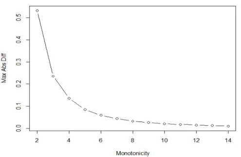
3.6 Determination of Monotonicity . . . 55
3.7 Simulation Studies . . . 55
3.8 Data Analysis . . . 56
CHAPTER 4: COMPETING RISKS · · · 66
4.1 Introduction . . . 66
4.2 Density under Recurrence Times . . . 69
4.3 Non-Parametric Estimation . . . 71
4.3.1 Previous Work . . . 71
4.3.2 Methods . . . 72
4.4 Consistency and Convergence Rate . . . 73
4.5 Asymptotic Distribution . . . 75
4.6 Simulations for Parametric Estimation . . . 75
4.7 Data Analysis . . . 77
CHAPTER 5: DISCUSSIONS AND FUTURE PROJECTS · · · 84
5.1 AFT model for Recurrence Time . . . 84
5.2 Censored 2-Monotone Data . . . 86
5.3 Competing Risks . . . 88
APPENDIX A: TECHNICAL DETAILS FOR CHAPTER 2 · · · 90
APPENDIX B: TECHNICAL DETAILS FOR CHAPTER 3 · · · 97
APPENDIX C: TECHNICAL DETAILS FOR CHAPTER 4 · · · 99
LIST OF TABLES
LIST OF FIGURES
1.1 Pictorial Representation of FRT and BRT · · · 2
3.1 Example of a 2-Monotone Density Estimate · · · 46
3.2 Invelope Function · · · 59
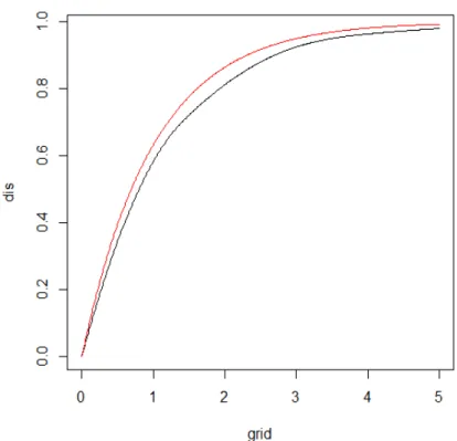
3.3 k-monotone Density Estimates for the Exponential Distribution. · · · 60
3.4 Obtaining k-monotone Density Estimates for a 5-Monotone Density. · · · 60
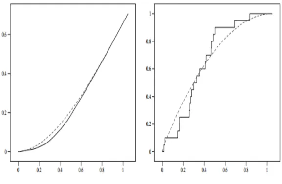
3.5 Density Estimation, p= 0.3 · · · 61
3.6 Distribution Estimation, p= 0.3 · · · 62
3.7 Distribution of Age in the Two Groups. · · · 63
3.8 Density Estimates for the ARIC data in the Presence of Censoring. · · · · 64
3.9 Historam of the uncensored observations in the ARIC data. · · · 65
4.1 Example of Subdistributions · · · 68
4.2 Estimates of the Subdistribution of Stroke for the ARIC Data. · · · 80
4.3 Estimates of the Subdistribution of Heart Failure for the ARIC Data. · · · 81
CHAPTER 1: INTRODUCTION
A prevalent cohort consists of subjects who have experienced an initiating event, like disease onset, prior to their entry to the study and who are followed forward in time until another (terminating) event, like death or symptom development. Sampling may be achieved in a small cross-section. In some prevalent cohort study the onset time may be unobservable as in HIV sero-prevalence studies (Brookmeyer and Gail 1987) where the time of infection to HIV is unknown and interest lies in the follow-up time from enrollment to AIDS. Such prevalent cohorts do not provide information on the time between the initiating event and the terminating eventT, but only provide partial information in terms of the forward recurrence time Tf, the time from sampling to the
terminating event time.
In other scenarios, the time of the initiating event may be known but there may not be any subsequent follow-up after cross-sectional sampling. This is known as the current duration study design, which is encountered, for example, in time to pregnancy surveys. In Keiding et al. (2002), the authors show that the distribution of the times from initiating attempt to cross-sectional sampling for couples that are currently at-tempting to get pregnant, identifies the distribution of the realized time to pregnancy or unsuccessful end of attempt. Another similar study based on current durations is Yamaguchi’s mover-stayer study (Yamaguchi 2003). Such studies provide information on the backward recurrence time Tb.
Figure 1.1: Pictorial Representation of FRT and BRT
originating event and the terminating event) was shorter than the cross-section time, then that data point would never be included in the study. Thus, longer times are favored in the sample. Hence, it is length biased.
1.1 Estimation of the Regression Parameter in the AFT model
In both prevalent cohort and current duration study designs, only subjects who have experienced the initiating event prior to sampling, but have not yet experienced the terminating event can be sampled. Thus both the forward and the backward recurrence times are length biased i.e. the sample is biased towards larger values of T. One way to model this bias (Cox (1969), Vardi (1982)) is to sample proportionally to length, i.e., ifFT is the distribution ofT then the length-biased version TLB has a distribution
given by
FLB(t) = ´t
0 udFT(u)
µT
whereµT = ´∞
0 udFT(u).
Further, if it can be assumed that the incidence of the disease follows a stationary Poisson process then the cross-sectional sampling time is distributed uniformly between the onset time and the terminating time (Cox (1969), Van Es et al. (2000), Keiding et al. (2002)). ThusTf =TLBV, whereV is uniform(0,1). It follows that ifST = 1−FT
is the survival function of T then for both Tf and Tb (commonly denoted as ˜T here),
the density gT˜ is given by
gT˜(t) = ST
µT
. (1.1)
Another interesting way to look at it is the sum of the forward and backward recurrence time data. This sum yields the total length-biased time(TLB) which is known
as Stirling’s interval. Given the total length-biased data, the backward recurrence time follows a Uniform(0, TLB) distribution. So, one can start with the length-biased data
and work backwards to estimate the recurrence time data. If both Tf and Tb are
(Asgharian et al. 2002), (Asgharian and Wolfson 2005) derived the NPMLE for the unbiased incident-case survival function obtained from length-biased prevalent cohort data. The conditional perspective has been investigated by Wang et. al. (Wang et al. (1986), Wang (1991), Wang et al. (1993)). Wang et al. (1986) showed that when the truncating distribution is left completely unspecified, then there is little loss of information when the likelihood is conditioned on the truncation times.
In the presence of covariates, a popular semiparametric model is the proportional hazards (PH) model (Cox 1972) given by
λT|Z(t) =eθ
0Z λ(t),
where,λT|Z is the hazard function ofT given the covariate vectorZ andλis an
unspec-ified baseline hazard function. Here the density ofT is given byeθ0zλ(t)e−eθ 0z
Λ(t), where, Λ is the cumulative hazard satisfying Λ(0) = 0. For the uncensored case, estimates for (θ, λ) can be derived using the partial likelihood based on risk sets (Cox 1972). For right censored data Tsiatis (1981) derives consistency and asymptotic normality of the maximum partial likelihood estimator for θ. Klaassen (1989) showed that the estima-tor is also semiparametric efficient. Details can also be found in Bickel et al. (1993), Murphy and Van der Vaart (2000) and Van der Vaart (1998).
For length-biased data arising out of left-truncation, Wang (1996) derives a con-sistent and asymptotically normal estimator for θ based on a modification of the risk set in order to adjust for the length-bias. Wang defines indicator variables ∆j(ti) for
ti ≤tj, which equals 1 with probabilityti/tj and 0 with probability 1−ti/tj and defines
the modified risk set as
Ri∗ ={j :ti ≤tj,∆j(ti) = 1}.
i.e., the conditional probability of theith subject to die at time ti given that there is a
death from the risk setR∗i is given by
eθ0zi P
j∈R∗i eθ
0z
j.
Thus estimation of θ can be carried out by maximizing the above (pseudo) partial likelihood.
Under cross-sectional sampling of length-biased forward recurrence times, it is not clear how to modify the risk set in order to adjust for the selection bias. Brookmeyer and Gail (1987) discuss the different directions of the bias that might result from fitting a naive proportional hazards model to this kind of data arising out of prevalent cohort studies, where, the onset time of disease is unobservable.
The major difficulties in carrying out semiparametric inference for θ under the PH model and using forward or backward recurrence time data are:
1. Since the Cox model specifies the covariate effect on the hazard function and not the time variable itself, the effect of length-biased cross-sectional sampling on the covariate distribution is intractable. We shall see below that for the accelerated failure time model, this is not a problem.
2. Even if a naive analysis conditioned on Z is carried out, the derivation of the efficient score and information seems difficult. Consider the simplest case of uncensored backward recurrence times where we observe Y = (Tb, Z). The log-likelihood for the
naive analysis conditional on the covariates is given by
lθ,Λ(t, z) = −eθ 0z
Λ(t)−log
ˆ
e−eθ 0
zΛ(t)
The ordinary score forθ is
˙
lθ,Λ(t, z) = −zeθ 0z
(
Λ(t)−
´
e−eθ 0z
Λ(t)Λ(t)dt
´
e−eθ0zΛ(t)dt )
.
Consider the parametric path η 7→ Λη(t) = ´t
0(1 +ηh)dΛ(s), where h ∈ L2(Λ) and |η| ≈0. Replacing Λ by Λη in the log-likelihood and differentiating at η= 0 we get the
score for the nuisance parameter Λ as:
Aθ,Λh=eθ 0z
(ˆ t
0
h(s)dΛ(s) +
´
e−eθ 0z
Λ(t)´t
0 h(s)dΛ(s)dt
´
e−eθ0zΛ(t)
dt
)
.
Deriving the adjoint operatorA∗θ,Λ(Murphy and Van der Vaart 2000) here is not straight forward as in the usual Cox model. As far as we know, a systematic study of forward and backward recurrence times under the proportional hazards assumption for the core time variable has yet to be undertaken.
A useful alternative to the PH model to model survival time T in the presence of covariates Z is the Accelerated Failure Time (AFT) model. Under the AFT model
T =eθ0ZU. (1.2)
Here T is the failure time measured from the time of some initiating event like birth and disease onset, θ is a p× 1 regression parameter, Z is a p×1 covariate vector with density h and U a non-negative random variable independent of Z with density g, survival function S and hazard λ(u) = g(u)/S(u).
logT −θ0Z is assumed independent ofZ and the censoring variable C. Estimation of θ based on the least squares approach has been studied by Miller (1976), James and Buckley (1979) and Koul et al. (1981). Linear rank test based procedures using the partial likelihood score have been developed by Tsiatis (1990), Ritov (1990), Wei et al. (1990), Ying (1993), Fygenson and Ritov (1994) and Jin et al. (2003). For various submodels, these estimators are efficient. For example, the Buckley-James estimator is efficient when the true error density is standard normal while Tsiatis’ linear rank test based estimator with unit weights is efficient for a class of extreme value error distributions. The latter is fully efficient if the weight function adaptively estimates λ0/λ, where λ is the hazard function corresponding to the error distribution.
Another important recent development in estimatingθin a tobit model and the one that we will build upon in section 3 for the random right censored case is Cosslett’s (Cosslett (2004)) asymptotically efficient estimator via a smoothed self-consistency equation. Without covariates and right censoring, nonparametric estimation of the monotone baseline densityg can be achieved using the Grenander (1956) estimator for a monotone density. For the right censoring case this is generalized by the Denby-Vardi (Denbi and Vardi (1986)) NPMLE. In the uncensored case, Woodroofe and Sun (1993) pointed out a technical difficulty in using the actual likelihood. They show that the Denby-Vardi NPMLE is inconsistent near the origin in the sense that ˆg(0+) does con-verge in probability but the limit is strictly greater than g(0+) almost surely. They propose using a penalized likelihood
Lα(g) = n
X
i=1
logg(ui)−nαg(0+),
for some small t0 >0 and then estimate S(t)/S(t0) by ˆg(t)/ˆg(t0).
1.2 2-monotone Density Estimation Under Censoring
The main motivation for this problem arises from the connection between recur-rence times and k-monotone densities. A density is said to be k-monotone if (−1)jg(j) is non-negative, non-increasing and convex for j = 1(1)k−2. Estimation of functions restricted by monotonicity or other inequality constraints has received much atten-tion. Estimation of monotone regression and density functions goes has been done by Grenander (1956). Asymptotic distribution theory for monotone regression estimators was established by Brunk (1970), and for monotone density estimators by Prakasa Rao (1969). The asymptotic theory for monotone regression function estimators was reex-amined by Wright (1981), and the asymptotic theory for monotone density estimators was reexamined by Groeneboom (1985). The “universal component” of the limit distri-bution in these problems is the distridistri-bution of the location of the maximum of two-sided Brownian motion minus a parabola. Groeneboom (1988) examined this distribution and other aspects of the limiting Gaussian problem with canonical monotone function f0(t) = 2t in great detail. Groeneboom (1985) provided an algorithm for computing this distribution, and this algorithm has recently been implemented by Groeneboom et al. (2001).
the consistency near 0.
The least squares (LS) estimator ˜fn of a convex decreasing density function f0 is defined as a minimizer of the criterion function
Qn(f) =
1 2
ˆ
f(x)2dx−
ˆ
f(x)dFn(x),
overK, the class of convex and decreasing nonnegative functions on [0, ∞).
Our aim for this section is to adapt the existing methods for censored observa-tions by utilizing the fact that the decreasing density assumption leads to well-behaved properties of the estimator.
1.3 Recurrence Time Density Estimation for Competing Risks
In this section, our main goal is to study nonparametric estimation for forward and backward recurrence time data with competing risks in the absence of covariates and censoring. The set-up is as follows. We analyze a system that can fail from K competing risks, where K ∈ N is fixed. The random variables of interest are (X, Y), whereX ∈Ris the failure time of the system, andY ∈ {1, . . . , K}is the corresponding failure cause. We cannot observe (X, Y) directly. Rather, we observe the corresponding recurrence time failure T ∈R. This means that at time T, we observe that the failure occurred and we also observe the failure cause Y . Such data can arise naturally in cross-sectional studies with several failure causes.
The Kaplan-Meier estimator can easily be generalized to include competing risks. Lettj1 < tj2 <· · · < tjkj denote the kj distinct failure times for failures of type j. Let
nji denote the number of subjects at risk just before tji and let dji denote the number
K-M estimator lead to
ˆ Sj(t) =
Y
i:tji<t
(1− dji nji
).
It is interesting to note that ˆSj(t) is exactly the same as the standard K-M estimator
that one would obtain if all failures of type other than j were treated as censored cases. If there are no ties between different types of failure, then
ˆ S(t) = K Y j=1 ˆ Sj(t),
so the K-M estimator of the overall survival is the product of the K-M estimators of the cause-specific survivor-like functions.
The Nelson-Aalen estimator of the cause-specific cumulative hazard is
ˆ Λj(t) =
X
i:tji<t
dji
nji
,
and corresponds to an estimate of the cause-specific hazard λj(t) that takes the value
dji/nji at tji and 0 elsewhere. One can also exponentiate the negative of the
Nelson-Aalen integrated hazard to obtain an alternative estimator of the cause-specific survivor-like function Sj(t).
A non-parametric maximum likelihood estimator of Fj(t) was proposed by Aalen
(1976) and can be thought of as a special case of the Aalen-Johansen theory of es-timation for time-inhomogenous Markov processes (Aalen and Johansen 1978). The estimator, known as the Aalen-Johansen estimator is given by
Fj(t) =
X
i:tji≤t
ˆ S(tj−1)
dji
nji
.
added restriction that fj(t) is decreasing. For this, we also look at estimation under
shape restrictions. Without covariates and right censoring, nonparametric estimation of the monotone baseline densityg can be achieved using the Grenander (1956) estima-tor for a monotone density. The estimate is arrived at by obtaining the least concave majorant of the estimate without any shape restrictions. It can be shown that the con-vergence rate of the Grenander estimator in the general case isn1/3 and its asymptotic distribution is basically a Brownian motion with parabolic drift.
1.4 Overview of the dissertation
In Chapter 2 we look at regression parameter estimation in the AFT model for recurrence time data. The problem however is that these estimators are based on the conditional distribution of the time variable given the covariates. Under length bias sampling, the covariate distribution is functionally dependent on the regression param-eter. Thus a “naive” analysis conditioning on the covariates may result in information loss. We show that if the covariate distribution is left completely unspecified then there is no loss of information under a conditional analysis in section 2.5. We also derive a semiparametric asymptotically efficient estimator for the regression parameter in sec-tion 2.6 and show its efficacy under simulated data settings (Secsec-tion 2.7) as well as actual backward recurrence time data (Section 2.8).
Next, we look at k-monotone density estimation in Chapter 3 and prove the fact that if the original density is k-monotone, the corresponding recurrence time density is (k+1)-monotone. So, we develop an algorithm for the estimation of k-monotone densities in the presence of right censoring (Section 3.3). We show the consistency of the estimator and determine its asymptotic distribution in Sections 3.4 and 3.5 respectively.
CHAPTER 2: REGRESSION PARAMETER ESTIMATION IN THE AFT MODEL
In prevalent cohort survival studies where subjects are recruited at a cross-section and followed prospectively in time, the observed event times are length-biased and further follow a multiplicative censoring scheme. For such studies there is an associated initiation time which may be unknown. In this case we only observe the time from sampling to the event of interest. This is the forward recurrence time. Further, in such cases, standard left-truncation survival analysis methods are not applicable.In other scenarios like current duration studies, the time of the initiating event may be known but there is no subsequent follow-up after sampling. Here we observe the backward recurrence times.
information under a conditional analysis in section 2.5. We also derive a semiparamet-ric asymptotically efficient estimator for the regression parameter in section 2.6 and show its efficacy under simulated data settings (Section 2.7) as well as actual backward recurrence time data (Section 2.8).
Next, we look at k-monotone density estimation and prove the fact that if the original density is k-monotone, the corresponding recurrence time density is (k+1)-monotone. So, we develop an algorithm for the estimation of k-monotone densities in the presence of right censoring (Section 3.3). We show the consistency of the estimator and determine its asymptotic distribution in Sections 3.4 and 3.5 respectively.
2.1 FRT and BRT
A prevalent cohort consists of subjects who have experienced an initiating event, like disease onset, prior to their entry to the study and who are followed forward in time until another (terminating) event, like death or symptom development. Sampling may be achieved in a small cross-section. In some prevalent cohort study the onset time may be unobservable as in HIV sero-prevalence studies (Brookmeyer and Gail 1987) where the time of infection to HIV is unknown and interest lies in the follow-up time from enrollment to AIDS. Such prevalent cohorts do not provide information on the time between the initiating event and the terminating eventT, but only provide partial information in terms of the forward recurrence time Tf, the time from sampling to the
terminating event time.
from initiating attempt to cross-sectional sampling for couples that are currently at-tempting to get pregnant, identifies the distribution of the realized time to pregnancy or unsuccessful end of attempt. Another similar study based on current durations is Yamaguchi’s mover-stayer study (Yamaguchi 2003). Such studies provide information on the backward recurrence time Tb.
In both prevalent cohort and current duration study designs, only subjects who have experienced the initiating event prior to sampling, but have not yet experienced the terminating event can be sampled. Thus both the forward and the backward recurrence times are length biased i.e. the sample is biased towards larger values of T. One way to model this bias (Cox (1969), Vardi (1982)) is to sample proportionally to length, i.e., ifFT is the distribution ofT then the length-biased version TLB has a distribution
given by
FLB(t) = ´t
0 udFT(u)
µT
, t ≥0,
whereµT = ´∞
0 udFT(u).
Further, if it can be assumed that the incidence of the disease follows a stationary Poisson process then the cross-sectional sampling time is distributed uniformly between the onset time and the terminating time (Cox (1969), Van Es et al. (2000), Keiding et al. (2002)). ThusTf =TLBV, whereV is uniform(0,1). It follows that ifST = 1−FT
is the survival function of T then for both Tf and Tb (commonly denoted as ˜T here),
the density gT˜ is given by
gT˜(t) = ST
µT
. (2.1)
If both Tf and Tb are observed then standard left-truncated techniques apply. For
has been extensive work towards estimating the length-biased distribution. Two com-mon approaches found in the literature for left-truncated data, are the conditional and the unconditional likelihood approaches, where the conditioning is applied to the on-set times. In the unconditional approach it is assumed that the distribution of the left truncation times are uniformly distributed, which holds under a certain station-arity condition discussed below. In the conditional approach one simply assumes the truncation distribution to be degenerate at the observed truncation times. In the un-conditional approach, Vardi (1982) derived the non parametric maximum likelihood estimator (NPMLE) for the length-biased distribution arising out of prevalent cohorts. Asgharian and Wolfson (Asgharian et al. 2002), (Asgharian and Wolfson 2005) derived the NPMLE for the unbiased incident-case survival function obtained from length-biased prevalent cohort data. The conditional perspective has been investigated by Wang et. al. (Wang et al. 1986), (Wang 1991), (Wang et al. 1993). Wang et al. (1986) showed that when the truncating distribution is left completely unspecified, then there is little loss of information when the likelihood is conditioned on the truncation times.
2.2 Cox Proportional Hazards Model
In the presence of covariates, a popular semiparametric model is the proportional hazards (PH) model (Cox 1972) given by
λT|Z(t) =eθ
0Z λ(t),
where,λT|Z is the hazard function ofT given the covariate vectorZ andλis an
unspec-ified baseline hazard function. Here the density ofT is given byeθ0zλ(t)e−eθ0zΛ(t)
right censored data Tsiatis (1981) derives consistency and asymptotic normality of the maximum partial likelihood estimator for θ. Klaassen (1989) showed that the estima-tor is also semiparametric efficient. Details can also be found in Bickel et al. (1993), Murphy and Van der Vaart (2000) and Van der Vaart (1998).
If we assume a PH model for the coreT, then by (2.1), under length-biased and cross-sectional sampling, the conditional density of the forward or the backward recurrence time ˜T, given Z, is given by
gT˜|Z=z(t) =
e−eθ0zΛ(t)
´
e−eθ0zΛ(t)
and the conditional hazard is given by
λT˜|Z=z(t) =
e−eθ0zΛ(t)
´∞
t e
−eθ0zΛ(u)
du
Thus going from T to ˜T the proportional hazard structure is lost unless, either the baseline hazard is constant or when T given Z follows a Pareto distribution (Van Es et al. 2000). Note that the former case of an exponential distribution can be obtained as a limiting case of the Pareto distribution. Thus usual techniques of estimating θ using the PH model will not apply in general for forward and backward recurrence times. Furthermore, a naive PH model based analysis on ˜T may produce biased estimates.
2.3 Length-Biased Data
For length-biased data arising out of left-truncation, Wang (1996) derives a con-sistent and asymptotically normal estimator for θ based on a modification of the risk set in order to adjust for the length-bias. Wang defines indicator variables ∆j(ti) for
the modified risk set as
Ri∗ ={j :ti ≤tj,∆j(ti) = 1}.
This allows the individuals in the risk setRi∗ to have the population risk set structure, i.e., the conditional probability of theith subject to die at time ti given that there is a
death from the risk setR∗i is given by
eθ0zi P
j∈R∗
i e
θ0z
j.
Thus estimation of θ can be carried out by maximizing the above (pseudo) partial likelihood.
Under cross-sectional sampling of length-biased forward recurrence times, it is not clear how to modify the risk set in order to adjust for the selection bias. Brookmeyer and Gail (1987) discuss the different directions of the bias that might result from fitting a naive proportional hazards model to this kind of data arising out of prevalent cohort studies, where, the onset time of disease is unobservable.
The major difficulties in carrying out a semiparametric inference for θ under the PH model and using forward or backward recurrence time data are:
1. Since the Cox model specifies the covariate effect on the hazard function and not the time variable itself, the effect of length-biased cross-sectional sampling on the covariate distribution is intractable. We shall see below that for the accelerated failure time model, this is not a problem.
naive analysis conditional on the covariates is given by
lθ,Λ(t, z) = −eθ 0z
Λ(t)−log
ˆ
e−eθ 0z
Λ(t)dt.
The ordinary score forθ is
˙
lθ,Λ(t, z) = −zeθ 0z
(
Λ(t)−
´
e−eθ 0z
Λ(t)Λ(t)dt
´
e−eθ0zΛ(t)dt )
.
Consider the parametric path η 7→ Λη(t) = ´t
0(1 +ηh)dΛ(s), where h ∈ L2(Λ) and |η| ≈0. Replacing Λ by Λη in the log-likelihood and differentiating at η= 0 we get the
score for the nuisance parameter Λ as:
Aθ,Λh=eθ 0z (ˆ t 0 h(s)dΛ(s) + ´
e−eθ 0z
Λ(t)´t
0 h(s)dΛ(s)dt
´
e−eθ0zΛ(t)
dt
)
.
Deriving the adjoint operatorA∗θ,Λ(Murphy and Van der Vaart 2000) here is not straight forward as in the usual Cox model. As far as we know, a systematic study of forward and backward recurrence times under the proportional hazards assumption for the core time variable has yet to be undertaken.
2.4 Accelerated Failure Time Model
A useful alternative to the PH model to model survival time T in the presence of covariates Z is the Accelerated Failure Time (AFT) model. Under the AFT model
T =eθ0ZU. (2.2)
with density h and U a non-negative random variable independent of Z with density g, survival function S and hazard λ(u) = g(u)/S(u).
The problem of estimating θ in presence of the nuisance parameters g and h have been taken up by many authors. Two popular approaches are least-squares and rank based procedures. Bickel et al. (1993) derived the semiparametric efficient score and the efficient information for estimating θ when g and h are unspecified and given Z, logT −θ0Z is assumed independent ofZ and the censoring variable C. Estimation of θ based on the least squares approach has been studied by Miller (1976), James and Buckley (1979) and Koul et al. (1981). Linear rank test based procedures using the partial likelihood score have been developed by Tsiatis (1990), Ritov (1990), Wei et al. (1990), Ying (1993), Fygenson and Ritov (1994) and Jin et al. (2003). For various submodels, these estimators are efficient. For example, the Buckley-James estimator is efficient when the true error density is standard normal while Tsiatis’ linear rank test based estimator with unit weights is efficient for a class of extreme value error distributions. The latter is fully efficient if the weight function adaptively estimates λ0/λ, where λ is the hazard function corresponding to the error distribution.
Another important recent development in estimatingθin a tobit model and the one that we will build upon in section 3 for the random right censored case is Cosslett’s (Cosslett (2004)) asymptotically efficient estimator via a smoothed self-consistency equation.
probability but the limit is strictly greater than g(0+) almost surely. They propose using a penalized likelihood
Lα(g) = n
X
i=1
logg(ui)−nαg(0+),
where g varies over a class of decreasing left-continuous densities and α > 0 is a smoothing parameter. Keiding et. al. (2002) discuss that another way to avoid this inconsistency near zero is to estimate the survival function of T conditioned onT > t0 for some small t0 >0 and then estimate S(t)/S(t0) by ˆg(t)/ˆg(t0).
Under the above assumptions and an application of (2.1) we obtain the joint distri-bution of ( ˜T,Z) as˜
fT ,˜Z˜(t, z) =
e−θ0zS(e−θ0zt)
µg
× e
θ0zh(z) ´
eθ0z
h(z)dz. (2.3)
Thus ifT follows the AFT model in (2.2) then, ˜T follows a AFT model given by
˜
T =eθ0Z˜U,˜ (2.4)
where ˜Zhas a density of the formhZ,θ˜ (z) =eθ 0z
h(z)/´ eθ0zh(z)dzand ˜U has a monotone
density given by
gU˜(u) =
S(u)
´∞
0 S(v)dv .
Thus, the resulting AFT model for ˜T has the same covariate effect but a different baseline distribution.
˜
Z) approach, under these restrictive assumptions, result in a gain in semiparametric
information for estimatingθin (2.4). In the next section, we generalize these results to a completely unspecified core covariate distribution and to possibly right censored forward recurrence times. We show that when the core covariate distribution h is completely unspecified, there is no gain in information under an unconditional analysis.
Since the AFT model assumption is preserved under length-biased cross-sectional sampling, a natural question is that whether estimators for θ based on observing (T ∧ C, Z, I{T ≤ C}), where C is a censoring variable independent of T given Z andδ =I{T ≤C}, are also valid when based on observing ( ˜T∧C,˜ Z, δ). In particular,˜ whether an efficient estimator under (2.2) is also efficient under (2.4). Here ˜C is the censoring variable corresponding to ˜T and δ = I{T˜ ≤ C}. We assume that ˜˜ T and ˜C are independent given ˜Z. The issue here is that length-biased cross-sectional sampling results in the density ˜Z to be functionally dependent on θ and thus might contain information about θ unlike the usual set-up where the covariates are ancillary for the regression parameter θ.
In section 2.5 we derive the semiparametric efficient score and information for esti-mating θ based on the data ( ˜Ti∧C˜i,Z˜i,δ˜i), i = 1,· · · , n, while leaving the covariate
distributionh completely unspecified. In section 2.6 we derive an asymptotically semi-parametric efficient estimator for θ. Results from numerical studies are presented in section 2.7 and results from the data analysis are shown in section 2.8.
2.5 Efficient Score and Estimation
We first take up the calculation of the efficient score and information for the forward recurrence time (Tf), subject to right censoring. Let θ ∈Θ, where Θ is a compact set
in<k. Letθ
in terms of the distribution of U(θ) = e−θ0Z˜Tf = e−(θ−θ0)
0Z˜˜
U and the corresponding censored variable Uc(θ) = e−θ0Z˜C. The conditional distribution of˜ U(θ) given ˜Z =z is
gU(θ)(u) =
e(θ−θ0)0zS(e(θ−θ0)0zu)
´
S(v)dv ,
while the conditional hazard is given by
λU(θ)(u) =
S(e(θ−θ0)0zu)
´∞
u S(e(θ
−θ0)0zw)dw.
Note that given ˜Z the distribution of U(θ) is monotonic. We now make the following assumptions:
A1: Tf and ˜C are independent given ˜Z.
A2: µg = ´
S(v)dv <∞.
A3: EgU2λ(U) = ´
u2g2S−1(u)du <∞.
Remark 1. The independent censoring assumption is valid here asC˜ is also measured from the time of sampling. Assumption (A3) is needed to ensure that the density of
U(θ) has finite Fisher information for location.
Let G be the class of density functions on <+ and H be a class of density function on<k. The semiparametric model for the core AFT model in (2.2) is given by
P∗ ={Pθ,g,h : θ∈Θ, g ∈ G, h∈ H},
where, the distribution Pθ,g,h has a density with respect to an absolutely continuous
measureµ given by
dPθ,g,h
dµ (t) =e
For the AFT model for forward recurrence times the semiparametric model is
P =Pθ,Sg,h: θ ∈Θ, g ∈ G, h∈ H
0
, (2.5)
whereSg(u) = ´∞
u g(v)dv for g ∈ G, and
H0 =
h:h∈ H,
ˆ
eθ0zh(z)d(z)<∞,
ˆ
z2eθ0zh(z)dz <∞, θ∈Θ
.
We assume that Θ is a compact subset of Rk. Further, P
θ,Sg,h is dominated by an
absolutely continuous measure µwith density
d
dµPθ,Sg,h =
e(θ−θ0)0zS
g(e(θ−θ0)
0z u)
´
Sg(v)dv
× e
θ0zh(z) ´
eθ0z
h(z)dz.
Define S = {Sg :g ∈ G}. Let the true distribution be P0 = Pθ0,S0,h0 with S0 = Sg0. Define the submodels
Pθ = {Pθ,S0,h0 :θ ∈Θ}, PS = {Pθ0,S,h0 :S ∈ S}and Ph = {Pθ0,S0,h :h∈ H
0}.
Let ˙Pθ, ˙PS and ˙Ph be the respective tangent spaces for Pθ,PS and Ph at P0 = Pθ0,S0,h0. Let ˙lθ be the ordinary score for θ when S and h are fixed. Then the efficient score function ˜lθ ∈(L02(P0))k for θ in the full modelP atP0 is ˜lθ = ˙lθ−Π0( ˙lθ|P˙S+ ˙Ph),
where Π0(l|Q) denotes the orthogonal projection of l onto the linear span ofQ(Bickel et al. (1993)).
The next lemma helps identify ˙PS, i.e., the tangent space for the nuisance parameter
dense set in the maximal tangent spaceL02(S).
Lemma 2. Consider the semiparamatric model P ={Pg :g ∈ G}, where the
distribu-tion Pg has density pg(u) =Sg/ ´
Sg and G is a collection of densities on R+. Let G˙g
and P˙g be the tangent sets for the models G and P respectively at g. If Ag is the score
operator mapping tangents inG˙g to P˙g then, AgG˙g is dense in the maximal tangent set
L02(S) for P.
The proof of this lemma is given in Appendix A.
Theorem 3. Suppose that the covariate vectorZ˜is almost surely bounded. Then under (A1)–(A3) and with φ(u) = 1−ug(u)/S(u) and
M(t) = I{U(θ)≤t} −
ˆ t
0
I{U(θ)> s}λU(θ)(s)ds, (2.6)
the ordinary score for θ at θ =θ0 is
˙ lθ0 =z
ˆ Uc(θ
0) 0
Rφ(s)dM(s)−(z−EZ˜), (2.7)
the tangent space P˙S for S is {l˙Sb : b ∈ L02(S)} where the score operator l˙S for S is
given by
˙ lSb=
ˆ Uc(θ
0) 0
Rb(s)dM(s), (2.8)
the tangent space for h is {b :b ∈L2(h),
´
b(z)eθ00zh(z)dz = 0}, and the efficient score for θ at θ=θ0 is
˜ lθ,S =
ˆ Uc(θ
0) 0
(z−E{Z|U˜ c(θ
0)≥s})Rφ(s)dM(s), (2.9)
where for a ∈L02(S),
Ra(t) = a(t)−
´∞
t´a(u)S(u)du
∞
t S(u)du
The proof of this theorem is attached in Appendix A.
Remark 4. The efficient score is free of h. Thus for estimating θ efficiently we do not
need to estimate the covariate distribution. Thus we do not need a separate
identifiabil-ity condition for h like the mean-zero condition assumed in Klaasen et al. (2004) and
can be left completely unspecified.
Remark 5. The efficient information is given by
˜ Iθ0 =E
ˆ Uc(θ
0)
0
D( ˜Z, C, θ0, s)D( ˜Z, C, θ0, s)0(Rφ)2(s)dFU(θ0)(s), (2.10)
where D( ˜Z, C, θ0, s) = ( ˜Z −E{Z|˜ Uc(θ0) ≥ s}) and a0 denotes the transpose of the vector a.
The efficient score and the information here are similar to the ones in Bickel et al. (1993) for the censored regression problem based on (T, C, Z) except that in the latter caseφ(u) = 1 +ug0(u)/g(u) while in our caseφ = 1−ug(u)/S(u). The main similarity is that in both situations, the efficient scores do not use information in the marginal distribution of the covariates. The reason behind this is the fact that ˙PS ⊥P˙h. Thus
we construct an asymptotically efficient estimator forθ which could be applied to both these problems.
Remark 6. In terms of the residuals (θ0) = logU(θ0) = logTf −θ00Z with density f, distribution F and hazard function λf =f /(1−F), the efficient score at θ =θ0 is
˜ lθ0,f =
ˆ c(θ
0) −∞
(Z −E{Z|c(θ0)≥s})Rφ(s)dM(s), (2.11)
where φ = f0/f, M(t) = I{(θ0) ≤ t} −
´t
−∞I{(θ0) > s}λf(s)ds and Rφ(t) = φ(t) − E{φ((θ0))|(θ0) > t}. Note that f() = eg(e) when observing T, while f() = eS(e)/´ S
g(v)dv when observing Tf.
We obtain the efficient score for the backward recurrence time case as a cor:
Corollary 7. Let U(θ) = e−θ0zTb and suppose that the covariate vector Z˜ is almost
surely bounded and fU(θ) has finite Fisher information for location. Then with λ(u) =
g(u)/S(u), the efficient score for estimating θ at θ =θ0 is
˜
lθ0,λ= ( ˜Z−EZ)[1˜ −U(θ0)λ(U(θ0))] (2.12)
and the efficient information is given by
E[˜lθ0˜l 0
θ0] =E( ˜Z−E ˜
Z)( ˜Z−EZ˜)0E[1−U(θ0)λ(U(θ0))]2. (2.13)
Proof. The backward recurrence times are uncensored. Thus we take Uc(θ) = ∞, M(t) =I{U(θ)≤t} and Rφ=φ in (10) and (12) to get the desired results.
Remark 8. For the case when h is assumed known, Klaassen et. al. (Klaasen et al.
is given by −(z − EZ˜)uλ(u), while the efficient information is V ar( ˜Z)E[U λ(U)]2. Klaassen et. al. also derive the efficient information under the assumption that the
core covariate distribution has mean zero. In these cases there is a gain in
informa-tion. Such gains are possible by projecting the ordinary score to restricted nuisance
tangent spaces.
2.6 Asymptotically Efficient Estimator
In this section we derive a semiparametric asymptotically efficient estimator of the regression parameter θ in the AFT model based on Severini and Wong’s (Severini and Wong (1992)) profile likelihood approach used to estimate the euclidean parameter in presence of a nuisance parameter. Here one identifies a parametric submodel belonging to the nuisance space that passes through the true parameter point and is least-favorable in the sense of having the least Fisher’s information among all parametric submodels (Severini and Wong (1992), Stein (1956)). The idea of estimating the euclidean param-eter is based on estimating a least-favorable curve and then maximizing the correspond-ing likelihood to obtain M-estimators. For the tobit model, Cosslett(Cosslett (2004)) derives an estimator for the regression parameter based on a smoothed self consistent estimate for the distribution of the errors. We adapt this estimator for the randomly right censored linear regression model. The smoothed self-consistent equation for the NPMLE of the survival function of the errors leads to a least favorable submodel for the hazard function. The corresponding estimated log-likelihood is maximized to get a semiparametric efficient estimator.
For arbitrarily fixed θ define the uncensored residuals by θ = logT −θ0Z and the
censored residuals by c
θ = logC −θ
0Z. Also define e ≡ e
θ = θ ∧cθ, where x∧y
Y = (e, δ, Z). The model is
P ={Pθ,λ :θ∈Θ, λ∈Λ}, (2.14)
where Θ⊂ <andΛ={λ :X 7→ <}with further specification made below. UnderPθ,λ,
θ given Z =z has hazard function λ. Let (θ0, λ0) be the true value of the parameter (θ, λ). Let f0 and S0 be the density and the survival functions corresponding to λ0. UnderPθ,λ0,θhas densityf0(·+(θ−θ0)
0z) and survival functionS
0(·+(θ−θ0)0z). The efficient score and information for estimatingθ is given by Proposition 4.6.1 in BKRW (Bickel et al. (1993)). For the forward and the backward recurrence time considered in section 2, the efficient score and information is given in (2.11). Letζθ,z be the survival
function of cθ given Z =z. We make the following additional assumptions:
(C1) The covariate vector Z is bounded almost surely with density h.
(C2) θ0 belongs to the interior of an open and bounded set Θ⊂ <k. Along with (C1) this gives α≡ess. supθ∈Θ|(θ−θ0)0Z|<∞.
(C3) τ = supt{t : P r[C > exp{t +α} | Z] > 0} exists and is finite and further S0(τ +α)>0.
Remark 9. While conditions (C1) and (C2) are standard, condition (C3) is related to
the standard end of study assumption made on the distribution of T and C in
right-censored data settings. The analysis is thus restricted to an interval e∈(−∞, τ].
Let γθ,z(t) ≡ exp{− ´t
−∞λ0(s+ (θ−θ0)
0z)ds}ζ
θ,z(t) denote the at-risk probability
A standard approach for constructing asymptotically efficient estimators for eu-clidean parameters in presence of a nuisance parameters is the profile likelihood ap-proach of Severini and Wong (Severini and Wong (1992)) where the nuisance param-eter is replaced by a suitable consistent estimate (like the NPMLE) in the efficient estimating equation for the euclidean parameter.
The likelihood p(y;θ, λ) underPθ,λ is given by
p(y;θ, λ) ={λ(eθ)}δexp{− ˆ eθ
−∞
λ(u)du}.
Define the Kulback-Lieber distance as,
κ(θ, λ) =−
ˆ
logp(y;θ, λ)p(y;θ0, λ0)dy.
After an application of Fubini’s theorem and integration by parts on the integral term inp(y;θ, λ) we get
κ(θ, λ) =−
ˆ ˆ
n
λ0
t+ (θ−θ00z)
logλ(t)−λ(t)
o
γθ0,z(t)h(z)dzdt.
For Severini and Wong’s profile likelihood approach to work one needs to identify a least-favorable parametric submodel which is essentially a smooth curve θ 7→ λθ
through (θ0, λ0), with λθ0 = λ0 such that for any other submodel λ1θ also satisfying λ1θ0 =λ0, we have,
−E0 d2
dθ2 logp(Y1;θ, λθ)
θ=θ0
≤ −E0 d2
dθ2 logp(Y1;θ, λ1θ)
θ=θ0 ,
where E0 is the expectation under Pθ0,λ0. Under model identifiability, it is sufficient to show that for arbitrarily fixed θ, κ(θ, λθ) < κ(θ, λ1θ) for any λ1θ 6= λθ satisfying
Let Ln(θ, λθ) ≡
P
logp(yi;θ, λθ) be the log-likelihood obtained by replacing the
nuisance parameter λ by the least-favorable submodel λθ. Let ˆλθ be an estimator of
λθ which converges toλθ at a rate faster thann−1/4. Then under regularity conditions
the maximizer ˆθn ofLn(θ,λˆθ) is consistent and asymptotic normal with the asymptotic
variance equal to the efficient information (Severini and Wong (1992)).
Cosslett (Cosslett (2004)) derives an efficient estimator for θ in the tobit model by solving the score equation based on the smoothed self-consistent estimator for the error density. Below we derive the smoothed self-consistent estimator ˆλθ for the
right-censored regression problem and show that it converges to a least-favorable submodel denoted byλθ at a raten−ν1, whereν1 >1/4. For consistency and asymptotic normality we also need that ˆλ0θ goes to λ0θ at a rate n−ν2, where ν
1+ν2 ≥1/2. Here λ0θ ≡dλθ/dθ
and ˆλ0θ =dλˆθ/dθ are the total derivatives taken with respect to θ.
Let Gn,θ(t) ≡ n−1
P
I{ej(θ) ≤ t} and Fn,θ(t) ≡ n−1
P
δjI{ej(θ) ≤ t} denote the
empirical distribution functions of the observed residuals and the observed uncensored residuals respectively. Efron’s (Efron (1967)) self consistent equation for an estimator
¯
S for the survival function of the uncensored residuals for right censored is given by
¯ S(t) =
ˆ ∞
t
dGn,θ(u) + ¯S(t) ˆ t
−∞ 1 ¯
S(v)d(Gn,θ−Fn,θ)(u).
It is well known that the Kaplan-Meier survival function satisfies the above equation. In general, smoothing of a function f(vi) of an observation vi can be achieved by
replacing it with ˜f(vi) = h−n1 ´
f(u)K(h−1
n (u−vi))du, with a suitable kernel K and
bandwidth hn. Thus the self consistency equation after smoothing becomes
˜ S(t) = ˆ ¯ K
t−v hn
dGn,θ(v) +
˜ S(t)
ˆ t
−∞
´ 1 hnK
u−v hn
d(Gn,θ −Fn,θ)(v)
˜
where ¯K(u) = ´u∞K(v)dv and ˜S is the smoothed version of ¯S. The above integral equation is linear in 1/S˜ with an explicit solution
ˆ
S ≡Sˆθ(e) = exp
(
−
ˆ e
−∞ ˆ gn,θ(v)
ˆ Gn,θ(v)
dv
)
, (2.15)
where
ˆ
gn,θ(t) =h−n1 ˆ
K h−n1(t−v)dFn,θ(v)
and
ˆ
Gn,θ(t) = ˆ
¯
K h−n1(t−v)dGn,θ(v).
The integral in (2.15) always exists since by construction the right-hand tail of ˆS decreases at the same rate as the tail of the kernel function. The density estimator corresponding to ˆS in (2.15) is
ˆ fθ(t) =
ˆ gn,θ(t)
ˆ Gn,θ(t)
exp ( − ˆ t −∞ ˆ gn,θ(v)
ˆ Gn,θ(v)
dv
)
. (2.16)
The next set of lemmas establish the convergence of ˆgn and ˆGn. Define,
gθ(t) = ˆ
f0(t+ (θ−θ0)0z)ζθ,z(t)h(z)dz, (2.17)
Gθ(t) = ˆ
S0(t+ (θ−θ0)0z)ζθ,z(t)h(z)dz (2.18)
and
λθ(t) =
gθ(t)
Gθ(t)
=
´
λ0(t+ (θ´ −θ0)0z)γθ,z(t)h(z)dz
γθ,z(t)h(z)dz
. (2.19)
While gθ(·) is the conditional density of the observed residuals eθ given δ = 1, times
P{δ = 1}, Gθ(·) is the unconditional survival function of eθ. Similar “estimable”
and James estimator in Ritov (1990).
Consider the submodel θ 7→ λθ given by (2.19). Note that λθ0 = λ0. Consider the parametric submodelλν =λ(1 +νa), where a∈L2(f0). Then,
dκ(θ, λν)
dν
ν=0 =−
ˆ ˆ
a(t){λ0(t+ (θ−θ0)0z)−λ(t)}γθ0,z(t)h(z)dzdt.
Thus, for arbitrarily fixed θ ∈ Θ, κ(θ, λ) is minimized at λ = λθ. Thus λθ is
least-favorable. Also note that
κ(θ, λθ)−κ(θ0, λ0) =−
ˆ ˆ
log λ0(t+ (θ−θ0) 0z)
λ0(t)
+ 1−λ0(t+ (θ−θ0) 0z)
λ0(t)
×λ0(t)γθ0,z(t)h(z)dzdt ≥0,
where the equality holds if and only ifθ=θ0. Thus if we definem(θ)≡Eθ0,λ0log(pθ,λθ/pθ0,λ0) thenm(θ) is maximized atθ =θ0. Let ˆλθ ≡ˆgn,θ/Gˆn,θ. For each n, the log-likelihood is
given by
Ln(θ, λθ) = n
X
i=1
δilogλθ(ei)− ˆ ei
−∞
λθ(u)du
.
Define ˆθ ≡θˆn to be an element of Θ satisfying
Ln(ˆθ,λˆθˆ) = sup
θ∈Θ
Ln(θ,λˆθ). (2.20)
In order to prove consistency, asymptotic normality and efficiency of ˆθ we need uniform convergence of ˆλθ to λθ and ˆλ0θ toλ
0
θ at appropriate rates (Severini and Wong
kernel are needed to establish the asymptotics: (R1) f0, f00 and f
00
0 are bounded. (R2) The functions gθ, gθ0, g
00
θ, Gθ, G0θ, G
00
θ are continuous and uniformly bounded in
θ∈Θ. Here, gθ0 ≡dgθ/dθ and the other derivatives are defined similarly.
(R3) Eθ0,λ0|θ|
p <∞, for some p >4.
(R4) λθ and logλθ have two continuous derivatives. Further, these functions and their
derivatives are bounded by integrable functions for all θ∈Θ.
(K1) K is a bounded, differentiable and symmetric function satisfying ´ K = 1,
´
u2K(u)du <∞, ´[K0(u)]2du <∞and ´[K00(u)]2du <∞.
(K2) The bandwidth hn satisfies hn=n−β, where 1/8≤β <1/5.
Remark 10. While conditions (R1)–(R3) are standard, condition (R4) cannot be
ex-pressed in a more straightforward way in terms of the underlying true error hazard.
It is worthwhile to note that (R4) holds in case the error density is normal and with
bounded covariates.
Lemma 11. Under assumptions (C1) and (C2), the classes F = {δI[eθ ≤ t] : θ ∈
Θ, t ∈R}, G ={ZI[eθ ≤t] :θ ∈Θ, t∈R} and H ={δZI[eθ ≤t] :θ ∈Θ, t ∈R} are
P-Donsker.
Proof. {I[eθ ≤ t] : θ ∈Θ, t ∈R} is P-Donsker since a finite-dimensional vector space
of measurable functions isP-Donsker. LetG(y) be a uniformly bounded function then by the preservation thm {G(y)I[eθ ≤t]}is P-Donsker.
Lemma 12. Under (C1), (C2), (R1)–(R4) and (K1) we have,
(b) |Gˆn,θ(t)−Gθ(t)|=Op(h2n),
(c) |ˆgn,θ0 (t)−g0θ(t)|=Op(n−1/2)Op(h−n2) and
(d) |Gˆ0n,θ(t)−G0θ(t)|=Op(h2n)
uniformly in t and θ ∈Θ,
The proof of this lemma is given in Appendix A.
Lemma 13. Under (C3) and conditions (R1)–(R4) and (K1),
(a) supt|λˆn,θ(t)−λθ(t)|=Op(n−1/2)Op(h−n1) +Op(h2n)
(b) supt|λˆ0n,θ(t)−λ0θ(t)|=Op(n−1/2)Op(h−n2)
uniformly in t ∈I and θ ∈Θ.
Proof. Note that under (C3), (R2) and (K1),
sup
t∈I
|λˆθ(t)−λθ(t)|
≤sup
t∈I
ˆ
gn,θ(t)−gθ(t)
Gθ(t)
+|ˆgn,θ(t)|
ˆ
Gn,θ(t)−Gθ(t)
ˆ
Gn,θ(t)Gθ(t)
!
≤Gθ(τ)−1sup t
|ˆgn,θ(t)−gθ(t)|
+
sup
t
|ˆgn,θ(t)−gθ(t)|+ sup t
|gθ(t)|
G(τ)−1
.
G(τ)−sup
t
|Gˆn,θ(t)−Gθ(t)|
−1
sup
t
|Gˆn,θ(t)−Gθ(t)|.
By lemma 3, the dominating term in the preceding line isOp(|ˆgθ−gθ|). Thus part (a)
follows. A similar inequality for|λˆ0θ−λ0
θ|shows that the dominating term isOp(|ˆgθ0−g
0
θ|)
Remark 14. Note that along with (K2), lem 4 gives the convergence rates of order
n−ν1 with ν
1 ≥ 1/4, for ˆλθ → λθ and of order n−ν2 with ν1+ν2 ≥ 1/2, for λˆ0θ → λ0θ,
uniformly in θ ∈Θ and t < τ.
Define Ln(θ,λˆθ) ≡
P
{δlog ˆλθ(eθ)− ´eθ
−∞λˆθ(u)du} then ˆθn be the maximizer of θ 7→ Ln(θ,λˆθ). In order to show that ˆθn is consistent for θ, we need to show that
n−1L
n(θ,λˆθ)− n−1Ln(θ, λθ) converges to zero uniformly in θ. For isolated terms in
the left tail like an isolated e(1), ˆλθ(e(1)) is of order O(1/nhn), thus we need to use a
trimming factor to avoid any contribution of such terms to Ln(θ,ˆλθ) or to Ln(θ, λθ).
Consider the trimming function τ(·), given by
τ(u) =
1 for u≥1 ψ(u) for 0< u <1 0 for d≤0,
where, in order to makeτ twice differentiable with continuous derivatives we choose a smooth bridge function ψ(·) which is twice differentiable withψ(0) =ψ0(0) = ψ0(1) = ψ00(0) = ψ00(1) = 0 and ψ(1) = 1. Also we let bn ↓ 0 at a suitable rate and define
τ1(λ)≡τ(b−n1(λ−bn)) and
L∗n(θ,λˆθ)≡n−1
X
{δlog ˆλθ(eθ)τ1(ˆλθ(eθ))− ˆ eθ
−∞ ˆ
λθ(u)du}.
Similarly define L∗n(θ, λθ).
Lemma 15. Under assumptions (C1)–(C4) and conditions (R1)–(R4) and (K1) and
(K2), if the trimming rate bn = n−α with 0 < α < 1/4, then,
n
−1L∗
n(θ,ˆλθ) −
n−1Ln(θ, λθ)
P
Proof.
L∗n(θ,λˆθ)−L∗n(θ, λθ)
=n−1Xδ
"
τ1(λθ(eθ)) log
ˆ λθ(eθ)
λθ(eθ)
+ log ˆλθ(eθ){ˆλθ(eθ)−λθ(eθ)}τ10(ˆγ)
#
−n−1X
ˆ eθ
−∞
{ˆλθ(u)−λθ(u)}du.
Now considerτ(λθ) log(ˆλθ/λθ) =τ(λθ) log[1 +λθ−1(ˆλθ−λθ)]. This is zero whenλθ ≤bn.
Thus the worst possible case is when λθ =bn. Now τ(bn) log[1 +bn−1Op(n−1/4)]→0 as
n→ ∞ if bn =n−α with 0< α <1/4.
The second termτ0(γ)(ˆλθ−λθ) log ˆλθ = 0 ifγ < bn orγ >2bn. In the worst possible
case we have γ = ˆλθ+δn = bn where δn =n−β with β ≥ 1/4. Then log ˆλθ = logbn+
log(1−δn/bn). Thusτ0(γ)(ˆλθ−λθ) log ˆλθ =τ0(bn)Op(n−1/4)[logbn+ log(1−δn/bn)]→0
asn → ∞since δn/bn→0.
A similar Taylor’s expansion inside the integral term yields,
ˆ eθ
−∞
τ(λθ)(ˆλθ−λθ)(u)du≤Op(n−1/4)[n−1
X
eθ−mn],
where mn = sup{t :λθ(t)≤ bn}. Note that for exponential and sub-exponential tails,
mn ↓ −∞ at a rate slower than bn. Also, since, E|eθ| < ∞, the integral term goes
to zero. Thus L∗n(θ,λˆθ)−L∗n(θ, λθ) → 0. Also, since |L∗n(θ, λθ)| ≤ |Ln(θ, λθ)|, under
regularity condition (R4), the bounded convergence thm gives
L∗n(θ, λθ)−Ln(θ, λθ)→E[L∗n(θ, λθ)−Ln(θ, λθ)].
Also, L∗n(θ, λθ) converges to Ln(θ, λθ) point-wise as n → ∞. Thus another use of
Theorem 16. If θˆn is the maximizer of the log-likelihood as in (2.20) then under (C1)–
(C4), (R1)–(R4) and (K1) and (K2), θˆn
P
→θ0 as n→ ∞.
Proof. Let m(θ) ≡ E0Ln(θ, λθ). In section 3.3, we saw that m(θ) is maximized at
θ0. Also by condition (R4) and assumption (A3) we have that Ln(θ, λθ) is a sum of
n bounded terms and thus by the weak law of large numbers n−1L
n(θ, λ) → m(θ)
for every θ ∈ Θ. Under condition (R3) and (R4) and the compactness of Θ and an application of the argmax thm (cor 3.2.2 in van der Vaart and Wellner (1996)), we have ˆ
θn
P →θ0.
For asymptotic normality and efficiency, we use the profile likelihood theory in Murphy and Van der Vaart (Murphy and Van der Vaart (2000)). thm 1 in Murphy and Van der Vaart (2000) provide sufficient conditions under which the log profile likelihood logpln(θ) admits the following asymptotic expansion:
logpln(θ0) + (˜θn−θ0)0
n
X
i=1 ˜
l0(Yi)−
1
2n(˜θn−θ0) 0˜
I0(˜θn−θ0)0 + op(
√
n||θ˜n−θ0||+ 1)2,
Theorem 17. √nθˆn−θ0
D
→N(0,I˜0−1), whereI˜0 is the efficient information matrix.
Proof. Here we adapt to the notation in Murphy and Van der Vaart (Murphy and Van der Vaart (2000)) and apply their main thm. Forη in a neighborhood of θ0 define the map η7→λη(θ, λ) by
λη(θ, λ)(t) = ´
λ(t+ (η´ −θ)0z)γη,z(t)h(z)dz
γη,z(t)h(z)dz
,
whereγη,z is defined in section 3.2. Also define the log-likelihood as
η7→l(η, θ, λ) = logp(y;η, λη(θ, λ))
Let ˙l(η, θ, λ) denote the derivative of η 7→ l(η, θ, λ). Note that λθ(θ, λ) = λ for every
θ and λ in the parameter space and that ˙l(θ0, θ0, λ0) = ˜lθ0,λ0, where ˜l is the efficient score given in (2.11). Thus following (Murphy and Van der Vaart (2000)), the above submodel is least favorable at (θ0, λ0). Under the regularity conditions it can be shown that in a neighborhood V around (θ0, θ0, λ0), {l(η, θ, λ) : (η, θ, λ)˙ ∈ V} is P0-Donsker with square integrable envelope and {¨l(η, θ, λ) : (η, θ, λ)∈ V} is P0-Glivenko-Cantelli. In order to apply theorem 1 in Murphy and Van der Vaart (2000), we need to check the “no-bias” condition given by
E0l(θ˙ 0,θˆn,λˆθˆn) =op(|θˆn−θ0|+n−1/2).
Consider writingE0l(θ˙ 0, θ0, λ) as
E0
pθ0,λ0 −pθ0,λ pθ0,λ0
˙
l(θ0, θ0, λ)−l(θ˙ 0, θ0, λ0)
−E0l(θ˙ 0, θ0, λ0)
pθ0,λ−pθ0,λ0 pθ0,λ0
−A0(λ−λ0)
where,A0 is the score operator for λ at (θ0, λ0) and is given by
A0h=
ˆ e(θ0)
−∞
Rh(s)dM(s),
and R and the martingale M are as in rem 5. Note that E0˜l0A0h = 0 for every h∈L2(f0) by the orthogonality property of the efficient score. Sinceλ 7→pθ0,λ is twice differentiable and λ 7→ l(θ˙ 0, θ0, λ) is differentiable at λ0, taking a first order Taylor’s expansion in the first term in (2.21) and a second order Taylor’s expansion in the second term of (2.21) aroundλ0 we see that the expression in (2.21) is of orderOp(||λ−λ0||2). Thus following the discussion in Murphy and Van der Vaart (2000) it is sufficient to have
||λˆθˆn−λ0||=Op(|θˆn−θ0|) +op(n−1/4),
for the “no-bias” condition to hold.
Since ˆθn is consistent for θ0 and θ 7→λˆθ is differentiable, by lemma 4, we have the
desired result.
2.7 Simulation Studies
As our method is unconditional on the covariate distribution, it is a special case of the model used in the paper by Zeng and Lin (2007) (since we assume that the covariates are constant over time). So, we use their profile likelihood approach to estimate θ and compare it with Klassen’s mean zero approach and also the known covariate structure approach. We consider only 1 covariate Z ∼U nif(−1,1). So, ˜Z has density given by
θeθz
eθ−e−θ, where −1 ≤ z ≤ 1. We take different values of θ and assume that the error
1000 replicates and look at the mean bias and variance in estimating θ. We also look at what happens when the covariate distribution is misspecified.For this, we consider Z∼ (x,1) for some choice of x. So, ˜Z has density given by eθθe−eθz−θx where x≤z≤1.
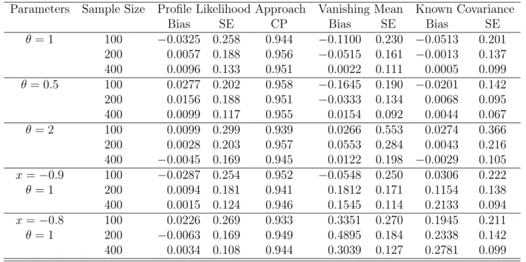
Table 2.1: Estimates for the Backward Recurrence Time Data
Parameters Sample Size Profile Likelihood Approach Vanishing Mean Known Covariance
Bias SE CP Bias SE Bias SE
θ= 1 100 −0.0325 0.258 0.944 −0.1100 0.230 −0.0513 0.201 200 0.0057 0.188 0.956 −0.0515 0.161 −0.0013 0.137
400 0.0096 0.133 0.951 0.0022 0.111 0.0005 0.099
θ = 0.5 100 0.0277 0.202 0.958 −0.1645 0.190 −0.0201 0.142 200 0.0156 0.188 0.951 −0.0333 0.134 0.0068 0.095
400 0.0099 0.117 0.955 0.0154 0.092 0.0044 0.067
θ= 2 100 0.0099 0.299 0.939 0.0266 0.553 0.0274 0.366
200 0.0028 0.203 0.957 0.0553 0.284 0.0043 0.216
400 −0.0045 0.169 0.945 0.0122 0.198 −0.0029 0.105 x=−0.9 100 −0.0287 0.254 0.952 −0.0548 0.250 0.0306 0.222
θ= 1 200 0.0094 0.181 0.941 0.1812 0.171 0.1154 0.138
400 0.0015 0.124 0.946 0.1545 0.114 0.2133 0.094
x=−0.8 100 0.0226 0.269 0.933 0.3351 0.270 0.1945 0.211
θ= 1 200 −0.0063 0.169 0.949 0.4895 0.184 0.2338 0.142
400 0.0034 0.108 0.944 0.3039 0.127 0.2781 0.099
Thus, we find that the estimates obtained using our methods are quite comparable to the special case where the covariance structure is known, though Klassen’ methods have lesser variance. However, their estimates are very sensitive to model specification. On the other hand, our naive analysis yields unbiased estimates in both cases. The variance estimators accurately reflect the actual variance, while the confidence intervals have correct coverage probabilities.
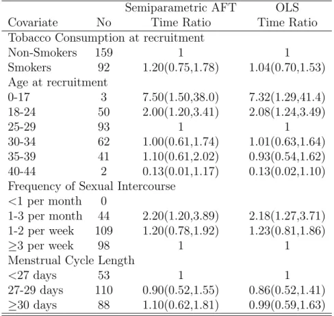
2.8 Data Analysis
For the data analysis, we use a subset of the data used by Keiding et al (2012). It is a backward recurrence time data on the time to pregnancy obtained from a large French telephone survey. Women were eligible if they were between 18-44 years old, were living with a male partner and did not use any method to avoid pregnancy. We consider only nulliparous women who had not initiated any fertility treatment. The response variable was the current duration of unprotected intercourse, which is the time elapsed from the start of unprotected intercourse and the interview.
Table 2.2: Estimates for time ratios and the CI for nulliparous women Semiparametric AFT OLS
Covariate No Time Ratio Time Ratio
Tobacco Consumption at recruitment
Non-Smokers 159 1 1
Smokers 92 1.20(0.75,1.78) 1.04(0.70,1.53) Age at recruitment
0-17 3 7.50(1.50,38.0) 7.32(1.29,41.4)
18-24 50 2.00(1.20,3.41) 2.08(1.24,3.49)
25-29 93 1 1
30-34 62 1.00(0.61,1.74) 1.01(0.63,1.64) 35-39 41 1.10(0.61,2.02) 0.93(0.54,1.62) 40-44 2 0.13(0.01,1.17) 0.13(0.02,1.10) Frequency of Sexual Intercourse
<1 per month 0
1-3 per month 44 2.20(1.20,3.89) 2.18(1.27,3.71) 1-2 per week 109 1.20(0.78,1.92) 1.23(0.81,1.86)
≥3 per week 98 1 1
Menstrual Cycle Length
<27 days 53 1 1
CHAPTER 3: TWO-MONOTONE DENSITY ESTIMATION IN THE PRESENCE OF RIGHT CENSORING
3.1 Introduction
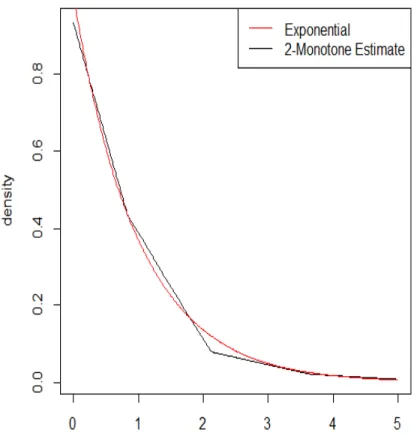
A density function g on R+ is monotone (or 1-monotone) if it is nonincreasing. It is 2-monotone if it is nonincreasing and convex, and k-monotone for k ≥ 3 if and only if (−1)jg(j) is nonnegative, nonincreasing and convex for j=1(1)k-2. Figure 3.3 shows an estimate of a 2-monotone density for the standard exponential distribution for a sample size of 100, under no censoring.
Estimation of functions restricted by monotonicity or other inequality constraints has received much attention. Estimation of monotone regression and density functions goes has been done by Grenander (1956). Asymptotic distribution theory for mono-tone regression estimators was established by Brunk (1970), and for monomono-tone density estimators by Prakasa Rao (1969). The asymptotic theory for monotone regression function estimators was reexamined by Wright (1981), and the asymptotic theory for monotone density estimators was reexamined by Groeneboom (1985). The “universal component” of the limiting distribution in these problems is the distribution of the lo-cation of the maximum of two-sided Brownian motion minus a parabola. Groeneboom (1988) examined this distribution and other aspects of the limit Gaussian problem with canonical monotone function f0(t) = 2t in great detail. Groeneboom (1985) provided an algorithm for computing this distribution, and this algorithm has recently been implemented by Groeneboom et al. (2001).
Figure 3.1: Example of a 2-Monotone Density Estimate
(1994), who was motivated by some problems involving the migration of birds dis-cussed by Hampel (1987). Jongbloed established lower bounds for minimax rates of convergence and established rates of convergence for a“sieved maximum likelihood es-timator”. Finally, a least squares estimator as well as a non-parametric maximum likelihood estimator for 2-monotone densities were established by Groeneboom et al. (2001) which were further modified by Balabdaoui and Wellner (2007) to correct for the consistency near 0.