STATISTICAL METHODS FOR REPEATED MEASURES IN EXPERIMENTAL GINGIVITIS WITH ADJUSTMENT FOR LEFT
TRUNCATION DUE TO LOWER DETECTION LIMITS
Kelley D. Wekheye
A dissertation submitted to the faculty of the University of North Carolina at Chapel Hill in partial fulfillment of the requirements for the degree of Doctor of Public Health
in the Department of Biostatistics, Gillings School of Global Public Health.
Chapel Hill 2014
Approved by:
John S. Preisser
Lloyd J. Edwards
Anastasia Ivanova
Steven Offenbacher
ABSTRACT
KELLEY D. WEKHEYE: Statistical Methods For Repeated Measures In Experimental Gingivitis With Adjustment For Left Truncation Due to
Lower Detection Limits
(Under the direction of John S. Preisser)
In the characterization of biomarkers measured repeatedly over time, there is a need
to summarize the information contained in the multivariate data. In experimental
gin-givitis (EG), for example, biomarker levels change when the benefits of toothbrushing
are withheld during an induction phase, then restored during a resolution phase. The
pattern of change over time of biomarker levels associated with gingivitis could reflect
change in various directions; therefore, the statistical methodology utilized should
con-sider this possibility. As such, area under the curve (AUC) can be implemented as
a summary measure for estimating change in biomarker levels. Parametric statistical
models for repeated measures analysis are useful for characterizing the nature of that
change over time, particularly as they easily accommodate both truncated and missing
data. In EG studies, left truncation results when a biomarker level falls below the
lower limit of detection. We propose two parametric approaches to provide direct
esti-mation of the trends in biomarkers over time while implementing adjustments for left
truncation. The focus is on estimation and hypothesis testing for AUC.
The first paper derives a piecewise linear random-effects regression model fit to 3
biomarkers representing varying degrees of missingness due to lower detection limits
using 2 ad hoc (naive) approaches for handling non-detect values and a likelihood
approach accounting for left censoring (Lyles, Lyles and Taylor, 2000). These naive
limit, which may result in bias, while the maximum likelihood method gives valid results
when dropouts are missing at random.
The second paper outlines AUC methodology for repeated measures biomarker data
by using a nonlinear “Gamma Curve” mixed model with adjustment for left truncation
based on a maximum likelihood approach in comparison to the ad hoc approaches
outlined in the first paper.
The third paper presents a simulation study that includes methods from the first
two papers as well as Wilcoxon Sign Rank test methods from Preisser, Sen, and
Offen-bacher (2011). The simulation design, motivated by EG studies, focuses on properties
of hypothesis tests (size and power) in the presence of left truncation and/or
miss-ing data to evaluate whether the parametric methods are reliable for small sample
sizes or whether larger samples are needed to reliably use the methods. Evidence for
recommending certain sample sizes for EG studies and an evaluation of whether the
nonparametric method is robust to left truncation and crude single imputation methods
are also provided.
The proposed methodology is illustrated using longitudinal data from an EG study
whereby the benefits of toothbrushing are temporarily withheld, then restored
To my dad, Nathaniel Peterson, for his love and dedication shown in raising two little
girls on his own after the passing of his wife. To my mom, Geraldine Peterson, in
loving memory. Her presence made me the woman I am today, motivated me to strive
ACKNOWLEDGMENTS
First, all praise, honor, and glory to my Heavenly Father for making this degree
even possible. Secondly, I am particularly thankful and grateful for my dear husband
Chrisantos for his continuous encouraging words, love, support, and extreme patience
during this process. We have gone through a lot together during this process and have
come out victorious.
I would like to express my sincere gratitude to my academic and dissertation advisor,
Dr. John S. Preisser. Without his guidance, it would have been challenging to complete
the DrPH program and to write my dissertation. His support and feedback have been
invaluable. Dr. Preisser has always been available to help and provided me with
insightful references and ideas critical for this dissertation. He graciously reviewed
several versions of the papers, and his suggestions have substantially contributed to
the quality of my work.
I am very appreciative of the tremendous support of Dr. Lloyd Edwards. His
supe-rior knowledge of substantive issues concerning repeated measures analysis provided a
unique perspective to the research problem and helped immensely in the interpretation
of the results.
I am very grateful to Dr. Anastasia Ivanova for her graciousness and helpful
com-ments during this dissertation process.
My heartfelt gratitude goes also to Dr. Steven Offenbacher. Dr. Offenbacher was
kind enough to meet with me and Dr. Preisser early on in the research process to discuss
the topic. He has provided me with insightful information critical for understanding
dissertation. I would also like to thank Dr. Silvana Barros for providing insightful
comments to my first paper.
I would also like to communicate my sincere thanks to Dr. P.K. Sen whose
sugges-tions have helped strengthen the statistical methodology used in this dissertation. Dr.
Sen was kind enough to recommend revisions that greatly enhance the quality of the
manuscript and maintain scientific rigor.
This dissertation would also not have been possible without the prayers and support
of numerous family members and friends. I would like to thank my sister Courtney
Alexander, brother-in-law Cory Alexander, and my niece and nephews for their support,
laughter, and sending gifts during this process. I would also like to thank my best
friends Kyla Kurian (and family) and Rachael Redmond for their prayers, support,
encouragement, and for helping select my final defense attire. You are truly like sisters
to me. Thanks to my two other girlfriends/sisters Elexica McAlister (and family) and
Julie Omishakin (and family) for their prayers and support. Thanks also go to Leon
and Mashall Bullard (and family) for their endless support and encouragement. Special
thanks to Isaiah Redmond and Christopher Paine for always making it a goal of theirs
to keep me laughing whenever I see them.
Lastly, I would like to thank the countless other people who have supported me
in various aspects during the completion of this dissertation, particularly the Kenyan
TABLE OF CONTENTS
LIST OF TABLES. . . xi
LIST OF FIGURES . . . xiii
LIST OF ABBREVIATIONS . . . xiv
1 CHAPTER 1: INTRODUCTION . . . 1
2 CHAPTER 2: LITERATURE REVIEW . . . 4
2.1 Overview of Gingivitis . . . 4
2.2 Overview of the Experimental Gingivitis Study . . . 5
2.3 Review of Design and Analysis Methods in Experimental Gingivitis Studies . . . 6
2.4 Linear Mixed Models . . . 9
2.5 Methods For Left Truncated Data . . . 10
2.6 Area-Under-the-Curve Principle . . . 13
2.7 Univariate and Multivariate Hypothesis Testing Based on Wilcoxon Signed Rank Statistics . . . 15
2.8 Methods for Multiple Hypothesis Testing . . . 17
2.9 Summary and Proposed Research . . . 19
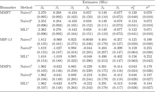
3 CHAPTER 3: PIECEWISE LINEAR MIXED MODEL . . . 22
3.1 Background and Introduction . . . 22
3.4 Example . . . 32
3.5 Results . . . 33
3.5.1 Regression Estimates . . . 33
3.5.2 Estimates, standard errors (SEs), and 95% Confidence Intervals of Area-Under-the-Curve (A, B, C, and D) . . . 37
3.5.3 Estimates and Standard Errors of Summary Indices of Change (X1, X2, X3, and X4) and P-values . . . 40
3.6 Discussion and Conclusion . . . 42
4 CHAPTER 4: NONLINEAR GAMMA-LIKE MIXED MODEL . . 45
4.1 Background and Introduction . . . 45
4.2 Gamma Curve-Like Nonlinear Mixed Model . . . 49
4.3 Maximum Likelihood Estimation in the Presence of Left Truncation . . 53
4.4 Example . . . 54
4.5 Results . . . 56
4.5.1 Regression Estimates . . . 56
4.5.2 Estimates, Standard Errors, and 95% Confidence Intervals of Area-Under-the-Curve (A, B, C, and D) . . . 60
4.5.3 Estimates and Standard Errors of Summary Indices of Change (X1, X2, X3, and X4) and P-values . . . 63
4.6 Discussion and Conclusion . . . 65
5 CHAPTER 5: COMPARISON OF STATISTICAL METHODS . . 66
5.1 Background and Introduction . . . 66
5.2 Statistical Methods . . . 70
5.2.1 Piecewise Linear Mixed Model . . . 70
5.2.2 Gamma Curve-Like Mixed Model . . . 72
5.3 Simulation Studies . . . 77
5.4 Simulation Results . . . 78
5.5 Discussion . . . 83
6 CHAPTER 6: FUTURE RESEARCH . . . 85
6.1 Alternative Models . . . 85
6.2 Multiple Hypothesis Testing . . . 85
APPENDIX A: SAS CODE FOR PIECEWISE MODEL . . . 87
LIST OF TABLES
1 Amount of missingness across biomarkers . . . 33
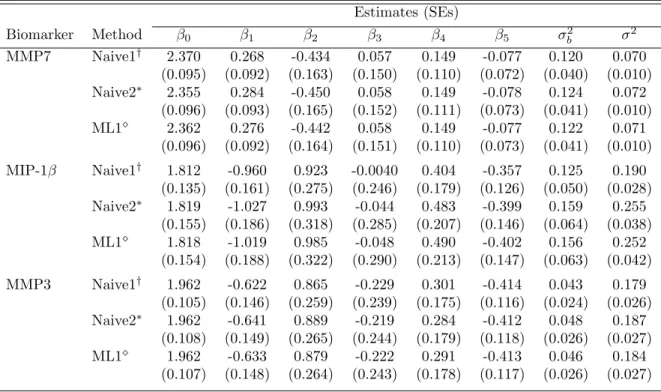
2 Results from experimental gingivitis study using a piecewise linear mixed model: comparing ML estimates from ad hoc approaches with ML esti-mates from an approach accounting for non-detectable values . . . 36
3 Results from experimental gingivitis study using a piecewise linear mixed
model fit in PROC NLMIXED: comparing ML estimates from ad hoc
approaches with ML estimates from an approach accounting for non-detectable values . . . 37
4 Estimates (SEs), and 95% CIs of AUC from experimental gingivitis study using piecewise linear mixed model: comparisons of ad hoc approaches with an approach accounting for non-detectable values . . . 39
5 Estimates (SEs) of summary indices of change and p-values from
ex-perimental gingivitis study using piecewise regression: comparing sig-nificance from ad hoc approaches with significance from ML approach accounting for non-detectable values . . . 42
6 Amount of missingness across biomarkers . . . 55
7 Results from experimental gingivitis study using a nonlinear gamma
curve-like mixed model: comparing ML estimates from ad hoc approaches with ML estimates from an approach accounting for non-detectable values 59
8 Estimates (SEs), and 95% CIs of AUC from experimental gingivitis study using a nonlinear gamma curve-like mixed model: comparisons of ad hoc
approaches with an approach accounting for non-detectable values . . . 62
9 Estimates (SEs) of summary indices of change and p-values from
ex-perimental gingivitis study using a nonlinear gamma curve-like model: comparing significance from ad hoc approaches with significance from ML approach accounting for non-detectable values . . . 64
11 Results from 6 approaches for analyzing experimental gingivitis data based on 1000 datasets simulated from a gamma-curve model with ran-dom intercept and 25% left-truncation . . . 81
LIST OF FIGURES
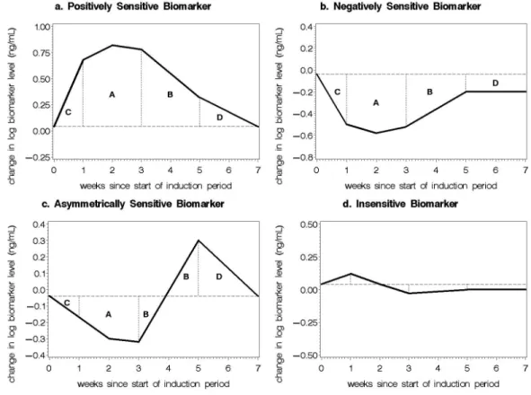
1 Typical biomarker patterns of change over time for experimental
gin-givitis. Letters A, B, C, and D denote a partition of AUC for which summary measures of change can be estimated. . . 26
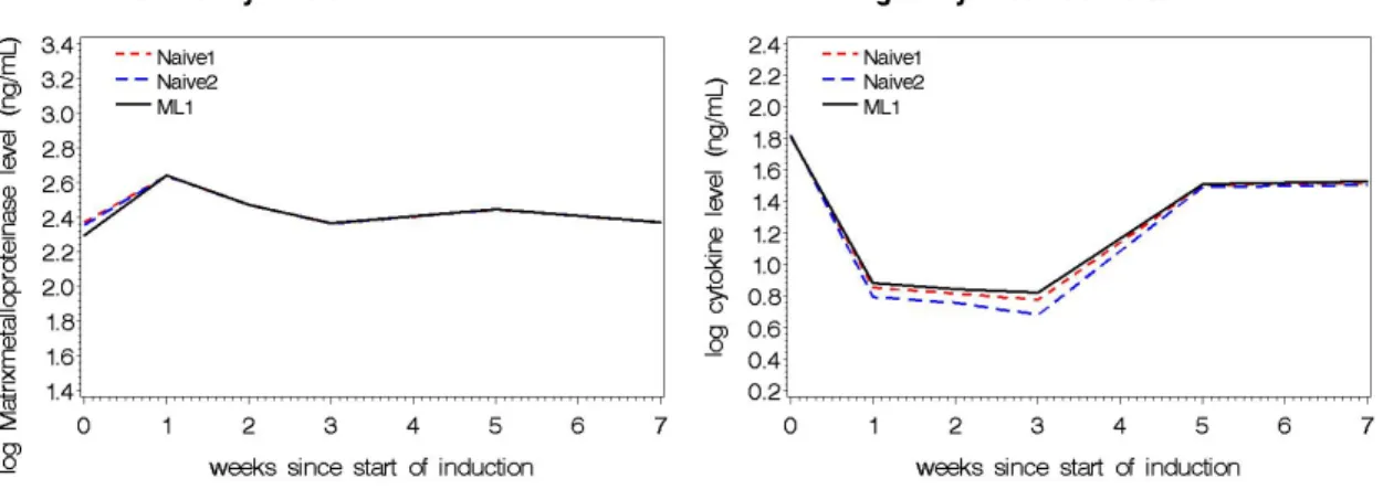
2 Subject-level best linear unbiased predictions and population-averaged biomarker levels over time for MMP7 (upper left), MIP-1β (upper right), and MMP3 (lower center) based on the piecewise linear mixed model. . 34
3 Population-averaged biomarker levels over time for MMP7 (upper left), MIP-1β (upper right), and MMP3 (lower center) for the three ad hoc
methods based on the piecewise linear mixed model. . . 35
4 Typical biomarker patterns of change over time for experimental
gin-givitis. Letters A, B, C, and D denote a partition of AUC for which summary measures of change can be estimated. . . 49
5 Patterns of change over time for positively sensitive biomarker with vari-ation in intercept (β0), shape (β1), scale (β2), and location shift (θ1)
parameters. Panel a: β0=0.04, 0.07, 0.10; β1 = 5.00; β2 = 1.00; θ1 =
2.0. Panel b: β0=0.10; β1 = 5.00; β2 = 1.00; θ1 = 1.0, 2.0, 3.0. Panel c
(solid line): β0=0.10; β1 = 4.00, 4.50, 5.00; β2 = 1.00; θ1 = 2.0. Panel
c (dashed line): β0=0.10; β1 = 5.00; β2 = 1.00, 1.20, 1.40; θ1 = 2.0.
Panel d: β0=0.089, 0.10, 0.116; β1 = 8.19, 5.00, 3.66; β2 = 2.047, 1.00,
0.61; θ1 = 2.0. . . 50
6 Subject-level best linear unbiased predictions and population-averaged biomarker levels over time for MMP7 (upper left), MIP-1β (upper right),
and MMP3 (lower center) based on the gamma curve-like mixed model. 58
7 Population-averaged biomarker levels with 95% pointwise confidence bands
over time for MMP7 (upper left), MIP-1β (upper right), and MMP3
LIST OF ABBREVIATIONS
ANOVA analysis of variance
AS asymmetrically sensitive
AUC area-under-the curve
CI confidence interval
EG experimental gingivitis
EM expectation maximization
FDR false discovery rate
FWER family-wise error rate
GCF gingival crevicular fluid
IS insensitive
LOD limit of detection
MAR missing at random
MMP matrixmetalloproteinase
NS negatively sensitive
OLS ordinary least squares
PROP proposed influence function
PS positively sensitive
RCM random coefficients model
CHAPTER 1: INTRODUCTION
In the progression of periodontal disease, molecular mediators of inflammation are
often measured at multiple locations and taken repeatedly over time. The diagnosis of
periodontal disease can be monitored through the concentration of microbial and host
products in the gingival crevicular fluid (GCF). Specifically, in studies of experimental
gingivitis experimental gingivitis (EG), samples of GCF are collected at multiple sites
over time to assess changes in biofilm overgrowth and oral inflammation, potentially
aiding in early recognition of periodontal disease susceptibility.
In research involving repeated measures of biomarker levels, there is a need to
derive measurements that summarize the information contained in the multivariate
data. Additionally, because the pattern of change over time could reflect change in many
directions, the statistical methodology utilized should accommodate this possibility.
As such, area-under-the curve (AUC) can be implemented as a summary measure for
estimating change in biomarker levels. Parametric statistical methods for repeated
measures analysis are often employed to determine whether outcomes exhibit change
in their levels over time as well as to characterize the nature of that change. However,
the performance characteristics of the statistical approaches have not been adequately
assessed in these settings with respect to estimation of AUC and hypothesis testing,
particularly in the presence of left truncation and missing data.
In the assessment of change over time, missing data can be a common occurrence
when data are measured over multiple periods of time. For longitudinal studies
nonresponse, subject dropout, or as is often times the case in the measurement of
biomarker data, missingness due to assay detection limits. Missing values, as well as
outliers, can have a profound influence on statistical results, including estimation of
summary measures of change and hypothesis testing. If the missingness mechanism is
missing at random (MAR), i.e., the probability that a response is observed can only
depend on the values of those other factors which have been observed, there are well
de-veloped computational methods for handling missing data under this assumption (Little
and Rubin, 1987). Hughes (1999) described an EM algorithm for maximum likelihood
estimation of a linear mixed effects model for estimating trends in CD4 counts over
time in HIV-positive subjects, accounting for left and/or right censoring. Lyles et al.
(2000) developed a likelihood method that addresses missing data due to left truncation
as well as an extension to additionally accommodate informative dropout. Thiebaut
and Jacqmin-Gadda (2004) applied a maximum likelihood approach for left-censored
data based on a Marquardt algorithm (Marquardt, 1963) in HIV research. In reference
to pharmacokinetic data with measurements below the quantification limit, Fang et al.
(2011) developed a maximum likelihood method to estimate AUC and the ratio of two
AUCs (i.e., relative exposure).
In dental research, because studies of inflammatory mediators tend to involve only
a small to moderate number of subjects, parametric methods, which are particularly
sensitive to outliers and deviations from Gaussian assumptions, may not be the
pre-ferred approach to analyze such data. Alternatively, nonparametric methods have been
utilized in some settings due to the reliance on fewer assumptions and presumed greater
robustness over their parametric counterparts. For the analysis of biomarker data in
experimental gingivitis, most recently, a nonparametric multiple hypothesis testing
ap-proach was advocated for the analysis of repeated measures (Preisser et al., 2011) using
Conse-quently, a method to identify biomarkers using univariate and multivariate Wilcoxon
signed rank tests for a set of four summary measures based upon AUC has been
pre-viously described (Preisser et al., 2011). A limitation of this approach is that it is a
hypothesis testing approach; therefore, it does not provide estimation of the location
(mean or median) response pattern over time. However, nonparametric procedures may
improve many of the problems encountered with parametric methods and are more
flex-ible in dealing with situations in which the number of biomarkers exceeds the number
of subjects.
The purpose of this dissertation is to study statistical methods applicable to EG
data. We propose to develop parametric mixed models accounting for left truncation
under MAR using the estimation methods that are easy to implement. The parametric
models will be fit to log-transformed data for 3 biomarkers representing varying
de-grees of truncation due to lower detection limits using 2 ad hoc (naive) approaches for
handling non-detect values and a likelihood approach accounting for left censoring and
outcomes missing at random (“ML1”) from Lyles et al. (2000). The focus will be on
providing direct estimation of the trends in biomarkers over time, calculations of AUC
based on the associated parameters from Preisser et al. (2011), and hypothesis testing
for AUC summaries in a study of EG. The proposed methodology will be illustrated
using longitudinal data from an EG study previously conducted (Offenbacher et al.,
CHAPTER 2: LITERATURE REVIEW
2.1 Overview of Gingivitis
Periodontitis is a chronic disease which results in destruction of the periodontal
lig-ament and alveolar bone supporting a tooth, and which may eventually lead to tooth
loss (DeRouen et al., 1995). Gingivitis, the mildest form of periodontal disease and a
condition that can advance to periodontitis if left untreated, is often caused by
inad-equate oral hygiene, which leads to plaque buildup (American Academy of
Periodon-tology 2010). The reversible process of gingivitis can be resolved with plaque removal
from the tooth surface (Salvi et al., 2010). The inflammatory host response, a core
component of periodontal disease, is thought to be the immediate cause of periodontal
breakdown (Deinzer et al., 2007). Experimental Gingivitis (EG), first developed by Loe
et al. (1965), is recognized as a well-controlled condition for the clinical investigation
of gingivitis. In this study design, gingivitis is induced in healthy patients by stopping
oral hygiene practices (Deinzer et al., 2007; Loe et al., 1965). Typically EG study
de-signs involve a hygiene phase (ie, establishment of gingival health), an induction phase
(i.e., neglect of gingival health), and a resolution phase (ie, re-establishment of
gingi-val health). Many researchers have focused their attention on employing this study
design to realize a better understanding of the host’s immune response to periodontal
pathogens (Deinzer et al., 2007). Therefore, the experimental gingivitis framework is
a well-utilized analytical structure for elucidating the inflammatory response to
ing, oedema, redness, and an increased flow of GCF (Salvi et al., 2010). The GCF is
a serum transudate that is enriched with microbial and host products that arise as
a result of the current inflammatory dynamics of the host-biofilm interaction
(Offen-bacher et al., 2010). The biochemical analysis of the fluid offers a non-invasive means of
assessing the host response in periodontal disease. The active phase of the periodontal
disease process can be assessed by the components of gingival fluid (Subrahmanyam
and Sangeetha, 2003). Because it contains elevated levels of a vast array of
biochemi-cal factors, gingival crevicular fluid is a more attractive clinibiochemi-cal marker of periodontal
disease activity over more traditional methods. As such, some studies have shown that
chronic gingivitis is associated with higher levels of inflammatory mediators as
identi-fied in GCF (Offenbacher et al., 2007). We will review the design and analysis issues
in the experimental gingivitis studies using GCF as a means of assessing periodontal
status.
2.2 Overview of the Experimental Gingivitis Study
Preisser et al. (2011) describe a study based on data previously published by
Of-fenbacher et al. (2010) in which thirty-one inflammatory mediators within each GCF
sample, including cytokines, matrixmetalloproteinases (MMPs) and adipokines were
studied in 22 subjects to evaluate the changes in the GCF composition over time. The
study recruited and enrolled subjects with naturally occurring gingivitis, defined as
bleeding upon probing present, typically in at least 10% of dental sites, as these
sub-jects were more likely to develop experimental gingivitis in the course of the study. The
course of the experiment included a 1-week hygiene phase, a 3-week induction phase
using two stents and a 4-week resolution phase. Gingivitis was induced by withholding
tooth brushing by the use of intraoral acrylic stents that cover selected teeth in each
determined from the laboratory analysis of GCF. At the end of the induction phase,
stents were removed and hygiene on all teeth was restored to resolve inflammation.
Gingival crevicular fluid was collected from the same oral sites at the beginning of the
hygiene phase (or Day -7, one week prior to baseline), weekly during the induction
phase (Day 0 or baseline), Day 7, 14, 21 (end of the induction phase/baseline for the
resolution phase), and biweekly during the resolution phase at Day 35 and 49. At the
final time point, baseline levels were expected to be restored for all biomarkers.
At each time point, gingival crevicular fluid was collected from eight dental sites
from the stent teeth and the volume of fluid collected from each sample was recorded.
The average of the two concentration measurements from each site was considered the
measurement for the particular site and time point. The goal of the experiment was
to identify new candidate biomarkers that were sensitive to poor oral health care as
identified by their patterns of change during induction and resolution of gingivitis. The
data have been previously analyzed using parametric linear mixed modeling
(Offen-bacher et al., 2010). Although not specified, the analysis treated left truncated values
as zeros. Furthermore, no adjustments were made for multiple hypothesis testing.
2.3 Review of Design and Analysis Methods in Experimental Gingivitis Studies
In review of statistical analysis methods used in the EG studies, fourteen studies
measuring clinical parameters, microbiological parameters, and biomarker
concentra-tions in GCF during experimental gingivitis were evaluated. As our focus is on the
characterization of biomarkers within GCF, the clinical and microbiological profiles are
not described. The sample size ranged from 10 to 50 subjects, with the majority of
studies recruiting approximately 20 subjects to serve as internal controls in the analyses
initiation, subjects received professional tooth cleaning and were given oral hygiene
instructions in order to maintain perfect gingival health through the Baseline (Day
0) visit. Following this standard hygiene phase, at specified teeth, subjects abstained
from oral hygiene ranging from a period of 4 to 28 days. The most frequent timeframes
for this no-hygiene, gingivitis phase were a period of 21 or 28 days. The length of
the resolution phase was not indicated in most study designs; however, when it was
specified, the timeframe for oral hygiene restoration was 28 days. Gingival crevicular
fluid was usually sampled from mesiobuccal, mesiopalatal, distopalatal, and distobuccal
sites. For most studies, crevicular fluid samples were collected weekly only during the
EG period and analyzed for measurement of 2-3 biomarkers, on average, within each
sample. Although the number of biomarkers studied ranged from 1 to 33, the most
consistently measured biomarkers were interleukin cytokines IL-1β, IL-1α, and IL-1ra.
Although gingivitis occurs over time as a steady-state inflammatory response, only
approximately one-half of studies used a repeated measures analysis of variance (ANOVA)
approach (Deinzer et al., 2004, 2007; Johnson et al., 1997; Waschul et al., 2003), with
few studies examining the rate of increase by calculating AUC (Jepsen et al., 2003;
Preisser et al., 2011; Salvi et al., 2010). Most studies that took a nonparametric
ap-proach to the analysis used a Wilcoxon-signed rank test for intra-subject comparisons
and Mann-Whitney U-test or Wilcoxon rank-sum test to assess between-group
differ-ences (Giannopoulou et al., 2003; Konradsson et al., 2007; Konradsson and van Dijken,
2005; Staab et al., 2009; Tsalikis, 2010). Studies not using repeated measures
analy-sis instead used paired t-tests to assess mean within group changes from baseline to
each timepoint or 2-sample t-tests to assess between-group differences in mean levels
at each timepoint (Konradsson et al., 2007; Salvi et al., 2010). Few studies mentioned
using a log-transformation, or any other form of transformation, before analyzing the
lower limit of detection (LOD) and how values below the limit were handled in the
analysis. Studies that did mention the LOD did not indicate how values left-censored
due to being below the detection limit were addressed, if at all (Deinzer et al., 2007;
Johnson et al., 1997; Konradsson et al., 2007). One study that examined the rate of
development of gingivitis from Baseline to the end of induction phase dichotomized
AUC at the mean and used a binary logistic regression analysis to identify a model
to explain progression and severity of gingivitis. Another study used univariate and
multivariate Wilcoxon-signed rank tests based on 4 AUC summary measures to assess
the change over time in biomarker levels Preisser et al. (2011). To show increasing
trend in biomarkers, one study used the large sample approximation Friedman test.
The studies that used a parametric repeated measures approach used an ANOVA
model. Three studies used ANOVA to identify significant main effects and significant
interactions with time. In these studies, to assess temporal stability of biomarkers,
results were reported as Greenhouse-Geisser corrected values along with degrees of
freedom, e and h2 as indicators of effect size. These adjustments were made to correct
for potential violations of sphericity. Studies not using repeated measures analysis
instead used paired t-tests to assess mean within group changes from baseline to each
timepoint or 2-sample t-tests to assess between-group differences in mean levels at each
timepoint. Few studies mentioned using a log-transformation, or any other form of
transformation, before analyzing the data.
Although majority of the studies assessed GCF mediator levels at multiple
time-points, few studies took into account the multiple testing problems. Studies that did
address this issue used the Bonferonni method. One study further indicated choice of
control of family-wise error rate (FWER) or false discovery rate (FDR). Additionally,
only 2 studies mentioned and addressed the assay lower limt of detection (LOD) and
the LOD did not indicate how values left-censored due to being below the detection
limit were addressed, if at all. Overall, there still remain statistical issues that need to
be considered when analyzing biomarker data in periodontal disease and uniformity in
such analyses addressed.
2.4 Linear Mixed Models
Consider the matrix form of the linear model
y=Xβ+ (2.1)
where y is the response vector; X is the regression parameter design matrix, β is the vector of regression coefficients, and ∼ N(0, σ2) is the vector of errors. In this
model, the relationship is described between a response variable and covariates that
are measured at the same points in time as the response. Longitudinal studies are
often employed to investigate the progression of a characteristic over time by taking
repeated measurements within an observational unit. In some cases, the characteristic
studied may exhibit differences at baseline as well as over time. If a characteristic varies
linearly over time with intercept and/or slope varying between observational units, it
may be more appropriate to model characteristic patterns from repeated measures using
a random coefficients model (RCM). The RCM model is a two-stage model in which
the mean response is modelled as a combination of fixed (population) and random
(subject-specific) effects. The general form of the model can be expressed as
yi =Xiβ+Zibi+i (2.2)
bi ∼N(0,D)
where
• yi is the ni x 1 vector of observations with E(yi) = Xiβ
• Xi is the ni x p design matrix for the fixed effects
• β the p x 1 vector of regression coefficients
• Zi the ni x q design matrix for the random effects
• bi is the q x 1 vector of i.i.d random effect coefficients
• i is the ni x 1 vector of i.i.d random error terms
Random coefficients models are commonly used in analysis of data in which a
subject-specific linear relationship is assumed between the response variable and time.
In situations in which there are curvilinear effects in the response, polynomial models
could be used to describe nonlinear relationships, for example, in the progression of
disease. Visual review of EG biomarker levels indicate that the levels of GCF can vary
widely within subjects. The nonlinear relationship of GCF levels with time indicates
that a model using polynomials of times may be considered to fully characterize disease
profiles.
2.5 Methods For Left Truncated Data
One of the most commonly used and easily implemented methods reported in
envi-ronmental scientific literature to deal with values below detection limits is to substitute
a fraction of the detection limit for each nondetect. Nondetects are values known only
to be somewhere between zero and the laboratory assay’s detection limits. In essence,
this method replaces a single, unknown value with a single value for the specified data.
of the standard deviation, thereby negatively affecting all (parametric) hypothesis tests
using that statistic, as well as obscure patterns and trends in the data (Helsel, 2006).
As such, substituted values using a fraction anywhere between 0 and 0.99 times the
detection limit are considered to be incorrect, possibly leading to inaccurate
interpre-tation of the study results (Helsel, 2006). Based on simulation studies, Lubin et al.
(2004) found that imputing one-half the detection limit for nondetect values can be
bi-ased if the percentage of measurements below the detection limit is greater than 10%.
Survival and reliability analysis methods used for analyzing data without substituting
values has been suggested as a better approach. For environmental data, survival
anal-ysis has been shown as a better method over traditional substitution of values such
as one-half the detection (Baccarelli et al., 2005; Helsel, 2006). Thompson and Nelson
(2003) extended the work of Aitken (1981) by developing a maximum likelihood (ML)
approach to Type I left- and interval-censored data. Through simulation studies, they
confirmed the bias in the simple substitution approach, where censored observations
are replaced by the midpoint of their censoring interval, and illustrated the effect of
increased censoring level on power to detect significant relationships. Although slow in
progression, the effect on power with increasing censoring was shown to be substantial
(Thompson and Nelson, 2003).
Lubin et al. (2004) reviewed other strategies for handling data with detection
lim-its. The small percentage of values below the detection limit requirement for using
substitution methods led to a single-impute “fill-in” approach in which the form of the
distribution is characterized, parameters are estimated, and randomly sampled values
below the detection limit are assigned from the estimated distribution (Helsel (1990);
Moschandreas et al. (001a,b)). Although the randomly-assigned values are from an
ap-propriate distribution, this approach produces biased variance estimates when at least
were offered as two unbiased approaches. Although it requires a large amount of data, if
values are needed for measurements below the detection limit, multiple imputation was
determined to be the optimal approach in the presence of nonignorable data unless the
proportion of missingness was substantial. When interest is in regression parameters,
tobit regression is suitable (Little and Rubin, 1987).
Several estimation procedures for Type I censored data have been developed for
normal and lognormal populations (Cohen, 1950, 1959; Gilliom and Helsel, 1986; Gleit,
1985; Persson and Rootzen, 1977; Schneider, 1986). In the presence of potential
out-liers, Singh and Nocerino (2002) evaluated classical and robust parameter estimating
procedures (Cohen, 1959; Dempster et al., 1977; Persson and Rootzen, 1977) in terms
of bias and mean square error (MSE). Maximum likelihood estimation (MLE) uses
both the uncensored observations and the proportion of data below one or more
detec-tion limits to compute statistics for the entire dataset in which the distribudetec-tion of the
data is known. Cohen’s method (Cohen’s MLE) is an adaptation of the MLE method
which uses a lookup table to calculate estimates of the mean and standard deviation by
adjusting the statistics of the uncensored observations as a function of the amount of
censoring in the data. Dempster et al. (1977) expectation maximization (EM) method
is an iterative approach that uses a conditional expectation maximizing function to
replace non-detect values by the conditional expected value. Gilliom and Helsel (1986);
Hashimoto and Trussell (1983); Helsel (1990) used ordinary least squares (OLS)
regres-sion to extrapolate non-detects from the regresregres-sion model.
The performance of these methods (including restricted MLE [RMLE] and unbiased
MLE [UMLE] methods depend on sample size, percentage of censoring, and the
detec-tion limit value. Based on simuladetec-tions, the UMLE method may be used for large sample
sizes (i.e., at least 15 observations) if the percentage of censoring is less than 30%. The
that were stable and in close agreement for all sample sizes and censoring proportions.
However, because of it’s simplicity, for population parameter estimation, the RMLE
was recommended for large censoring intensities (i.e., greater than 30% or larger
sam-ple sizes. Substitution methods, including the EM method, should be avoided when
the sample size exceeds 10 observations. In the presence of outliers, the OLS regression
method based on log-transformed data gives unreliable results due to the distortion of
the outliers. In this case, Singh (1993) proposed influence function (PROP) function
is recommended for the population parameter estimation.
For longitudinal studies involving repeated measures analysis, Lyles et al. (2000)
developed a likelihood method that addresses missing data due to left censoring and
informative dropout, simultaneously. Under this missingness mechanism, traditional
longitudinal data analysis methods, such as generalized estimating equations (Liang
and Zeger, 1986) and random effects linear models (Laird and Ware, 1982) can
pro-duce biased population average intercept and slope estimates (Lyles et al., 2000). The
method proposed by Lyles et al. (2000) is a combination of a likelihood-based
adapta-tion of the EM algorithm (Hughes, 1999) and a combined log-normal (dropout process)
and linear random-effects (repeated measures response) model (Schluchter, 1992). The
approach directly works with the likelihood functions to derive standard errors based
on the observed information matrix.
Lyles et al. (2000) also reviewed a linear random effects model proposed by Schluchter
(1992) for repeated measures with left-truncated data valid under MAR dropout that
is easy to program with standard statistical packages (e.g., SAS PROC NLMIXED).
2.6 Area-Under-the-Curve Principle
For the re-analysis of the biomarker data of Offenbacher et al. (2010), all biomarker
biomarker for the ith subject at the tth time point, for t= 0, . . . ,5, corresponding to
Days 0, 7, 14, 21, 35 and 49, respectively. Ideally, each biomarker should fit into one of
the three categories: (a) positively sensitive positively sensitive (PS) biomarker - Lij0,
Lij1, Lij2, and Lij3 are expected to increase over time during the induction (stent)
phase fromLij0 to Lij3 and decrease from Lij3 toLij5 during the resolution (non-stent)
phase; (b) negatively sensitive (NS) biomarker - decreasing trend during induction
followed by a increasing trend during the resolution phase; (c) asymmetrically sensitive
(AS) biomarker - levels not only return to baseline after Day 21, but temporarily elevate
above baseline; and (d) insensitive (IS) biomarkers - the GCF levels remain constant
over the six time periods. Change over time for some biomarkers may not be consistent
with one of these patterns.
Because there are multiple directions for the change in biomarker levels, Preisser
et al. (2011) determined that the statistical methodology employed in the analysis
should allow for detecting change away from the null in any of the directions. The AUC
approximates the average change between two observed time points of the biomarker
levels. For the jth biomarker level from the ith subject, define the change from baseline
to time t as Yijt = Lijt−Lij0. Using week as the unit of time, let the summaries of
AUC be denoted as follows (Preisser et al., 2011):
Aij = (Yij1+ 2Yij2+Yij3)/2 = area between week 1 and week 3
Bij = Yij3+Yij4 = area between week 3 and week 5
Cij = Yij1/2 = area between week 0 and week 1
Dij = Yij4+Yij5 = area between week 5 and week 7
follows:
Xij1 = Cij − 12Dij = 1
2(Yij1−Yij4−Yij5) (2.3)
Xij2 = Aij −Bij = 1
2(Yij1+ 2Yij2−Yij3−2Yij4)
Xij3 = Yij2
Xij4 = Yij4−Yij5
Xij1 and Xij2 are defined to examine whether the rate of induction is the same as
the rate of resolution; rejection of the null hypothesis would point to asymmetry. The
statistic Xij3 examines the rate of induction between Days 0 and 14. The statistic Xij4
examines the rate of resolution between Day 35 and Day 49. These four variates describe
a biomarker’s pattern of change over time and could result in increased statistical power
for the alternative statistical hypotheses. Preisser et al. (2011) use univariate and
multivariate Wilcoxon signed rank tests to assess whether the medians of the variates
Xij1, . . .Xij4 differ from zero.
With respect to experimental gingivitis, the interpretation of X1,X2,X3, and X4
as reflecting symmetry or asymmetry has potential implications relating to the biology
of the system. They provide potential insight to discriminate whether there are
differ-ences in the homeostatic mechanisms which regulate the steady-state levels of different
biomarkers (Preisser et al. (2011)).
2.7 Univariate and Multivariate Hypothesis Testing Based on Wilcoxon Signed Rank Statistics
A nonparametric statistical analysis was used to assess the pattern of response
from Day 0 to Day 49 based on subject-level AUC summary measures. Exact p-values
tests were generated. Let k = 1,2,3,4 index the variate. For each biomarker j =
1, . . . , J(J = 31), a four-variate Wilcoxon Signed Rank Test to Xij = (Xij1, Xij2, Xij3, Xij4)0
was developed to examine the four variates simultaneously for departure from their
null median values of 0. Alternatively, univariate tests are defined corresponding to
the Xijk, four such tests for each biomarker resulting in 124 total p-values. Using all
available data, the univariate Wilcoxon Signed Rank tests individually examine the
median of Xjk for departure from zero. Details of the procedure have been previously
described (Preisser et al., 2011). The p-values were evaluated for statistical significance,
taking into account multiplicity addressed by controlling FWER (Hochberg, 1988) and
FDR (Benjamini and Hochberg, 1995). Given both methods, there were only small
differences among the experimental gingivitis data for multivariate tests. The primary
motivation for the analysis presented was that analysis of ranks provided tests less
sen-sitive to outliers and Gaussian distribution assumptions than provided by parametric
analysis.
Because not all subjects had complete data, three types of imputation were carried
to increase the amount of usable information. For biomarker levels below the lower
detection limited (recorded as zero in the data), the log biomarker response level Lijt
was imputed as the log base 10 applied to half the lower detection limit plus 1.
Im-putation by substitution was carried out by replacing missing Day 0 data with Day -7
(or Day 49 data since biomarker levels are expected to return to baseline at the end of
the resolution phase if Day -7 was missing). Imputation by linear interpolation from
previous and next visits were performed sequentially for biomarker levels missing at
Days 7, 35, 21, and 14. The latter two methods used only within-subject information
for imputations.
In the study of experimental gingivitis, an attractive feature of the nonparametric
subjects. Limitations of the approach include its inability to provide direction
estima-tion of the patterns of change over time and the use of within-subject imputaestima-tions for
selected missing data.
2.8 Methods for Multiple Hypothesis Testing
Many different methods have been used to address issues in multiple testing. An
independent test that can be applied to dependent tests is the simple sequentially
rejective multiple test procedure (Holm, 1979). This procedure works by rejecting
hypotheses one at a time. Secondary (intersection) hypotheses are rejected when any
of the included basic (individual) hypotheses are rejected. Beginning with the smallest
p-value, compare the p-value to α/(n-i+1) until H(n−i+1) cannot be rejected. Reject
hypotheses one at a time until no further rejections can be made. The smallest
p-value P(1) is examined and if P(1) ≤ α/n then H(1) is rejected and the process
continues with the next p-value P(2), compared with α/(n-1). If H(2) is not rejected,
then the process is stopped and the remaining hypotheses H(2), H(3), ..., H(n) are
accepted. The generalized sequentially rejective Bonferroni test process for rejecting
the hypotheses is similar to the procedure previously described. The statistics are
compared against α/P
ci, i=1, 2, ..., n); the number of the ordered test, ci positive
constants. However, the most relevant hypotheses are chosen a suitable test statistic
(for which the one-dimensional distribution is either exactly or approximately known) is
assigned to each hypothesis. Direct the power towards the most important hypotheses
by choosing proper positive constants (c1, c2, ..., cn), greater for the more important
hypotheses. This method has an advantage over the Bonferroni procedure in that it
provides higher power (depending on the alternative hypothesis).
The Bonferroni procedure defines n p-values, P1, ..., Pn, corresponding to n
if any p-value < α/n. If a specific Hi is rejected when Pi ≤ α/n, then the
bonfer-roni inequality, pr{Sn
i=1(Pi ≤α/n)} ≤ α ensures the probability of rejecting at least
one hypothesis when all are true is no greater than α. The procedure is used when
conducting multiple tests of significance to set an upper bound on the FWER. The
advantages of this procedure are that it is simple to use, no distributional assumptions
are needed, and it enables individual alternative hypotheses to be identified. However,
it is conservative and less powerful if multiple highly correlated tests are undertaken.
Simes (1986) improved the Bonferroni method by defining n ordered p-values for testing
hypotheses H0={H(1),..., H(n)}. The null hypothesis is rejected if P(i) ≤ iα/n for
any i=1,...,n. The test has level α under H0 when p-values are independent. This
method provides advantageous over the Bonferroni procedure due to the lower type II
error rate for a given nominal significance level and higher power when test statistics are
highly correlated and several alternative hypotheses are correct. Although it is mostly
beneficial for independent tests for the null hypothesis, all procedures based upon the
Simes inequality have the assumption that the result derived under independence is a
conservative procedure for dependent tests (Kang, 2007).
Hochberg’s procedure (Hochberg, 1988) is a method that provides strong control of
the FWER. It begins with the largest p-value and compares the p-value to α/(n-i+1)
until H(n−i+1) can be rejected. The hypothesis corresponding to the rejection along
with all hypotheses with smaller or equal p-values are rejected. The largest p-value
P(n) is examined and if P(n) ≤ α then all hypotheses are rejected. If not, then H(n)
cannot be rejected and the process continues to compare P(n−1) with 12α. If smaller,
then all H(i) (i=n-1, ..., 1) are rejected. If not, then H(n−1) cannot be rejected and the
process continues to compare P(n−2) with 13α, etc. according to P(i) ≤ α/(n-i+1).
Again, this procedure only applies to independent tests; however, it is applicable to
For controlling the FDR, Benjamini and Hochberg (1995) procedure tests H1, H2,
..., Hn based on ordered p-values P(1) ≤ P(2) ≤ ... ≤ P(n). H(i) is the hypothesis
corresponding to P(i), the ith ordered p-value. Let k be the largest i for which P(i) ≤
i
nq*, then reject all H(i), i=1,...,k and the FDR is controlled at q*. Start by comparing the largest p-value with ni q*, if smaller all hypotheses are rejected. If larger, proceed
to the smaller p-values until one satisfies the condition. All hypotheses having p-values
less than or equal to the condition are rejected. If all null are true, FDR is equivalent to
FWER. Control of FDR implies control of FWER in the weak sense. When the number
of true hypotheses (n0) < number of null hypotheses (n), FDR < FWER. A procedure
that controls the FWER also controls FDR. Although designed for independent tests,
this procedure can be applied to dependent tests through justification provided by Sen
(2008).
2.9 Summary and Proposed Research
In many periodontal research studies, there is often interest in identifying
molecu-lar mediators of inflammation via repeated measures analysis that can be induced to
significant change over time as well as characterize the direction of the change. In the
presence of potential outliers, nonparametric methods are preferred over parametric
methods due to the reliance on fewer assumptions and presumed greater robustness
over their parametric counterparts. For the analysis of biomarker data in experimental
gingivitis, most recently, a nonparametric multiple hypothesis testing approach was
advocated for the analysis of repeated measures Preisser et al. (2011) using AUC
sum-mary measures to assess the change over time in biomarker levels. Though this method
has the advantage of being able to assess a large number of biomarkers relative to the
number of subjects, it is unclear how to handle missing data in this context,
it may be beneficial to use a parametric method that addresses limitations associated
with parametric approaches, including the missingness process, as well as assumptions
about the nature of left truncation of observations due to a lower detection limit. The
most common strategy for measurement data with detection limits is substitution of
the value below the limit with a fraction of the limit (i.e., 0.5). Though this strategy is
simplistic and easy to implement, it often distorts results (Hughes, 1999; Lubin et al.,
2004) and can provide biased estimation, particularly if a large percentage of the data
are left-truncated (Fang et al., 2011).
In addition to the missingness issue due to assay detection limitations, in
experi-mental gingivitis, the multiple hypothesis testing problem warrants further
investiga-tion. Current procedures for the multiplicity problem include controlling the FWER
and FDR. Although they are commonly used techniques, their restrictions on the
de-pendency of p-values, for example, a possibility in the multiple biomarkers studied
in experimental gingivitis studies, could pose a problem for their use in this setting.
Modifications of the Hochberg (1988) and Benjamini and Hochberg (1995) procedures
based on the Chen-Stein Theorem (Chen, 1975) to the experimental gingivitis data and
similar problems warrant investigation.
We propose to illustrate two parametric approaches to provide direct estimation of
the trends in biomarkers over time based on AUC computations and describe how to
estimate the associated parameters (Preisser et al., 2011). The outline of the remaining
sections of this proposal are as follows. In Chapter 3, we derive a piecewise model based
on a linear random-effects regression model as a parametric form of the model described
in Preisser et al. (2011). The parametric model will be fit to log-transformed data for 3
biomarkers, MMP7, MMP3, and MIP-1β, representing varying degrees of missingness
due to lower detection limits using 2 ad hoc (naive) approaches for handling non-detect
(2000). These naive approaches, named “Naive1” and “Naive2”, replace non-detect
GCF values by the limit of detection and half that limit, respectively. In Section 3.4, we
present the results comparing MLEs from “Naive1”, “Naive2”, and “ML1” approaches
of the 3 biomarkers, separately.
In Chapter 4, we derive a gamma curve-like nonlinear mixed model with
adjust-ment for left truncation based on the ad hoc approaches outlined in Chapter 3. In
Chapter 5, we propose to compare approaches for hypothesis testing (size and power)
in the presence of left truncation and/or missing data in a simulation study to evaluate
whether the parametric methods are reliable for small sample sizes or whether larger
samples are needed to reliably use the methods. Evidence for recommending certain
sample sizes for EG studies and an evaluation of whether the nonparametric method
is robust to left truncation and crude single imputation methods is also provided. In
Chapter 6, we discuss future research for the investigation of nonparametric multiple
hypothesis testing approaches in Preisser et al. (2011) and more methods for handling
missing data. We plan to use the EG study (Offenbacher et al., 2010; Preisser et al.,
CHAPTER 3: PIECEWISE LINEAR MIXED MODEL
3.1 Background and Introduction
In the characterization of biomarkers measured repeatedly over time, there is a need
to summarize the information contained in the multivariate data. In experimental
gin-givitis (EG), for example, biomarker levels change when the benefits of toothbrushing
are withheld during an induction phase, then restored during a resolution phase. The
pattern of change over time of biomarker levels associated with gingivitis could
demon-strate changes in different directions and kinetics of responses mirroring the
underly-ing dynamics of the biological response; therefore, the statistical methodology utilized
should consider this possibility. As such, area under the curve (AUC) can be
imple-mented as a summary measure for estimating change in biomarker levels. Parametric
statistical models for repeated measures analysis are useful for characterizing the
na-ture of that change over time, particularly as they easily accommodate both truncated
and missing data. In EG studies, left truncation results when a biomarker level falls
below the lower limit of detection. This article introduces a piecewise linear mixed
model to provide direct estimation of AUC based on the trends in biomarkers over
time while implementing adjustments for left truncation. Estimation and hypothesis
testing results for area under the “line” curve are reported for three biomarkers.
In review of statistical analysis methods used in the EG studies, although gingivitis
occurs over time as a steady-state inflammatory response, only approximately one-half
John-calculating AUC (Jepsen et al., 2003; Preisser et al., 2011; Salvi et al., 2010). Most
stud-ies that took a nonparametric approach to the analysis used a Wilcoxon-signed rank
test for intra-subject comparisons and Mann-Whitney U-test or Wilcoxon rank-sum
test to assess between-group differences (Giannopoulou et al., 2003; Konradsson et al.,
2007; Konradsson and van Dijken, 2005; Staab et al., 2009; Tsalikis, 2010). Studies
not using repeated measures analysis instead used paired t-tests to assess mean within
group changes from baseline to each timepoint or 2-sample t-tests to assess
between-group differences in mean levels at each timepoint (Konradsson et al., 2007; Salvi et al.,
2010). Few studies mentioned using a log-transformation, or any other form of
transfor-mation, before analyzing the data. Additionally, most studies mentioned above did not
touch on or address the assay LOD and how values below the limit were handled in the
analysis. Studies that did mention the LOD did not indicate how values left-censored
due to being below the detection limit were addressed, if at all (Deinzer et al., 2007;
Johnson et al., 1997; Konradsson et al., 2007).
For the analysis of biomarker data in experimental gingivitis, most recently, a
non-parametric multiple hypothesis testing approach was advocated for the analysis of
re-peated measures (Preisser et al., 2011) using AUC summary measures to assess the
change over time in biomarker levels. Though this method has the advantage of being
able to assess a large number of biomarkers relative to the number of subjects, it is
unclear how to handle missing data in this context, particularly left truncation of
ob-servations due to a lower detection limit. The most common strategy for measurement
data with detection limits is substitution of the value below the limit with a fraction of
the limit (e.g., 0.5). Though this strategy is simplistic and easy to implement, it often
distorts results (Hughes, 1999; Lubin et al., 2004) and can provide biased estimation,
particularly if a large percentage of the data are left-truncated (Fang et al., 2011).
when data are measured over multiple periods of time. For longitudinal studies
involv-ing repeated measures analysis, there can be many reasons for missinvolv-ing data, includinvolv-ing
nonresponse, subject dropout or, as is often times the case in the measurement of
biomarker data, missingness due to assay detection limits. Missing values can have a
profound influence on statistical results, including estimation of summary measures of
change and hypothesis testing. If the missingness mechanism is MAR, i.e., the
proba-bility that a response is observed can only depend on the values of those other factors
which have been observed, there are well developed computational methods for
han-dling missing data under this assumption (Little and Rubin, 1987). Hughes (1999)
described an EM algorithm for maximum likelihood estimation of a linear mixed
ef-fects model for estimating trends in CD4 counts over time in HIV-positive subjects,
accounting for left and/or right censoring. Lyles et al. (2000) developed a likelihood
method that addresses missing data due to left truncation as well as an extension to
additionally accommodate informative dropout. Thiebaut and Jacqmin-Gadda (2004)
applied a maximum likelihood approach for left-censored data based on a Marquardt
algorithm (Marquardt, 1963) in HIV research. In reference to pharmacokinetic data
with measurements below the quantification limit, Fang et al. (2011) developed a
max-imum likelihood method to estimate AUC and the ratio of two AUCs (i.e., relative
exposure).
The challenge in using parametric procedures is that the validity of standard
para-metric models depends on certain underlying conditions being met, particularly for
smaller sample sizes. These conditions include assumptions regarding the form of the
mean model (including uncertainty pertaining to the transformation of the response)
and the missingness process, as well as assumptions about the nature of left truncation
of observations due to a lower detection limit (Preisser et al., 2011). Thus, we need
and missingness due to left truncation. For the parametric approach, we illustrate our
methods under the framework of a random-effects model. Currently the most utilized
ad hoc approaches for handling of missingness due to levels below the detectable
thresh-old include substitution of all such values by some fraction of the limit. Parametric
approaches using a survival analysis framework have been implemented as an ideal
ap-proach over simple substitution methods to address the missingness (Helsel, 2006). For
repeated-measures problems, procedures for fitting linear mixed effects models to data
include maximum likelihood methods. This paper proposes to develop a parametric
model under framework (2.2) using the ad hoc approaches for handling left truncation
due to lower detection limit, “Naive1” and “Naive2”, from Lyles et al. (2000).
Addi-tionally, we apply Lyles et al. (2000) likelihood method accounting for left censoring
(“ML1”). We will consider piecewise linear regression for fitting this model. The focus
will be on providing direct estimation of the trends in biomarkers over time, calculations
of AUC based on the associated parameters from Preisser et al. (2011), and hypothesis
testing for AUC summaries in a study of experimental gingivitis.
3.2 Piecewise Linear Mixed Model
Previously, we mentioned that a limitation of using a nonparametric hypothesis
testing approach is its inability to provide direct estimation of the patterns of change
over time (Preisser et al., 2011). An important question in the identification of
candi-date biomarkers in experimental gingivitis is the nature of changes in trend patterns.
Experimental gingivitis biomarker levels are typically expected to follow one of four
patterns involving a directional change at a particular value (Figure 1). Experimental
gingivitis biomarker levels have been described as occurring in phases, where there are
distinctly different biomarker characteristics associated with GCF levels under
expected to increase during the induction phase to a critical value and decrease during
the resolution phase. The beginning of the resolution phase is thought to occur at or
near the time when stents are discontinued and hygiene on all teeth is reinstituted to
resolve inflammation.
Figure 1: Typical biomarker patterns of change over time for experimental gingivitis. Letters A, B, C, and D denote a partition of AUC for which summary measures of change can be estimated.
Piecewise linear regression can be applied to describe these trend data as it is
a form of regression that allows multiple linear segments to be fit to the data for
a set of pre-specified change points. To fix ideas, the change points are set to the
measurement occasions assumed to be at 0, 1, 2, 3, 5, and 7 weeks as in, for example,
Offenbacher et al. (2010). As an illustrative example of one commonly used piecewise
i = 1,. . . ,n denote n pairs of observations. We assume that the xi are ordered such
that x1 ≤x2 ≤. . .≤xn. Suppose (xi, yi) is a sequence of independent observations
satisfying the following model:
yi =β0+β1xi1+β2(xi1−t)xi2+i (3.1)
where
• yi is the log GCF level for subject i
• xi1 =xi is the time, in weeks, for subject i
• xi2 is a dummy variable (0, if xi ≤t and 1, if xi> t)
and the independent error terms i ∼N(0, σ2).
The corresponding linear regression functions are of the form
yi1 = a1+b1xi, xi ≤t (3.2)
= β0+β1xi
yi2 = a2+b2xi, xi > t
= β0+β1xi+β2(xi −t)
= (β0−β2t) + (β1+β2)xi
where a1 = β0 and a2 = β0 −β2t and b1 = β1 and b2 = β1 +β2 are the intercepts
and slopes of the linear segments, respectively. For continuous models, the regression
function is continuous at the change point t, satisfying the following:
Equation (3.3) is equivalent to β0 +β1t = (β0 −β2t) + (β1 +β2)t, which shows
that (3.1) is continuous. Given what is understood about the nature of experimental
gingivitis, we assume the function should be continuous. A piecewise linear regression
model is defined to describe the biomarker pattern of change over the six timepoints
to coincide with summary indices of change associated with experimental gingivitis
described below. Let Yik be the GCF level of each biomarker (on the log base 10
scale for the application considered in this section) for the ith subject at the kth time
point, for k = 0, . . . ,5 , which are ti0 = 0, ti1 = 1, ti2 = 2, ti3 = 3, ti4 = 5, ti5 = 7 weeks.
Expanding the continuous two-phase model previously described to a continuous
five-phase model with random intercept, the general form of the model (extending (2.2))
can be written as
Yik =Z0iβ+b0i+ik (3.4)
where b0i ∼ N(0, σb2) are subject-specific random intercepts and ik ∼ N(0, σ2)
are random errors, with b0i, i = 1, . . . , n and ik: i = 1, . . . , n; k = 0, . . . , 5
mutually independent. We assume that Zi is a vector of explanatory variables that
are functions of time, including the intercept. An alternative covariance structure for
Yi = (Yi0, Yi1, . . . , Yi5)0 is given by a random slopes model
Yik =Z0iβ+b1itik+ik (3.5)
where b1i ∼ N(0, σs2) and ik ∼ N(0, σ2) are mutually independent. As in model (2.2),
where both random intercept and slope coefficients are introduced, in practice, a model
could contain both terms; however, because most EG studies are of small sample size,
these studies would not likely allow estimation of more than 2 variance components.
de-fined to give conjoined piecewise linear segments. To parameterize the model, define
for k = 0,1,2,3,4,5 :
zi0 = 1
zi1 = tik
zi2 = (tik - 1)I(tik>1)
zi3 = (tik - 2)I(tik>2)
zi4 = (tik - 3)I(tik>3)
zi5 = (tik - 5)I(tik>5)
While covariates other than those that are functions of time are not considered in this
dissertation, they could be easily added. The relationship between the zi and yi values
can be described by the following six linear regression functions in terms of model βs:
Yi0 =β0+b0i+i0 (3.6)
Yi1 =β0+β1+b0i+i1
Yi2 =β0+ 2β1+β2+b0i+i2
Yi3 =β0+ 3β1+ 2β2+β3+b0i+i3
Yi4 =β0+ 5β1+ 4β2+ 3β3 + 2β4+b0i+i4
Yi5 =β0+ 7β1+ 6β2+ 5β3 + 4β4+ 2β5+b0i+i5
adjust-ment) can be estimated in terms of βs as follows:
E(Ai)=E(Yi1+ 2Yi2+Yi3)/2−2β0 =
1
2(8β1+ 4β2+β3) (3.7)
E(Bi)=E(Yi3+Yi4)−2β0 = 8β1+ 6β2+ 4β3+ 2β4
E(Ci) =E[(Yi0 +Yi1)/2]−β0 =
1 2β1
E(Di)=E(Yi4+Yi5)−2β0 = 12β1+ 10β2+ 8β3+ 6β4+ 2β5
Four summary indices of change in equation (2.3) of Section 2.6 can now be defined in
terms of βs as follows:
E(Xi1)=E(Ci− 1 2Di) =
1
2E[Yi1−Yi4 −Yi5] (3.8)
=−11
2 β1−5β2−4β3−3β4−β5
E(Xi2)=E(Ai−Bi) = 1
2E(Yi1+ 2Yi2−Yi3 −2Yi4)
=−4β1−4β2−
7
2β3−2β4
E(Xi3)=E(Yi2) = 2β1+β2
E(Xi4)=E(Yi4−Yi5) = −2β1−2β2−2β3−2β4−2β5
where Xi1 and Xi2 examine whether the rate of induction is the same as the rate
of resolution. Xi3 examines the rate of induction between Week 0 and Week 2. Xi4
examines the rate of resolution between Week 5 and Week 7. The statistical analysis of
these variates addressing left truncation is performed based on the likelihood methods
outlined in the next section.
3.3 Maximum Likelihood Estimation in the Presence of Left Truncation
and during the resolution phase. A limitation of using laboratory assays is that the
biomarkers levels below the detection limit, as confirmed by internal controls, are not
quantifiable. While many methods have been proposed to address the censored data,
substitution methods are among the most popular. For “Naive1” and “Naive2”
meth-ods, GCF measurements are replaced by the limit of detection and half the limit of
detection, respectively. For “ML1”, for a biomarker, let the limit of detection be
de-noted by d. For Yi = (Yi0, Yi1, . . . , Yini) , let ni1 represent the number of detectable
GCF values and ni−ni1 represent the non-detectable GCF values (ni1 ∈ {0, . . . , ni})
(Lyles et al., 2000). The likelihood function for the parameter vector Ω = (β, σ2b, σ2), with an asterisk to denote that Yi may include one or more non-detectable values, is
L(Ω;Y) = l
Y
i=1
f∗(Yik; Ω), (3.9)
where f∗(Yik; Ω) =
R∞
−∞f ∗(Y|b
0i)f(b0i) d b0i
As indicated in Lyles et al. (2000), a detectable value contributes f(Yik|b0i) and a
non-detectable value contributes the Bernoulli probability Fy(d|b0i), Fy is the cumulative
distribution function. The complete-data likelihood can be written as
L(Ω;Y) = n Y i=1 " Z ∞ −∞ (n i1 Y k=1
f(Yik|b0i)
) ( n
i
Y
k=ni1+1
FY(d|b0i)
)
f(b0i)db0i
#
(3.10)
The procedure treating all values as detectable (ni1 = ni ) is used for “Naive1” and
“Naive2” methods, which is based on the standard log-likelihood function for a mixed
model. The SAS NLMIXED procedure can be used to fit this maximum likelihood
function (Thiebaut and Jacqmin-Gadda, 2004). The code for fitting this maximum
likelihood function to the biomarker data is provided in Appendix A. Maximum
3.4 Example
(Preisser et al., 2011) describe a study based on data previously published by
Offen-bacher et al. (2010) in which thirty-one inflammatory mediators within each gingival
crevicular fluid (GCF) sample, including cytokines, matrix-metalloproteinases (MMPs)
and adipokines were studied in 22 subjects to evaluate the changes in the GCF
com-position over time. The study recruited and enrolled subjects with naturally occurring
gingivitis, defined as bleeding upon probing present, typically in at least 10% of
den-tal sites, as these subjects were more likely to develop experimenden-tal gingivitis in the
course of the study. The course of the experiment included a 1-week hygiene phase,
a 3-week induction phase using two stents and a 4-week resolution phase. Gingival
crevicular fluid was collected from the same oral sites at the beginning of the hygiene
phase (or Day -7, one week prior to baseline), weekly during the induction phase (Day
0 or baseline), Day 7, 14, 21 (end of the induction phase/baseline for the resolution
phase), and biweekly during the resolution phase at Day 35 and 49. At the final time
point, baseline levels are often restored. However, some biomarkers may not have their
expression levels restored to baseline levels.
At specified time points, gingival crevicular fluid from the stent teeth was collected
from each sample. Gingival crevicular fluid is collected at multiple dental sites and
fluid levels measured by use of different assays corresponding to different biomarkers.
For each biomarker, the average of two concentration measurements was considered the
measurement for the particular site and time point. The goal of the experiment was
to identify new candidate biomarkers that were sensitive to poor oral health care as
identified by their regulation patterns during induction and resolution of gingivitis as
related to changes in clinical signs of disease. The data have been previously analyzed
using parametric linear mixed modeling (Offenbacher et al., 2010) with zeros inserted