A Hybrid Electromagnetism-Like Algorithm for
Supplier Selection in Make-to-Order Planning
M. Mirabi
1, S.M.T. Fatemi Ghomi
2;and F. Jolai
3Abstract. An electromagnetism algorithm is a meta-heuristic proposed to derive approximate so-lutions for computationally hard problems. In the literature, several successful applications have been reported for graph-based optimization problems, such as scheduling problems. This paper presents an application of the electromagnetism algorithm to supplier selection in a production planning process where there are multiple products and multiple customers and also capacity constraints. We consider a situation where the demand quantity of multiple discrete products is known over a planning horizon. The required raw material for each of these products can be purchased from a set of approved suppliers. Also, a demand-dependent delivery time (due date) and maximum delivery time (deadline) apply for each demand. Problems containing all these assumptions have not been addressed previously in the literature. A decision needs to be made regarding what raw material to order and in what quantities, which suppliers and, nally, at which periods. Numerical results indicate that the electromagnetism algorithm exhibits impressive performances with small error ratios. The results support the success of the electromagnetism algorithm application to the supplier selection problem of interest.
Keywords: Electromagnetism; Supplier selection; Total cost of ownership.
INTRODUCTION
In the production planning process, it is required to minimize total cost from supplier to customer. Ideally, the objective function should consist of all costs in the systems that depend on the scheduling decisions [1]. \According to Krajewski and Ritzman, the percentage of sales revenues spent on purchased materials varies from more than 80 percent in the petroleum rening industry to 25 percent in the pharmaceutical indus-try" [2]. In mainly industrial companies, purchasing shares in the total turnover typically ranges between 50-90% [3,4]. Therefore, the selection of appropriate suppliers has become an important decision and one of the major costs in the production management process. Research on supplier selection can be traced back to the early 1960s when it was called vendor selection. These research activities are summarized in a literature
1. Department of Industrial Engineering, Faculty of Engineer-ing, Yazd University, Yazd, P.O. Box 89195-741, Iran. 2. Department of Industrial Engineering, Amirkabir University
of Technology, Tehran, P.O. Box 15916-34311, Iran. 3. Department of Industrial Engineering, College of
Engineer-ing, University of Tehran, Tehran, P.O. Box 14395-515, Iran. *. Corresponding author. E-mail: [email protected]
Received 1 February 2008; received in revised form 29 January 2009; accepted 16 March 2009
review by Weber et al. [5]. Ghodsypour and O'Brie [6] also provided a short but insightful overview of supplier selection research.
The basic issue in a supplier selection survey is detecting the selection criteria. A wide range of criteria was discussed by dierent authors during recent decades. The gap between perception and the actual practice of the selection criteria was investigated, in which price, quality, delivery and exibility were the criteria studied [7]. Ghodsypour and O'Brie [6] studied the importance of selection criteria and the ranking was found to be quality, service, price and delivery. They argued that an optimization approach can only handle quantitative criteria, but qualitative consider-ations are abundant in real-world supplier selection. Katsikeas et al. [8] discussed the signicant dierences between highly performing and poorly performing dis-tributors in relation to their suppliers' performance in four buying decision criterion dimensions: reliability, competitive pricing, service support and technologi-cal capability. Kamann and Bakker [9] understood external determinants of the purchasing function. In their research, the strategy of the company on a particular market segment was assumed to determine the purchasing function, considered as a means to `use' suppliers to meet customer demand. Ghodsypour
and O'Brie [10] presented a mixed integer non-linear programming model to solve the multiple sourcing problems in which the total cost of logistics including net price, storage, transportation and ordering costs is taken into account. Boer et al. [11] presented an outranking approach in supplier selection. Houshyar and Lyth [12] presented a systematic procedure for supplier selection that inuences all the relevant factors into the decision, and classies them into critical factors objective factors, and subjective factors. Xia and Wu [13] proposed an integrated approach of an analytical hierarchy process improved by rough set theory and multi-objective mixed integer programming to simultaneously determine the number of suppliers to employ and the order quantity allocated to these suppliers in the case of multiple sourcing, multiple products, multiple criteria and supplier capacity con-straints. Other research considers total inventory costs that take into account quality, exibility and responsiveness [14].
Also, supplier selection research can be catego-rized, based on solution methods. Dierent solution methodologies have been proposed, ranging from linear programming to non-linear programming. Ghodsy-pour and O'Brie [6] proposed an integrated method that uses the Analytical Hierarchy Process (AHP) and linear programming to deal with both qualita-tive and quantitaqualita-tive criteria. Huan and Keskar [2] presented an integration mechanism in terms of a set of comprehensive and congurable metrics arranged hierarchically, which takes into account product type, supplier type and supplier integration levels. Liao and Rittscher [7] developed a multi-objective supplier selection model under stochastic demand conditions. Verma and Pullma [15] used two methods: a Likert scale set of questions to determine the importance of supplier attributes, and a Discrete Choice Analysis (DCA) experiment to examine the choice of suppliers. Jayaraman et al. [16] have proposed a supplier selection model that considers quality (in terms of fraction defectives supplied by a supplier), production capacity (this limits the order placed with a supplier), lead time and storage capacity limits. This is also a single period model that attaches a xed cost to dealing with a supplier. A mixed integer linear programming model is formulated to solve the problem. Wang and Che [17] developed an integrated model to model the change behavior of product parts, and to evaluate alternative suppliers for each part by applying fuzzy theory, T transformation technology and genetic algo-rithms. Lopez [18] combined quantitative and quali-tative data using the fuzzy theory and new emergent paradigms to obtain an overall ranking of supplier suitability. Choi and Chang [19] proposed a two-phased semantic optimization modeling approach that formulates a goal model through model identication
and candidate supplier screening for strategic supplier selection and allocation. Hang et al. [20] proposed an eective supplier selection method to maintain a continuous supply-relationship with suppliers. They suggested a mathematical programming model that considers the change in supplier supply capability and customer needs over a period of time, and designed a model which not only maximizes revenue, but also satises customer needs. Supplier selection issues also require special attention in the production planning process. Boer et al. [3] presented a review of decision methods reported in the literature to support the supplier selection process.
Also, supplier selection research can be separated, based on some dierent features. Researchers have addressed the availability of discounts on the purchase price in production planning [21]. Some work on lot sizing has added new features to the problem such as random supplier capacity [22]. Rosenthal et al. [23] studied a purchasing problem, where suppliers oer discounts when a \bundle" of products is bought from them, and one needs to select suppliers for multiple products. Basnet and Leung [24] considered multiple products and multiple suppliers in inventory lot-sizing problems.
Single product and multiple product production planning models with supplier selection issues are well known in production management literature. An obvi-ous extension in this eld of study is multiple customers with requested requirements. This paper presents such an extended model. The supply cost is highly aected by the indices concerned in supplier selection. A manufacturer, even the best manufacturer in the world who cannot respond to customer demand is not going to survive [4]. Manufacturers must choose those suppliers that can deliver the required raw materials and components at a high-quality level with low cost, to satisfy customer demand [2]. Hence, the cost of quality and supply costs have a strong eect on the supplier selection process. Based on our knowledge, there is no supplier selection model in a production planning process with multiple customers and overall view conditions. This paper considers a situation where the demand of multiple discrete products is known over a planning horizon for one production line. The production line is capable of producing multiple products for multiple customers. All demands (each contains a deterministic number of the same product) are received at the rst period from customers with a constant due date, a deadline and delay cost. In fact, each demand has its own holding cost, delay cost, due date (time period during which the demand can be delivered to the customer without any delay cost) and deadline (time period after which the demand is lost). If the demand is responded to before the due date, the holding cost is imposed to the system until
occurrence of the due date. In fact, even if the product is available before the due date, it cannot be shipped to the customer before that date. Response to the demand after the due date and before the deadline imposes a predetermined delay cost. Response to the demand after the deadline causes the product not to be shipped to the customer. The required raw material of each demand can be sourced from a set of approved suppliers. One or more suppliers can be selected during each of these periods for the purchase of raw materials of each product. Also, each supplier has their own capacity constraints. A production capacity constraint exists for the production line and all demands cannot be covered simultaneously. We use Total Cost of Ownership (TCO) models [25] to select the best supplier in each period. The main costs and criteria in our problem to select the best supplier are: 1. Supply cost of one unit of raw material includes unit
price, shipping cost per unit to destination point, insurance cost per unit, customs cost per unit and other factors.
2. Quality cost includes all costs imposed to the com-pany because of quality problems of raw material. It can be described as the cost of quality per unit of the product paid, because of quality failure of the raw material.
3. Reliability indicates the performance of a supplier in delivering the ordered components to the right place, at the agreed time, in the required condition and packaging and in the required quantity. 4. Responsiveness denes the capability of the supplier
to respond to customer requirements (for example, give special information).
5. Flexibility describes the agility of a supplier in responding to customer demand changes.
6. Customer service contains all facilities and grants that the supplier gives to its customers (for exam-ple, discount and long term payment).
These situations are completely adaptable with the real world situation. We have the same conditions in textile industries (especially in the carpet and yarn industry), and also in the cable industry. We found the considered criteria and assumptions in 28 textile companies and 5 cable companies. To reduce the complexity of the problem, it is assumed that each product needs only one type of raw material (to prevent the complexity of a combination of dierent raw materials and related relationships). The proposed model in this paper, thus, attempts to ll the gap between the earlier production planning models and the newer supplier selection models that are compatible with real world conditions. A decision needs to be made regarding what raw materials to order, in what quantities, with
which supplier, in which periods and for what product. Based on our knowledge, this activity has not been performed before.
The paper has the following structure. First, the formulation of the Supplier Selection in Make-To-Order (SSMTO) is given. Then, a brief explanation of an electromagnetism-like algorithm is described and a hy-brid electromagnetism algorithm to solve the problem is proposed. Following that computational results are presented. Finally, the paper is concluded.
FORMULATION OF SUPPLIER SELECTION IN MAKE-TO-ORDER (SSMTO)
As mentioned before, we consider a make-to-order situation. It means that we produce based only on received orders from customers. Hence, producing and keeping in storage, and nding for the customer after production is not allowed. We formulate the considered problem using the following notations:
Indices:
i = 1 I index of products (inventory items), j = 1 J index of suppliers,
k = 1 K index of customers, t = 1 T index of time periods. Parameters:
Dik: Demand of product i ordered by customer k,
SCij: Supply cost of one unit of raw material from
supplier j used for product i. It includes the sum of the raw material price per unit insurance premium cost per unit, transaction cost per unit, custom cost per unit, and all costs paid for one unit of raw material from the supplier to the destination,
HCi: Holding cost of product i per period,
DCik: Delay cost of product i predetermined by
agreement with customer k per period,
LCik: Lost credit cost per unit of defective product i
shipped to customer k,
RCij: Rework cost per unit for product i incurred by
raw material of supplier j,
incurred by raw material of suppler j,
P : Probability of defect detection after production (based on accuracy of inspection system),
CRj: Cost related to the reliability of supplier j; for
example cost per unit of raw material imposed on the company because of delivery errors (time and size) of supplier j, according to the size of orders. Of course these can be obtained by historical information, Crj: Cost related to the responsiveness of supplier j;
for example cost per unit of raw material related to the delay in receiving correct or incorrect information according to the size of orders. It can cause an unreasonable decision to be made and an opportunity cost accepted,
BSj: Benet per unit of raw material related to
the exibility and customer services of supplier j; for example allocating some discounts to the customers, DDik: Predetermined due date for the demand of
product i ordered by customer k,
DLik: Predetermined delivery deadline for demand of
product i ordered by customer k,
Ri: Quantity of raw material used to produce one unit
of product i,
P Ct: Maximum production capacity of production line
in period t,
Scijt: Maximum production capacity of supplier j in
period t to supply raw material of product i, ai: Time required to produce one unit product i,
mm: A small number, M: A big number. Decision variables:
Xijkt: Number of product i ordered by customer k
produced by raw material of supplier j in period t, Yit: 1 if product i is produced in period t, otherwise 0,
With the above notations, the objective function of PSSMTO can be stated as follows (Model 1):
K X k=1 T X t=1 0 @XJ
j=1 I
X
i=1
Xijkt Ri SCij
1 A + I X i=1 K X k=1 DDXik
t=1
0 @XJ
j=1
Xijkt (DDik t) HCi
1 A
+XI
i=1 K
X
k=1 DLXik
t=DDik+1
0 @XJ
j=1
Xijkt(t DDik)DCik
1 A + I X i=1 J X j=1 K X k=1 T X t=1
Xijkt Pij P RCij
!
+XI
i=1 J X j=1 K X k=1 T X t=1
XijktPij(1 P )(RCij+LCik)
! + J X j=1 I X i=1 K X k=1 T X t=1
Xijkt Ri (CRj+ Crj)
! J X j=1 I X i=1 K X k=1 T X t=1
Xijkt Ri (BSj)
!
: (1)
The objective function is constructed by seven terms. The rst term is the total supply costs of raw materials. The second and third terms are the holding and delay costs, respectively. The fourth term is related to the rework costs of defective products, if they are not shipped to the customer, and otherwise both lost credit costs and rework costs (fth term) must be paid. The sum of the fourth and fth terms is quality costs. To reduce complexity, it is assumed that all defective products are repairable. This assumption is logical, especially in textile (yarn, garment) and steel industries. The sixth term is related to reliability and responsiveness and, nally, the last term indicates some facilities and grants of suppliers to attract customers. It is assumed that all costs of the objective function can be quantitative. It is logical, especially in the TCO model.
The constraints of the model are as follows: mm Yit
J X j=1 K X k=1
Xijkt M Yit;
i = 1 I; t = 1 T; (2)
DLXik
t=1 J
X
j=1
Xijkt= Dik;
i = 1 I; k = 1 K; (3)
I X i=1 ai J X j=1 K X k=1
K
X
k=1
Xijkt Ri Scijt; i = 1 I;
j = 1 J; t = 1 T; (5)
Xijkt2 N; i = 1 I; j = 1 J;
k = 1 K; t = 1 T; (6)
Yit2 B; i = 1 I; t = 1 T: (7)
Constraint 2 determines the minimum level of produc-tion of each product in each period. It is clear that the sum of demands for product i must be greater than mm, and mm must be less than the capacity of the production line. Constraint 3 indicates that the total production of product i must be equal to its demand. Constraints 4 and 5 are related to the maximum capacity of the production line and suppliers. It is important that in Model 1, the required raw material is supplied when it is needed and no extra cost is paid for storage. For example, if product i is produced in period t, its raw material is supplied in period t. Two last constraints are clear.
INTRODUCTION OF
ELECTROMAGNETISM-LIKE ALGORITHM
This section is devoted to a brief description of the electromagnetism-like algorithm which is used as a basic concept to solve the problem. Before that, a lemma is given.
Lemma
There exists an optimal solution to SSMTO where: If the required raw material for product
iPJj=1PKk=1(Ri Xijkt)
is less than the production capacity of the best supplier in the related period (Scijt), we never select more than
one supplier to supply the raw material. Always, the maximum capacity of the best supplier is used, and if they cannot supply all requirements, the next best supplier is selected.
Proof
The proof is clear and the way of proof is similar to one given for the Basnet and Leung result [24].
We have n deterministic demands with a specic customer at the rst period (in fact, parameter i related to the product, and k related to the customer are determined at the rst period). It is required to specify the supply source (parameter j) and the period of
production (parameter t) to reach Xijkt for all i, j, k
and t. We assign one number to each demand (demand 1, demand 2 etc.). To specify parameters j and t for each demand, one sequence of all demands is made. For example if there are four demands, the related sequence can be (1, 3, 4, 2). By this sequence of demands, demand 1 is produced rst and we select the best supply source(s) for it, based on the free capacity of suppliers of its raw material. Care must taken that the raw material of product i is supplied in its production period (Constraint 5). Of course, the sequence must be feasible and, based on this, each demand must be produced before the deadline. Now, a brief introduction of an electromagnetism-like algorithm is provided.
\Birbil and Fang proposed a so-called electromagnetism-like (EM) optimization heuristic for unconstrained global optimization problems, i.e. the minimization of non-linear functions" [26]. In a multi-dimensional solution space where each point represents a solution, a charge is associated with each point. This charge is related to the objective function value associated with the solution. As in evolutionary search algorithms, a population or set of solutions is created in which each solution point will exert attraction or repulsion on other points; the magnitude of which is proportional to the product of the charges and inversely proportional to the distance between the points (Coulomb's Law). The principle behind the algorithm is that inferior solution points will prevent a move in their direction by repelling other points in the population, and that attractive points will facilitate moves in their direction. This can be seen as a form of local search in Euclidian space in a population-based framework. The main dierence with existing methods is that the moves are governed by forces that obey the rules of electromagnetism [26].
EM simulates the attraction-repulsion mechanism of the electromagnetism theory, which is based on Coulomb's law. Each particle represents a solution, and the charge of each particle relates to its solution quality. The better solution quality of the particle, the higher charge the particle has. Moreover, the electrostatic force between two point charges is directly proportional to the magnitude of each charge and inversely proportional to the square of the distance between the charges. The xed charge of particle i is shown as follows:
qi= exp
0 B B
@ n f(x
i) f(xbest) m
P
k=1(f(x
k) f(xbest))
1 C C
A ; 8i; (8)
where qi is the charge of particle i, f(xi), f(xbest) and
solution, and particle k, respectively. Finally, m is the population size. The solution quality or charge of each particle determines the magnitude of an attraction and repulsion eect in the population. A better solution encourages other particles to converge to attractive valleys, while a bad solution discourages particles to move toward this region. These particles move along with the total force and so, diversied solutions are generated. The following formulation is the force of particle i:
Fi=
8 < :
(xj xi) qiqj
kxj xik2 f(xj) < f(xi)
(xi xj) qiqj
kxj xik2 f(xj) f(xi)
8i: (9) The fundamental procedure of EM includes initializa-tion, local search, calculating total force and moving the particles. The generic pseudo-code for the EM is as follows [27].
Algorithm 1 EM ()
1. Initialize (),
2. While (has not met stop criterion) do, 3. Local search (),
4. Calculate the total force F (), 5. Move the particle by F (), 6. Evaluate the particles (), 7. End while.
PROPOSED HYBRID
ELECTROMAGNETISM-LIKE ALGORITHM
Now we present our hybrid electromagnetism algo-rithm to reach the good sequence of demands and, consequently, select the best supplier for each demand. The supplier selection problem can be regarded as a hard optimization problem [13]. A simple EM may not perform well in this situation. Therefore, the EM developed in this paper benets from a new approach for acceptance criteria and a local search. We use three dierent search neighborhoods: pairwise interchange neighborhood, forward insertion neighborhood and backward insertion neighborhood [28]. One step in the local search is to decide whether the new sequence is accepted or not, as the incumbent solution for the next iteration. A pure descent criterion would be to accept solutions with better objective function values. How-ever, this acceptance criterion is prone to stagnation. As an alternative, we consider an acceptance criterion that is frequently used in the Simulated Annealing (SA) algorithm. The hybrid system starts from determining
whether a new solution obtained from one of the initial solutions using a local search is accepted by SA or moved by EM.
This hybrid approach may encourage solutions converging toward a better region quickly and prevent trapping into the local optimal, while still maintaining the population diversity. Algorithm 2 is the pseudo code of the main procedure of the hybrid framework (Objective Function 1 is denoted as OF ).
Algorithm 2
Hybrid Electromagnetism or HEM () 1 Initialization (),
2 Priority assignment of initial solutions, 3 While (has not met stop criterion) do, 4 Initialize Max-iterations, Temp-start, 5 Set Count = 1, T = Temp-start,
6 B calculates the average OF of all solutions (), 7 xc the worst OF among all solutions (),
8 xNew the best OF among all solutions (),
9 Randomly generate a neighboring solution of xNew
using either the interchange neighborhood, for-ward insertion neighborhood or backfor-ward insertion neighborhood. Repeat this step till the neighbor-hood solution be feasible based on the demand's deadline. Let the neighboring solution be called xNei,
10 Priority assignment of xNei,
11 Compute OF (xNei),
12 If OF (xNei) B then,
13 xc xNei,
14 Else,
15 Set D = OF (xNei) OF (xc),
16 Set T =Temp-start/log (1+ Count), 17 With probability e =T set xc xNei,
18 Else
19 Move xNei by EM () and let the new solution be
called xNew. If xNewis not feasible, go to 9,
20 Compute OF (xNew),
21 If OF (xNew) B, then,
22 xc xNew,
23 Else go to 9, 24 End if, 25 End if,
26 Increment Count by 1,
28 End while,
29 Output the best route or xbest.
According to Algorithm 2, line 1, we initiate the solutions in the population. Then, the neighborhood search procedure is implemented before the EM pro-cedure (Algorithm 2, line 9). To determine which solution is good or inferior, an average objective value, B, is calculated. Then, if the solution is not worse than B, it is accepted and substituted with the worst solution in the population (Algorithm 2, lines 12-13). Otherwise, this solution is accepted with a probability of e =T and substituted with the worst solution
(Algorithm 2, line 17) or moved by a modied EM algorithm with a probability of 1 e =T (Algorithm 2,
line 19). After solutions are obtained, their OF can be calculated. The best OF is the nal solution. Finally, the initialization, priority assignment, solution charge, calculated total force and move are modied. These topics are discussed in detail in the following.
Initialization
In this stage, m initial routes are selected randomly. In each solution one sequence of all demands is specied. Care must be taken that each sequence must yield a feasible solution based on the deadline of each demand. Priority Assignment
In this step, we assign one random variable, xi k,
between 0 and 1 to each demand, k, in each solution, i. For example, consider one problem with 4 demands numbered 1 to 4. Assume the second initial solution is represented by (1, 4, 3, 2). It means that demand 1 is the rst demand in the sequence; the best supply source(s) is selected for it and produced rst on the production line. Demand 2 is the next demand to be produced and the best supply source(s) based on the free capacity of the supplier is selected for its raw material supplying and so on. We assign one random variable between 0.75 and 1 to demand 1, one between 0.5 and 0.75 to demand 4, one between 0.25 and 0.5 to demand 3 and, nally, one between 0 and 0.25 to demand 2. One of the results can be shown as follows:
x2
1= 0:89; x24= 0:54;
x2
3= 0:48; x22= 0:11:
Therefore, x2 = (0:89; 0:54; 0:48; 0:11). Also, if there
are n demands in each sequence, one random variable between (n 1)=n and n is assigned to the rst demand, one between (n 2)=n and (n 1)=n to the second and so on. Finally, the random variable of the last demand is between 0 and 1=n. Hence, if there are m initial solutions, there are m random variables for each demand i(i = 1; ; n).
Solution Charges, Electrostatic Force and Move
In the previous section, it was described that each solution, I, has one vector of random variable denoted as xi including n random variables from xi
1 to xin.
Therefore, OF (xi) is equivalent to OF (solution (i)).
Let the force exerted on the neighborhood solution (denoted as xNei in Algorithm 2, line 9) by current
solution i use the xed charge of qi. We have:
qi= B OF (xi) m
P
k=1(B OF (x
i)); 8i = 1; ; m; (10)
where B is the average OF of all solutions i(i = 1; ; m). It is clear that Pmi=1qi = 0. After q
i is
obtained, we calculate the force on xNei by other
so-lutions i. To calculate the electrostatic forces imposed by all solutions for xNei, we obtain electrostatic forces
imposed to each particle of xNei (particle means xNei 1 ,
xNei
2 ; ; xNein ), as follows:
FNei k =
n
X
i=1
Fi k=
n
X
i=1
(xi
k qi); 8k = 1; ; n:
(11) Therefore:
xNew
k = xNeik + FkNei; 8k = 1; ; n: (12)
Hence, we have one xNew with new particles. We sort
all jobs in xNewbased on their xNew
k in decreasing order,
and obtain a new sequence of demands corresponding to xNew. Thus, solution xNeimoves to xNei+ FNei
k . For
example, if the solution related to xNei is represented
by (2, 1, 4, 3) and new particles of xNew are (0.22,
0.52, 0.43, 0.85), the new solution will be (3, 1, 4, 2). Therefore, to obtain xNew (Algorithm 2, line 19),
Algorithm 3 is followed. Algorithm 3
Move neighborhood solution by EM () 1. For i = 1 to m,
2. qi= B OF (xi) m
P
k=1(B OF (x i)),
3. End for, 4. For k = 1 to n, 5. FNei
k = n
P
i=1F i k =
n
P
i=1(x i k qi),
6. xNew
k = xNeik + FkNei,
7. End for, 8. Output xNew,
COMPUTATIONAL RESULTS
To evaluate the eectiveness of the proposed algorithm (HEM), the computational experiments were con-ducted. The test problems were randomly generated based on combinations of the following parameters. 1. I is equal to 10, 15, 20 or 40.
2. J is equal to 2, 4, 8, 12 or 16. 3. K is equal to 1, 2, 4, 8, 12, 16 or 20. 4. Dik is uniformly distributed over [100, 300].
5. Pij is uniformly distributed over [0.01, 0.05].
6. P is uniformly distributed over [0.90, 0.98]. A total of 7000 (45750) test problems were gener-ated. There are 50 test problems for each combination. For each of the problems, a percentage of error:
E =Ch Clow
Clow 100; (13)
is computed where Ch is the OF obtained by the
heuristic algorithm and Clow is the lower bound on
the corresponding OF . The lower bound is obtained by considering the objective function and constraints of Model 1. We use depth rst branch and a bound algorithm (B&B) to get the optimal solution and assume it as the lower bound in each case. Both algorithms including B&B and the developed heuristic were coded by Matlab software and run on a PC that has a PENTIUM-III 850 MHz processor with 256 Mb RAM. The algorithm is run 50 independent times with a stopping criterion based on an elapsed CPU time given by (I J) seconds. This allows the solution time to increase as the number of product I and the number of supplier J grow. The longest computation times in these experiments are for the largest instances (I = 40, J = 16) where each trial of an algorithm takes (40 16 = 640) seconds or 10.66 minutes.
Table 1 provides the results. To evaluate the overall performance of the heuristic algorithm, we compute the mean of all the average percentage errors reported in Table 1. The mean value is 0.0326, which suggests that the heuristic algorithm, on average, nds solutions that are within 1.033 of Clow. Based on
the computational experiments, as can be seen from Table 1, the performance of the proposed algorithm is quite satisfactory. Also, we have an outstanding reduction in the problem solution time by the proposed heuristic method developed in this paper for large size problems. It is interesting to note that nearly 10 minutes are taken to solve the Model 1 by the B&B approach only for I = 10, J = 8 and K = 4. There is the same condition if we solve the model using LINDO software.
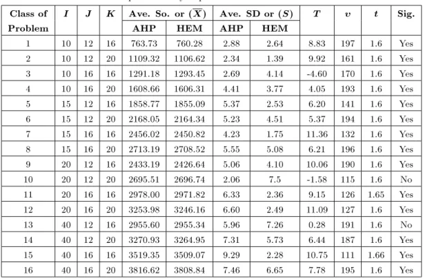
Now, for a more detailed comparison, two al-gorithms of HEM and an integrated approach of the analytical hierarchy process presented, or AHP by Xia and Wu [13] are considered. Care must be taken that in this paper suppliers do not oer price discounts on total business volume.
The test problems in this section were randomly generated based on combinations of the following pa-rameters.
1. I is equal to 10, 15, 20 or 40, 2. J is equal to 12 or 16, 3. K is equal to 16 or 20,
4. Dik is uniformly distributed over [100, 300],
5. Pij is uniformly distributed over [0.01, 0.05],
6. P is uniformly distributed over [0.90, 0.98]. A total of 1600 (4 2 2 100) test problems were generated. There are 100 test problems for each com-bination. Also, the stopping criterion is based on an elapsed CPU time given by (IJ) seconds. We test the hypothesis that the population corresponding to the
Table 1. Computational results for the algorithm.
I = 10 I = 15 I = 20 I = 40 J
K 2 4 8 12 16 2 4 8 12 16 2 4 8 12 16 2 4 8 12 16 Ave. 1 1.48 1.56 1.59 1.62 1.81 1.58 1.69 1.97 2.04 2.21 1.64 1.79 1.99 2.26 2.44 1.76 1.92 1.95 2.02 2.07 1.87 2 1.56 1.69 1.61 1.65 1.92 1.72 1.83 2.02 2.14 2.28 1.68 1.87 2.01 2.43 2.61 1.85 2.08 2.08 2.09 2.12 1.96 4 1.64 1.85 1.91 1.96 2.00 1.84 1.85 2.35 2.17 2.47 1.86 1.87 2.25 2.50 2.86 2.04 2.50 2.19 2.22 2.45 2.14 8 2.01 2.53 2.83 2.35 2.91 1.93 2.73 3.27 2.82 3.26 2.62 2.66 2.77 3.03 4.03 2.99 3.52 2.88 2.38 3.10 2.83 12 2.54 3.50 3.43 2.76 3.17 2.48 3.92 4.18 3.79 4.32 3.35 2.82 3.99 4.43 4.63 3.13 4.03 3.97 2.71 4.62 3.59 16 3.69 3.50 4.92 3.13 4.73 3.31 4.62 4.47 4.59 5.65 3.94 3.78 5.94 5.31 6.33 4.63 5.86 5.81 2.98 6.42 4.68 20 4.27 4.40 5.42 3.18 6.95 4.39 5.50 5.56 6.72 7.74 4.03 4.59 7.27 5.93 8.29 6.03 7.90 6.23 3.09 8.04 5.78 Ave. 2.46 2.72 3.10 2.38 3.36 2.46 3.16 3.40 3.47 3.99 2.74 2.77 3.75 3.70 4.46 3.20 3.97 3.59 2.50 4.12 3.26
dierences has a mean of zero. Specically, we test the (null) hypothesis, = 0, against the alternative, > 0. We assume that the solution dierence is a Normal variable, and choose the signicance level, = 0:05. If the hypothesis is true, random variable T = (X1 X2)=p(S12=n1) + (S22=n2) has a t distribution
with: = (S2
1=n1 + S22=n2)2=
(S2 1=n1)2
n1 1 +
(S2 2=n2)2
n2 1
degrees of freedom. The critical value of c is obtained from the relation Prob (T > c) = = 0:05. For example, the rst entry in Table 2 corresponds to the sample size = n1 = n2 = 100, 0 = 0: Sample mean
for HEM and AHP are X1= 760:28 and X2= 763:73,
respectively. The sample standard deviation for HEM and AHP are S1 = 2:64 and S2 = 2:88, respectively.
Since t = 1:6 < T = 8:83, we conclude that the dierence is statistically signicant. Table 2 displays that HEM outperforms AHP in all cases except two classes of problem (Classes 3 and 10), one of them being signicant (Class 3). Also, in cases where HEM yields better results, all dierences are signicant except one class (Class 13). In fact, HEM outperforms AHP in 86 percent of cases and signicantly outperforms in 81 percent.
CONCLUSION
Supplier selection is a multi-criteria decision making problem, which includes both qualitative and
quanti-tative factors. In order to select the best suppliers, it is necessary to make a trade-o between these tangible and intangible factors, some of which may conict. This paper considered a new theory in the supplier selection area and also presented a new algorithm for the supplier selection problem. The proposed problem in the supplier selection area is dened based on a real world situation. The idea behind the denition of this problem is the presentation of a new vision regarding the selection of some good suppliers and, also, consideration of some good and eective criteria in decision making and nally, a conceptually simple solution technique that is practically motivated and easily implemented for the supplier selection problem. The developed model is compatible when considering all costs imposed onto the production section for the sake of selection; a special supplier that managers face in the real world. Solving the model takes a lot of time, and since mathematical models are unable to render optimal solutions for large scale problems, it justies the utilization of meta-heuristics. Therefore, to solve the problem in proper time and, also, with a good qual-ity of solution, we introduce a novel Electromagnetism-like algorithm. Experimental results demonstrate that the proposed algorithm nds solutions from 1.04 to 1.08 of the lower bounds or within 1.03 of them, on average, and, hence, is quite satisfactory. Also, computational results demonstrate the performance of our algorithm compared to some of the strong algorithms recently
Table 2. Comparison study of performance between HEM and AHP.
Class of I J K Ave. So. or (X) Ave. SD or (S) T t Sig. Problem AHP HEM AHP HEM
1 10 12 16 763.73 760.28 2.88 2.64 8.83 197 1.6 Yes 2 10 12 20 1109.32 1106.62 2.34 1.39 9.92 161 1.6 Yes 3 10 16 16 1291.18 1293.45 2.69 4.14 -4.60 170 1.6 Yes 4 10 16 20 1608.66 1606.31 4.41 3.77 4.05 193 1.6 Yes 5 15 12 16 1858.77 1855.09 5.37 2.53 6.20 141 1.6 Yes 6 15 12 20 2168.05 2164.34 5.23 4.51 5.37 194 1.6 Yes 7 15 16 16 2456.02 2450.82 4.23 1.75 11.36 132 1.6 Yes 8 15 16 20 2713.19 2708.52 5.55 5.08 6.21 196 1.6 Yes 9 20 12 16 2433.19 2426.64 5.06 4.10 10.06 190 1.6 Yes 10 20 12 20 2695.51 2696.74 2.06 7.5 -1.58 115 1.6 No 11 20 16 16 2978.00 2971.82 6.33 2.36 9.15 126 1.65 Yes 12 20 16 20 3253.98 3246.16 6.60 2.49 11.09 127 1.6 Yes 13 40 12 16 2955.60 2955.34 5.96 7.26 0.28 191 1.6 No 14 40 12 20 3270.93 3264.95 7.31 5.73 6.44 187 1.6 Yes 15 40 16 16 3519.35 3509.07 9.29 2.28 10.75 111 1.66 Yes 16 40 16 20 3816.62 3808.84 7.46 6.65 7.78 195 1.6 Yes
Ins: Instance no.; Ave.: Average; So.: Solution; SD: Standard Deviation; Sig: Signicant. Each instance contains 100 independent tests.
developed. It is noticeable that as far as the dierences between algorithms are concerned, most of them are also signicant at the level = 0:05.
REFERENCES
1. Baker, K.R., Elements of Sequencing and Scheduling, 1st Ed., Toronto, University of Toronto bookstores (1996).
2. Huang, S.H. and Keskar, H. \Comprehensive and con-gurable metrics for supplier selection", International Journal of Production Economics, 105(2), pp. 510-523 (2007).
3. Boer, L., Labro, E. and Morlacchi, P. \A review of methods supporting supplier selection", European Journal of Purchasing and Supply Management, 7(2), pp. 75-89 (2001).
4. Donaldson, B. \Supplier selection criteria on the ser-vice dimension, some empirical evidence", European Journal of Purchasing and Supply Management, 1(4), pp. 209-217 (1994).
5. Weber, C.A., Current, J.R. and Benton, W.C. \Vendor selection criteria and methods", European Journal of Operational Research, 50, pp. 2-18 (1991).
6. Ghodsypour, S.H. and O'Brien, C. \Decision sup-port system for supplier selection using an integrated analytic hierarchy process and linear programming", International Journal of Production Economics, 56(1), pp. 199-212 (1998).
7. Liao, Z. and Rittscher, J. \A multi-objective sup-plier selection model under stochastic demand con-ditions", International Journal of Production Eco-nomics, 105(1), pp. 150-159 (2007).
8. Katsikeas, C.S., Paparoidamis, N.G. and Katsikea, E. \Supply source selection criteria: The impact of supplier performance on distributor performance", Industrial Marketing Management, 33(8), pp. 755-764 (2004).
9. Kamann, D.F. and Bakker, E.F. \Changing supplier selection and relationship practices: A contagion pro-cess", Journal of Purchasing and Supply Management, 10(2), pp. 55-64 (2004).
10. Ghodsypour, S.H. and O'Brien, C. \The total cost of logistics in supplier selection, under conditions of multiple sourcing, multiple criteria and capacity constraint", International Journal of Production Eco-nomics, 73(1), pp. 15-27 (2001).
11. Boer, L., Wegen, L. and Telgen, J. \Outranking methods in support of supplier selection", European Journal of Purchasing and Supply Management, 4(2-3), pp. 109-118 (1998).
12. Houshyar, A. and Lyth, D. \A systematic supplier selection procedure", Computers and Industrial Engi-neering, 23(1-4), pp. 173-176 (1992).
13. Xia, W. and Wu, Z. \Supplier selection with multiple criteria in volume discount environments", Omega, 35(5), pp. 494-504 (2007).
14. Banker, R.D. and Khosla, I.S. \Economics of opera-tions management: A research perspective", Journal of Operations Management, 12, pp. 423-425 (1995). 15. Verma, R. and Pullman, M.E. \An analysis of the
supplier selection process", Omega, 26(6), pp. 739-750 (1998).
16. Jayaraman, V., Srivastava, R. and Benton, W.C. \Supplier selection and order quantity allocation: A comprehensive model", The Journal of Supply Chain Management, 35, pp. 50-58 (1999).
17. Wang, H.S. and Che, Z.H. \An integrated model for supplier selection decisions in conguration changes", Expert Systems with Applications, 32(4), pp. 1132-1140 (2007).
18. Lopez, R.F. \Strategic supplier selection in the added-value perspective: A CI approach", Information Sci-ences, 177(5), pp. 1169-1179 (2007).
19. Choi, J.H. and Chang, Y.S. \A two-phased semantic optimization modeling approach on supplier selection in e-procurement", Expert Systems with Applications, 31(1), pp. 137-144 (2006).
20. Hang, G., Park, S.C., Jang, D.S. and Rho, H.M. \An eective supplier selection method for constructing a competitive supply-relationship", Expert Systems with Applications, 28(4), pp. 629-639 (2005).
21. Benton, W.C. and Whybark, D.C. \Material require-ments planning (MRP) and purchase discounts", Jour-nal of Operations Management, 2, pp. 137-143 (1982). 22. Hariga, M. and Haouari, M. \An EOQ lot sizing model with random supplier capacity", International Journal of Production Economics, 58, pp. 39-47 (1999). 23. Rosenthal, E.C., Zydiak, J.L. and Chaudhry, S.S.
\Vendor selection with bundling", Decision Sciences, 26, pp. 35-48 (1995).
24. Basnet, C. and Leung, M.Y. \Inventory lot-sizing with supplier selection", Computers and Operations Research, 32(1), pp. 1-14 (2005).
25. Degraeve, Z., Labro, E. and Roodhooft, F. \An evaluation of vendor selection models from a total cost of ownership perspective", European Journal of Operational Research, 125(1), pp. 34-58 (2000). 26. Debels, D., De Reyck, B., Leus, R. and Vanhoucke,
M. \A hybrid scatter search/electromagnetism meta-heuristic for project scheduling", European Journal of Operational Research, 169(2), pp. 638-653 (2006). 27. Chang, P.C., Chen, S.S. and Fan, C.Y. \A hybrid
electromagnetism-like algorithm for single machine scheduling problem", Expert Systems with Applica-tions, 36, pp. 1259-1267 (2009).
28. Gupta, S.R. and Smith, J.S. \Algorithms for sin-gle machine total tardiness scheduling with sequence dependent setups", European Journal of Operational Research, 175, pp. 722-739 (2006).
BIOGRAPHIES
Mohammad Mirabi was born in Yazd, Iran, on December 16th, 1979. He received his MS and PhD degrees in Industrial Engineering from Amirkabir University of Technology, Tehran in 2003 and 2008, respectively. His research and teaching interests in-clude: Project Management, Production Management, Flowshop Scheduling and Economics.
Seyyed Mohammad Taghi Fatemi Ghomi was born in Ghom, Iran on March 11th, 1952. He received his BS degree in Industrial Engineering from Sharif University of Technology, Tehran, in 1973, and his PhD degree in Industrial Engineering from Bradford University, England, in 1980. He is currently a Professor in the Department of Industrial Engineering
at Amirkabir University of Technology in Tehran. His research and teaching interests include: Stochastic Activity Networks, Production Planning and Control, Scheduling, Queuing Systems, and Statistical Quality Control.
Fariborz Jolai was born in Tehran, Iran, on July 27th, 1965. He received his BS and MS degrees in Industrial Engineering from Amirkabir University of Technology, Tehran, in 1986 and 1989, respectively. He also received his PhD from `Ecole National Superieure de Genie Industriel', at the `Institut National Polytech-nique de Grenoble' in France, in 1998. He is currently an Associate Professor in the College of Engineering at the University of Tehran. His research interests include: Scheduling, Plant Layout, and Stochastic Activity Networks.