Sharif University of Technology
Scientia IranicaTransactions E: Industrial Engineering www.scientiairanica.com
A computational approach to economic production
quantity model for perishable products with
backordering shortage and stock-dependent demand
H. Mokhtari
a;, A. Naimi-Sadigh
band A. Salmasnia
ca. Department of Industrial Engineering, Faculty of Engineering, University of Kashan, Kashan, Iran. b. Iranian Research Institute for Information Science and Technology (IRANDOC), Tehran, Iran.
c. Department of Industrial Engineering, Faculty of Engineering and Technology, University of Qom, Qom, Iran. Received 9 April 2016; received in revised form 26 June 2016; accepted 25 July 2016
KEYWORDS Production-inventory; EPQ;
Stock-dependent demand; Grid search; Simulation-based optimization.
Abstract. This paper deals with an Economic Production Quantity (EPQ) model to determine production-inventory policies for perishable products. Shortage is permitted and fully backordered. The demand rate is stochastic- and stock-dependent. Since the problem is mathematically challenging and intractable via analytical approaches, this paper designs a simulation-based optimization algorithm by combining a grid search and a simulation model to solve the problem. The grid search plays the role of optimizer to determine the model variables, and the simulation model is utilized to evaluate the quality of solutions obtained by the optimizer through an iterative procedure. Eventually, a numerical example is discussed to illustrate how the solution procedure works, and a comparison study is carried out to demonstrate the superiority of suggested approach. Moreover, a comprehensive sensitivity analysis with respect to the problem parameters is performed.
© 2017 Sharif University of Technology. All rights reserved.
1. Introduction
In today markets, the manufacturers are often encoun-tered with high degrees of competition forcing them to improve their performance continuously. One of the main systems which greatly inuences the performance of manufacturers is inventory system. Raw materials, sparse parts, work in processes, and nished goods are various types of inventory. The important decision in an inventory system is how many and when a company should order goods. If inventories are not controlled appropriately, they might become unreliable, inecient, and costly. Since most companies in any
*. Corresponding author. Tel.: 031 55912476 E-mail addresses: mokhtari [email protected] (H. Mokhtari); [email protected] (A. Naimi-Sadigh); [email protected] (A. Salmasnia)
industrial sectors have some types of inventory, many studies have been conducted on dierent types of inventory systems so far. Although inventory problems are usually developed based on basic assumptions in earlier literature, they are still extensively employed by industries. The Economic Production Quantity (EPQ) model, also known as the Economic Manufacturing Quantity (EMQ), is one of the basic types of inventory model that determines the optimal production rate of an item for a facility. The aim of the EPQ model is of-ten to optimize the total inventory and production cost, when items are processed internally instead of being provided from external sources. In some recent studies on the EPQ, Pan et al. [1] developed an integrated EPQ model with the statistical process control and maintenance issues. Additionally, Wee et al. [2] devised an economic production quantity model and a renewal reward theorem-based procedure for imperfect items
with shortage and screening constraints. Dash et al. [3] proposed a deteriorating inventory model incorporating time-value of money with price-dependent demand and Discounted Cash Flows (DCF) approach. Karimi-Nasab and Sabri-Laghaie [4] designed an imperfect EPQ problem with random defectives, reworkable and non-reworkable items. Moreover, Nasr et al. [5] dis-cussed an EPQ model with deteriorating raw material and analyzed the model via dierential equations. Pacheco-Velazquez and Cardenas-Barron [6] analyzed an economic production quantity model by considering ordering and holding costs for both raw materials and nished products. Jawad et al. [7] developed an EPQ model based on the laws of thermodynamics focusing on the three pillars of sustainability and computed their costs. In addition, Sadeghi et al. [8] presented a multi-item economic production quantity model with fuzzy demand, backordering shortage, and limited space of warehouse. Al-Salamah [9] suggested an economic pro-duction quantity model for a case where the propro-duction process and inspection are both not perfect in order to nd the optimal lot size for batch manufacturing while the batches are subjected to destructive or non-destructive acceptance quality control process.
Many researchers presented their work on the EPQ model by considering dierent parameters such as setup cost, rework process, scrap goods, inspection, de-terioration, machine breakdown, backorder, shortage, etc. The majority of researchers on the EPQ models do not take into account the fact that customer behavior is not necessarily independent of system parameters. Traditional inventory models consider that the demand rate is constant [10], and some recent studies on the inventory models investigate the demand rate as a function of dierent variables such as price, advertise-ment, etc. [11-12]. However, all these models consider that the demand rate is independent of the inventory level. For certain types of products, the demand may be inuenced by the inventory level. It has been observed that neglecting the eect of inventory systems on customer's behavior leads to poor performance of the inventory management system. Thus, the inventory systems with some dependence between the system parameters have received the researchers' attention in recent years. In such a situation, an increase in the product space usually has a positive impact on the sales of that product. It is usually observed by practitioners that a large amount of goods displayed in a supermarket attracts more customers, and conversely, low inventory of goods might make the perception that they are not fresh, and therefore decreases the demand. Consequently, building up the inventory often has a positive impact on the sales and prots. Therefore, in such a case, the demand has no longer a constant rate, but it depends on the inventory level. This case is known as stock-dependent demand or
inventory-level-dependent demand in the inventory literature. As a result, many researchers have dedicated considerable attention to the inventory systems with a demand dependent on the stock level. Gupta and Vrat [13] were the rst researchers that introduced inventory models with stock-dependent demand rate. Later, Recently, Chang et al. [14] have considered an EOQ model with stock-dependent demand and obtained the optimal replenishment policy while maximizing the total prot. In addition, Yang et al. [15] discussed an inventory model under ination for stock-dependent consump-tion rate products with shortage. Shah et al. [16] derived optimal inventory policy for a price-sensitive and stock-dependent demand inventory system under a payment scheme. Sarkar and Sarkar [17] proposed an inventory model for deteriorating items with stock-dependent demand, time-varying backordering, and time-varying deterioration rate to determine the op-timal cycle length, such that the expected total cost is minimized. Soni [18] extended the previously proposed inventory model for deteriorating items under stock-dependent demand and two-level trade credit. Singh and Sharma [19] presented a mathematical model for an inventory problem with stock-dependent demand and deterioration to analyze the retailer's optimal in-ventory policy under the permissible delay in payment. Krommyda et al. [20] studied a substitutable inventory management system where the demand for each prod-uct depends on the inventory levels. Wu and Zhao [21] suggested an economic order quantity model for de-teriorating items with a current inventory-dependent and linearly increasing time-varying demand under trade credit. Tripathi and Singh [22] analyzed an inventory model with stock-dependent demand and dierent holding cost patterns. Tsoularis [23] consid-ered the prot maximization inventory problem with the demand varied by price and stock availability. Chakraborty et al. [24] discussed multi-item integrated production-inventory models with stock-dependent de-mand and nonlinear cost functions. Recently, Palanivel and Uthayakumar [25] discussed an economic ordering quantity model with stock-dependent demand and imperfect products under the eect of ination and time value of money.
Almost all physical items deteriorate over time, and the deterioration of physical goods cannot be dis-regarded. Consequently, a major issue of the inventory system in a business organization is the maintenance of perishable products inventories. Since deterioration often leads to decreasing the usefulness of the items over time, the deterioration is a major parameter in de-signing inventory systems. In such a case, deterioration is dened as decay, damage, spoilage, evaporation or loss of the marginal value of goods. The examples are drugs, volatile liquids, blood, vegetables, fruits, food products, photographic lms, pharmaceuticals,
chemi-cals, electronic goods, and radioactive substances. As a result, the inventory problem of perishable items has been studied by researchers. The work done by Ghare and Schrader [26] was the rst attempt to design an optimal inventory system for perishable products where an inventory model with an exponentially deteriorating inventory was discussed. Afterwards, a comprehensive review of perishable literature till 2011 was provided by Goyal and Giri [27]. Later, Balkhi [28] discussed an inventory model for perishable products under supplier trade credits case considering time value of money. Bansal [29] developed the inventory model for deteriorating items under ination. Vahdani et al. [30] discussed a single-item lot-sizing and scheduling problem with deteriorating inventory over time and multiple warehouses. Later, Bhaula and Kumar [31] provided an optimal inventory policy for two-parameter Weibull deterioration. Recently, Giri and Sharma [32] provided an integrated inventory model for a perish-able item under allowperish-able shortages and credit linked wholesale price assumptions. Li et al. [33] studied an EPQ model considering both product deterioration and deteriorating production system with rework. Jaggi, et al. [34] considered a two-warehouse manufacturing inventory model for deteriorating items with imperfect quality under permissible delay in payments to maxi-mize the total prot per unit time. Moreover, Kouki et al. [35] modeled a coordinated inventory system for perishable items with random lifetime and positive lead time as a Markov process. Moreover, Teimoury and Kazemi [36] presented a two-stage supply chain, including a wholesaler and a retailer, which produces a single deteriorating product with a constant rate.
One of the factors that increases the complexity of the inventory systems is the uncertainty existing in the parameters and the input data. Numerous researchers have developed inventory models with stochastic de-mand functions. For example, Timmer et al. [37] analyzed the cooperation strategies for the continuous review inventory systems with Poisson demand. Juan et al. [38] designed a simheuristic algorithm by combin-ing simulation and heuristics for solvcombin-ing a stochastic inventory problem considering distribution. Besides, Bieda [39] investigated an application of the stochastic approach to life cycle inventory data for a real case in Poland. Recently, Tamjidzad and Mirmohammadi [40] have discussed a single-item inventory system with resource constraint and quantity discount while consid-ering stochastic demand. In addition, Wu et al. [41] proposed a supply chain problem of the coordination policy under vendor-managed consignment inventory subject to consumer return and stochastic demand. Purohit et al. [42] discussed an inventory lot-sizing and supplier selection problem considering time-varying stochastic demand. Chuang et al. [43] evaluated some models with stochastic ramp-type demand in the
literature. In the current paper, in order to make the problem closer to real-world conditions, we assume a stochastic demand function.
In this paper, an appropriate production-inventory policy model based on a stochastic EPQ for a perishable product with tock-dependent demand is studied. It is assumed that shortages are allowed for the product and fully backordered. The main objective is to determine the optimal inventory cycle time and production quantity. The rest of this paper is organized as follows. Section 2 presents the notations and assumptions. The mathematical model is constructed in Section 3 while the solution algorithm is designed in Section 4. Section 5 discusses the experimental results. Finally, Section 6 concludes the paper.
2. Model notations and assumptions
The following notations are employed throughout the paper:
P Production rate per unit time Deterioration rate per unit time c Production cost per unit
h Holding cost per unit per unit time b Shortage cost per unit per unit time R Setup cost per cycle
k Selling price per unit S Shortage per cycle D(t) Demand rate at time t
" Stochastic term of the demand function I(t) Inventory level at time t
A Constant term of the stock-dependent demand rate
B Coecient of the inventory level in the stock-dependent demand function Imax Maximum inventory level
t0 Starting time of the planning horizon
when the maximum shortage occurs t1 The time when inventory becomes zero
for the rst time per cycle
t2 The time in which inventory reaches to
its maximum level
t3 The time when inventory becomes zero
for the second time per cycle T Inventory cycle time
I1(t) Inventory level at time interval [t0; t1]
I2(t) Inventory level at time interval [t1; t2]
I3(t) Inventory level at time interval [t2; t3]
I4(t) Inventory level at time interval
[t3; T + t0]
The proposed model in this paper is developed based on the following assumptions:
1. The production-inventory system involves a single product;
2. The demand rate is sensitive to the stock level when I(t) 0;
3. The production rate is nite and constant;
4. The lead time is assumed to be zero;
5. Deterioration process occurs as soon as a product is produced;
6. Deterioration rate is constant over the time period;
7. There is no replacement or repair for deteriorating products over the time period and the deteriorated products are removed from the system immediately;
8. Shortages are allowed and fully backordered;
9. Setup cost is incurred per cycle;
10. Holding cost is only applied to the product units;
11. The demand function is stochastic.
3. Model formulation
The behavior of the production-inventory model is de-picted by Figure 1. According to this model, the inven-tory system could be divided in four intervals. During time interval [t0; t1], the inventory level increases due
to the fact that the production rate is higher than the demand rate. At this interval, the demand rate is equal to constant A due to negative inventory level. Subsequently, on interval [t1; t2], the inventory level
continues to increase because the production rate is higher than the demand rate and the deterioration occurs until the inventory level reaches the maximum level Imax. The demand rate is dependent on the
stock A + BI(t) at this interval. During the next time interval [t2; t3], the inventory level decreases owing to
the demand and deterioration rates till the inventory level becomes zero at time t3. Finally, a shortage
occurs as the demand grows only during time interval [t3; T + t0]. The shortage continues up to the end of
the current inventory cycle.
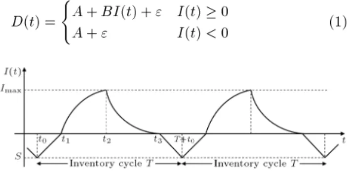
The demand function is considered as follows:
D(t) = (
A + BI(t) + " I(t) 0
A + " I(t) < 0 (1)
Figure 1. Inventory level illustration.
where " represents the stochastic term of the demand function. It means that demand function, D(t), is a stochastic variable with the expected value E[D(t)]:
E[D(t)] = (
A + BI(t) I(t) 0 A I(t) < 0
and random term ". Without loss of generality, let us assume that t0 = 0 and I1(t) indicates the inventory
level at time t (0 t t1), then we have:
dI1(t)
dt = P D(t) = P A 0 t t1: (2) With boundary condition I1(t1) = 0, it is concluded
that:
I1(t) = (P A)(t t1) 0 t t1: (3)
As it is obvious from Figure 1, I1(0) = S; hence, it
can be obtained that:
S = (P A)t1: (4)
Assume that I2(t) represents the inventory level at time
t (t1 t t2), then we have:
dI2(t)
dt + I2(t) = P D(t) t1 t t2: (5) Considering D(t) = A + BI(t) for t1 t t2 and
boundary condition I2(t1) = 0, it is concluded that:
I2(t)=
P A
+B h
1 e(+B)(t1 t)i t
1 t t2: (6)
Let I3(t) represent the inventory level at time t (t2
t t3), then it is concluded that:
dI3(t)
dt + I2(t) = D(t) t2 t t3: (7) Considering D(t) = A + BI(t) for t2 t t3with the
boundary condition I3(t3) = 0:
I3(t) = ( + B)A
h
e(+b)(t3 t) 1i t
2 t t3: (8)
It is obvious from Figure 1 that I2(t2) = I3(t2) = Imax;
therefore, we can obtain t2 in terms of t1 and t3 as
follows:
t2=( + B)1 log
P
Ae(+B)t3+(P A)e(+B)t1
: (9)
By substituting t2into I2(t) or I3(t), maximum
inven-tory level Imax can be calculated in terms of t1 and t3
as follows:
Imax=A(P(+B)A)
e(+B)t3 e(+B)t1
Ae(+B)t3+(P A)e(+B)t1
:(10)
Assume that I4(t) represents the inventory level at time
t (t3 t T ), then we have:
dI4(t)
dt = D(t) = A t3 t t4: (11) With boundary condition I4(t3) = 0, it is concluded
that:
I4(t) = ( A)(t t3) t3 t T: (12)
It is obvious from Figure 1 that I1(0) = I4(T ) = S;
therefore, we can obtain T in terms of t1 and t3 as
follows: T = t3+
P A
A
t1: (13)
Since the production is carried out in interval [0; t2]
with rate P , production quantity per cycle Q is given by P t2. Substituting t2into Q, it (t2) can be calculated
in terms of t1 and t3. Therefore, all of the required
information, including I1(t), I2(t), I3(t), I4(t), Imax,
S, and Q, are calculated in terms of t1 and t3. Hence,
we can form the total prot in terms of t1 and t3 as
follows:
(i) Setup cost per cycle R
(ii) Production Cost (PC):
P C = cP t2: (14)
Substituting t2 into PC, it is concluded that:
PC =( + B)cP log
P
Ae(+B)t3+ (P A)e(+B)t1
: (15)
(iii) Inventory Holding Cost (HC): HC = h
Z t2
t1
I2(t)dt +
Z t3
t2
I3(t)dt
= ( + B)h 2
Ae(+B)(t3 t2) 1
A( + B)(t3 t2)
+ (P A)( + B)(t2 t1)
+ (P A)e (+B)(t2 t1) 1: (16)
Substituting t2 into HC, the holding cost can be
rewritten in terms of t1 and t3as shown in Box I.
(iv) Shortage Cost (SC):
SC = b Z t1
0 [ I1(t)] dt +
Z T
t3
[ I4(t)] dt
= P bt21(P A)
2A : (18)
(v) Sales Revenue (SR) is calculated based on the dierence between the quantity of products pro-duced per cycle and the quantity of products deteriorated per cycle:
SR =k
Q
Z t2
t1
I2(t)dt +
Z t3
t2
I3(t)dt
1 ( + B)2
(A P )
e(+B)(t1 t2)
(t1 t2) 1
B(A P )(t1 t2)
A
e(+B)(t3 t2)+ t
2 At3 1
+ AB(t3 t2)
+ P kt2: (19)
Substituting t2 into SR, it yields:
SR =( + B)k 2
A(t3 t1) + P t1
P B log
P
Ae(+B)t3+ (P A)e(+B)t1
AB (t3+ (P 1)t1)
: (20)
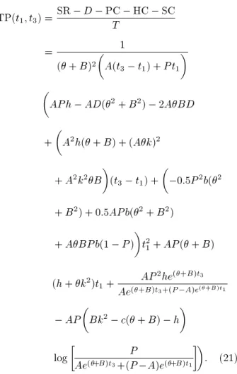
Hence, the total prot per time unit can be written as a function of t1 and t3 as follows:
HC = P h log h
P
Ae(+B)t3+(P A)e(+B)t1 i
+ A(t3 t1) + ABh(t3 t1) + P ht1( + B)
( + B)2 : (17)
TP(t1; t3) =SR D PC HC SCT
= 1
( + B)2
A(t3 t1) + P t1
AP h AD(2+ B2) 2ABD
+
A2h( + B) + (Ak)2
+ A2k2B(t
3 t1) +
0:5P2b(2
+ B2) + 0:5AP b(2+ B2)
+ ABP b(1 P )
t2
1+ AP ( + B)
(h + k2)t
1+ AP
2he(+B)t3
Ae(+B)t3+(P A)e(+B)t1
AP
Bk2 c( + B) h
log
P
Ae(+B)t3+(P A)e(+B)t1
: (21) This random demand function is utilized within all of the above equations. Hence, the total prot (Eq. (21)) has also a stochastic term because the demand function appears in its formulation. According to the above expressions, the problem can be formulated as a non-linear optimization model with a stochastic demand function as follows:
Maximize TP(t1; t3)
s.t.
t3 t1 t1; t3 0 (22)
4. Solution algorithm
A deep investigation into the problem formulated in the previous section reveals that it is rarely possible to obtain optimal production and inventory policies analytically. Additionally, the stochastic term of the demand function makes the problem more intractable. Therefore, we propose a computational approach as a simulation-based optimization algorithm to solve the problem. The simulation part is responsible for handling the uncertainty existing in the problem and evaluating the tness function. In order to achieve the global optimal solution, a simulator is combined with an optimizer. The optimizer is utilized to nd
Figure 2. The solution algorithm owchart.
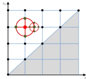
the best set of the solutions, and then the simulation is used to evaluate the quality of the generated solutions and guide the search movements. The optimization part in the proposed simulation-based optimization approach aims to calculate the values of the decision variables. Our proposed approach considers a grid search as an optimizer. It rst recognizes a feasible region with an equally divided grid, and then nds the best local solutions in that region. After that, it investigates the space around each local solution. During the search procedure, the algorithm may shift between spaces so as to nd better solutions. Briey, the algorithm consists of three main parts: (i) The initializing procedure; (ii) The neighborhood search process; and (iii) The simulation-based evaluation. Figure 2 presents a general procedure of the proposed approach.
4.1. Initializing procedure
The algorithm is initialized by selecting a divider factor, , which is a real value. The grid network in our problem has two axes: t1 and t3. Figure 3
shows the structure of grid network in our problem.
Figure 4. Inventory level for the case with t1= 0 and
t3> 0.
The factor divides the axes of the grid network equally, and then creates the points by marking intersections of the horizontal and vertical grid lines. Figure 2 illustrates a grid network whose axes are divided by divider factor = 2. The algorithm recognizes the points that are feasible subject to constraint t3 t1.
Figure 3 shows the feasible region of the grid network for the current problem. The set of feasible solutions is marked by the small dots in this gure. After that, all the feasible solutions in the grid network are evaluated by the simulator, and the tness values are estimated. Here, we can identify the local optimal solutions by nding the points with greater tness values among their neighbors. In Figure 3, the arrows show the directions where the tness value of the feasible solutions increases. The local optimal solutions found so far are depicted by large dots in the grid network of Figure 3. These solutions are utilized as the initial solutions for the neighborhood search process. To this end, the smaller grid is formed around the local optimal solutions to further investigate the solution space.
For further analysis of the grid network, we consider two extreme cases in the solution space. Let us rst consider a case in which t1= 0 and t3> 0. On
the grid network, the corresponding point of this case lies on the vertical axes. In such a case, we have no shortage during the inventory cycle, and hence t1= t0
and t3= T . This case occurs when the shortage cost is
much greater than other cost parameters in the model. Figure 4 depicts the inventory curve for the rst case.
As another extreme case, assume that t1 = t3
with a value greater than zero. It means that we have no holding cost during the inventory cycle. On the grid network, the corresponding points of this case lie on 45-degree line. This case occurs when the holding cost is much greater than other cost parameters in the model. Figure 5 depicts the inventory curve for the second case.
4.2. Neighborhood search process
As described in the previous section, the simulation-based optimization initializes the local optimal solution and feeds it into the neighborhood search process as a starting point. Indeed, for each local solution, the algorithm utilizes the neighborhood search procedure and updates the best solution through an iterative
Figure 5. Inventory level for the case with t1= t3.
Figure 6. The neighborhood search process.
search procedure. For this purpose, neighborhood grids are established around each solution to search for better solutions. A neighborhood grid is a smaller grid network inside the master grid network whose center is placed on the current solution and includes new points on the interstitial points between the points around the current solution. As an example, Figure 6 shows a neighborhood grid. The green circles show new points found on the grid network to be further investigated. These interstitial green points are obtained by adding =(2Iter) to the current solution where Iter represents the total number of iterations. Whenever the current solution is replaced by a new better solution, a neigh-borhood grid is established around the new solution. If there is no better solution than the current one on the neighborhood grid, a new narrower neighborhood grid is established around the current solution for further investigation.
4.3. Evaluation by simulation
This step uses simulation to estimate the total prot of a given set of solutions. As mentioned before, the complicated relationships and the uncertainty existing in the problem make it dicult to achieve the total prot via an analytical approach. In such a situa-tion, simulation can reasonably estimate the objective function for each solution in the grid network and evaluate the quality of the solutions generated by the
Figure 7. The simulation-based optimization procedure.
grid search. The simulation experiments are con-ducted several times. In each experiment, the demand function is randomly generated from the associated distribution and the total prot is estimated for the current solution. This brings about the conversion of the problem into a special deterministic one at each iteration. After all the experiments are implemented, the expected value of the total prot is calculated as the average amount of the special total prots estimated. Figure 7 depicts a general scheme of the simulation-based optimization procedure.
5. Experimental results
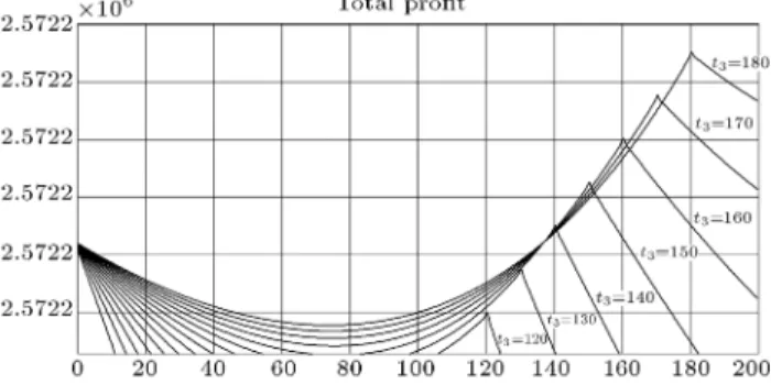
This section aims at discussing some experiments that have been carried out to investigate the performance of the proposed approach for the production-inventory problem. As mentioned earlier, it is rarely possible to analytically solve the current production-inventory problem for perishable products with shortage and stochastic stock-dependent demands. For further anal-ysis, the shape of TP function is investigated for an instance problem. Figures 8 and 9 show the behavior of TP in terms of variables t1 and t3. These gures
reveal that the Total Prot, TP, is neither concave nor convex globally. Moreover, as can be seen, it is not dierentiable in some potentially optimal points, which makes the problem more intractable.
5.1. A numerical example
In this sub-section, we aim at presenting a numerical
Figure 8. The total prot surface in terms of t1 and t3.
Figure 9. The total prot plot in terms of t1 and t3.
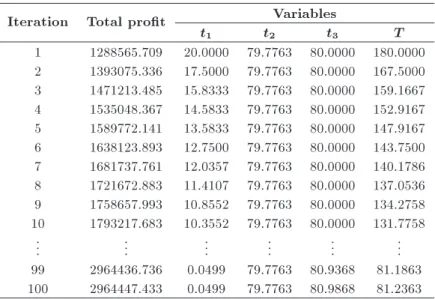
example in order to illustrate the procedure of the suggested approach step by step. The data considered in this example are as follows: production rate, P = 300; constant term of the demand function, A = 50; variable term of demand function, B = 8; deterioration rate, = 0:01; selling price, k = 100; holding cost, h = 2; shortage cost, b = 20; production cost, c = 50; setup cost, R = 300; and " follows the standard normal distribution, N(0; 1). To construct the mathematical model for this example, the inventory levels at cycle T are obtained by substituting the above values. Then, to implement the simulation-based grid search, the inventory levels are used to compute the total prot function. The results of experiments for divider factor = 10; 25; 40; 60 are shown by Tables 1-4 . As can be seen, increasing divider factor leads to increasing the total prot for a xed number of iterations (Iter = 100) in this example. The best obtained solution is t1 = 0:0000, t3 = 87:9802 with TP = 2974233.2264
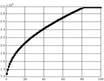
which is resulted from the algorithm with divider factor = 60. Moreover, Figures 10-13 show the convergence curves of the algorithm with dierent divider factors. As shown by these gures, the convergence behavior of the algorithm with the divider factor = 60 is outstandingly faster than other values.
5.2. Sensitivity analysis
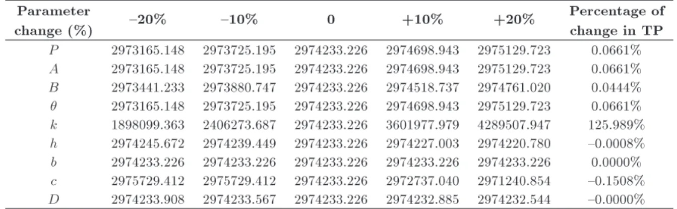
This subsection aims at performing a sensitivity analysis on the various parameters using the numerical example discussed in the previous subsection. We set divider factor at = 60 in this subsection. The results of analysis are presented in Table 5.
The output of the system considered here is the Total Prot, TP. The last column calculates the range of variations for the total prot by changing the parameters from {20% to +20%. As the results show, the total prot is less sensitive to changes in h, b, and D. It is moderately sensitive to changes in P; A; B; , and c, and highly sensitive to changes in k. Moreover, it reveals that there is an increase in the Total Prot, TP, value when P; A; B; , and k increase, and there is an increase in the Total Prot, TP, value when h, c, and D decrease.
Table 1. Results with divider factor, = 10.
Iteration Total prot Variables
t1 t2 t3 T
1 1288565.709 20.0000 79.7763 80.0000 180.0000 2 1393075.336 17.5000 79.7763 80.0000 167.5000 3 1471213.485 15.8333 79.7763 80.0000 159.1667 4 1535048.367 14.5833 79.7763 80.0000 152.9167 5 1589772.141 13.5833 79.7763 80.0000 147.9167 6 1638123.893 12.7500 79.7763 80.0000 143.7500 7 1681737.761 12.0357 79.7763 80.0000 140.1786 8 1721672.883 11.4107 79.7763 80.0000 137.0536 9 1758657.993 10.8552 79.7763 80.0000 134.2758 10 1793217.683 10.3552 79.7763 80.0000 131.7758
..
. ... ... ... ... ...
99 2964436.736 0.0499 79.7763 80.9368 81.1863 100 2964447.433 0.0499 79.7763 80.9868 81.2363
Table 2. Results with divider factor = 25.
Iteration Total prot Variables
t1 t2 t3 T
1 1604837.228 12.5000 74.7763 75.0000 137.5000 2 2093205.03 6.2500 74.7763 75.0000 106.2500 3 2609685.109 2.0833 74.7763 75.0000 85.4167 4 2622819.157 2.0833 77.9013 78.1250 88.5417 5 2632677.207 2.0833 80.4013 80.6250 91.0417 6 2640487.929 2.0833 82.4846 82.7083 93.1250 7 2921187.196 0.2976 82.4846 82.7083 84.1964 8 2922291.842 0.2976 84.0471 84.2708 85.7589 9 2923240.496 0.2976 85.4360 85.6597 87.1478 10 2924068.796 0.2976 86.6860 86.9097 88.3978
..
. ... ... ... ... ...
99 2973050.195 0.0069 87.5423 87.5697 87.8743 100 2973062.647 0.0069 87.5660 87.5847 87.9993
Table 3. Results with divider factor = 40.
Iteration Total prot Variables
t1 t2 t3 T
1 2186325.369 5.0000 69.7763 70.0000 95.0000 2 2238488.721 5.0000 76.4430 76.6667 101.6667 3 2973114.378 0.0000 76.4430 76.6667 76.6667 4 2973545.887 0.0000 80.4430 80.6667 80.6667 5 2973874.085 0.0000 83.7763 84.0000 84.0000 6 2974135.348 0.0000 86.6335 86.8571 86.8571 7 2973907.711 0.0000 84.1335 84.3571 84.3571 8 2974110.704 0.0000 86.3557 86.5794 86.5794 9 2973928.490 0.0000 79.7763 84.5794 84.5794 10 2973942.596 0.0000 86.1739 86.3975 86.3975
..
. ... ... ... ... ...
99 2974215.932 0.0000 87.5664 87.5880 87.7780 100 2974221.210 0.0000 87.6043 87.6080 87.9780
Table 4. Results with divider factor = 60.
Iteration Total prot Variables
t1 t2 t3 T
1 1091489.606 25.0000 29.7763 30.0000 155.0000 2 2959577.777 10.0000 29.7763 30.0000 80.0000 3 2964025.517 0.0000 29.7763 30.0000 30.0000 4 2966479.443 0.0000 37.2763 37.5000 37.5000 5 2968060.581 0.0000 43.2763 43.5000 43.5000 6 2969177.433 0.0000 48.2763 48.5000 48.5000 7 2970015.778 0.0000 52.5620 52.7857 52.7857 8 2970672.806 0.0000 56.3120 56.5357 56.5357 9 2971204.563 0.0000 59.6454 59.8690 59.8690 10 2971645.770 0.0000 62.6454 62.8690 62.8690
..
. ... ... ... ... ...
99 2974203.723 0.0000 86.6066 87.6272 87.8172 100 2974233.226 0.0000 86.5896 87.6402 87.9802
Figure 10. Convergence curve with divider factor = 10.
Figure 11. Convergence curve with divider factor = 25.
5.3. Comparisons
In order to investigate the quality of the solutions obtained by the suggested approach, the performances of a Genetic Algorithm (GA) and a full enumeration
Figure 12. Convergence curve with divider factor = 40.
Figure 13. Convergence curve with divider factor = 60.
algorithm are compared with our approach in this subsection. To this end, the GA structure is devised as follows. The chromosome is designed by a string with
Table 5. Sensitivity analysis results. Parameter
change (%) {20% {10% 0 +10% +20%
Percentage of change in TP P 2973165.148 2973725.195 2974233.226 2974698.943 2975129.723 0.0661% A 2973165.148 2973725.195 2974233.226 2974698.943 2975129.723 0.0661% B 2973441.233 2973880.747 2974233.226 2974518.737 2974761.020 0.0444% 2973165.148 2973725.195 2974233.226 2974698.943 2975129.723 0.0661% k 1898099.363 2406273.687 2974233.226 3601977.979 4289507.947 125.989% h 2974245.672 2974239.449 2974233.226 2974227.003 2974220.780 {0.0008% b 2974233.226 2974233.226 2974233.226 2974233.226 2974233.226 0.0000% c 2975729.412 2975729.412 2974233.226 2972737.040 2971240.854 {0.1508% D 2974233.908 2974233.567 2974233.226 2974232.885 2974232.544 {0.0000% Table 6. The result of comparisons among full enumeration, genetic algorithm, and grid search. Problem
no.
Selling price
(k)
Production cost
(c)
Full enumeration Genetic algorithm Grid search Grid size = 2 Grid size = 5 Grid size = 10
TP CPU
(s) TP
CPU
(s) TP
CPU
(s) TP
CPU
(s) TP CPU(s) 1 50 15 99398 206.14 99398 49.67 99398 26.34 99398 113.14 99398 55.29 2 30 106234 218.87 106200 52.19 106254 25.75 106232 112.41 106234 53.65 3 45 68726 207.80 68719 48.92 68702 25.05 68678 112.36 68726 53.84 4 60 780597 208.57 780430 48.56 780115 25.64 780044 112.25 780597 53.54 5 100 15 399398 205.12 399398 49.53 399398 25.24 399434 112.82 399408 52.79 6 30 598812 211.74 598823 49.87 598771 26.05 598652 112.63 598887 55.10 7 45 715025 231.49 714953 60.07 714834 27.57 714287 112.53 715034 54.07 8 60 1079243 216.11 1079100 49.10 1078935 25.67 1078965 113.08 1079251 55.41 9 150 15 966655 207.03 966620 52.55 966570 27.60 966414 112.50 966664 52.74 10 30 1780862 209.45 1780600 52.06 1780400 25.33 1779383 113.13 1780875 56.18 11 45 2445542 209.27 2445200 59.48 2444700 25.69 2443134 112.60 2445582 56.21 12 60 3407145 215.63 3406800 50.23 3406262 26.16 3404735 112.71 3407182 55.63 13 200 15 1823903 209.11 1823800 49.69 1823641 26.15 1823271 112.54 1823933 56.85 14 30 3435516 209.27 3435210 48.64 3434634 25.87 3432534 115.68 3436627 56.77 15 45 4868174 225.93 4867528 58.58 4866575 26.57 4864035 114.90 4868541 55.04 16 60 6666234 218.17 6665517 52.81 6664475 26.93 6659767 114.97 6666764 56.14 Average 1827592 213.11 1827394 52.00 1827104 26.10 1826185 113.14 1827731 54.95
two genes ft1; t3g. The initial population is produced
by assigning a random real number to each gene. The crossover operates on two parent solutions, P1 and P2,
in order to create new ospring solutions. For this purpose, a random number, 2 [0; 1], is generated and the osprings are obtained as P1+ (1 )P2 and
P2 + (1 )P1. The mutation alters the value of
the genes in order to make a random change to the solution. For this purpose, random binary number, , is generated and the mutation operator sets, t1 = 0,
if = 0, and t3 = t1; otherwise, the current solution
(t1; t3) is transmitted to the boundary of the feasible
region (t3 t1). For example, if we have (2.5,4.0)
as the current solution, mutation turns it to (0.0,4.0) if = 0, and to (2.5,2.5) if = 1. The standard
features of the GA algorithm used in this subsection are as follows: crossover rate = 0.3, mutation rate = 0.1, population size = 40, generation number = 300, and replication number = 5. In order to implement the algorithms, we need a wide range of test problems. To this end, we generate the instances using the uniform distribution. We categorize the instances based on selling price, k, and production cost, c, as the most sensitive parameters.
Table 6 summarizes the results of the comparison for the suggested grid search with the genetic algorithm and the full enumeration algorithm in terms of the Total Prot (TP) and the CPU time. Since the per-formance of the full enumeration algorithm is greatly dependent on the grid size, we examine three values for
the grid size f2; 5; 10g. As expected, among the three full enumeration algorithms, Grid size = 2 obtained better solutions than the two others. As the results presented in this table reveal, the suggested grid search algorithm obtains better solutions compared to both the full enumeration and genetic algorithms with less computational time.
6. Conclusions
As marketing researchers have recognized, the demand for many products is directly proportional to the amount of stock displayed. It is usually observed by the practitioners that a large amount of goods displayed in a supermarket attracts more customers, and conversely, low inventory of goods might make the perception that they are not fresh, and therefore decrease the demand. Consequently, building up the inventory level often has a positive impact on sales and prots. Therefore, in such a case, the demand has no longer a constant rate, but it depends on the stock level. Hence, this paper dealt with a stock-dependent demand for an EPQ model. The products are perishable and the shortage is permitted and fully backordered. In order to determine the appropriate production-inventory policies, the inventory level was formulated at dierent time horizons, and then the total prot function was derived. Since the problem is mathematically intractable, designing an analytical approach was a challenging task. Therefore, this paper developed a simulation-based optimization algorithm where a grid search was combined with a simulation model. The grid search plays the role of an optimizer to determine the values of the model variables, and the simulation model is utilized to evaluate the quality of the solutions obtained by the optimizer within an it-erative procedure. A numerical example was discussed and a sensitivity analysis was carried out with respect to the parameters of the model. The results showed that the total prot is highly sensitive to changes in k and moderately sensitive to changes in P; A; B; , and c. Moreover, the results of a comparison study demonstrate that the suggested approach is superior to genetic algorithm and full enumeration algorithms in terms of both accuracy and eciency features.
As for future study, it would be interesting to consider joint pricing and inventory policy. We also can extend the model by considering both stock- and price-dependent demand functions. As for another extension, the partial backordering can be investigated.
References
1. Pan, E., Jin, Y., Wang, S. and Cang, T. \An integrated EPQ model based on a control chart for an imperfect
production process", International Journal of Produc-tion Research, 50(23), pp. 6999-7011 (2012).
2. Wee, H.M., Wang, W.T. and Yang, P.C. \A production quantity model for imperfect quality items with short-age and screening constraint", International Journal of Production Research, 51(6), pp. 1869-1884 (2013).
3. Dash, B., Pattnaik, M. and Pattnaik, H. \Deterio-rated economic production quantity (EPQ) model for declined quadratic demand with time value of money and shortages", Applied Mathematical Sciences, 8(73), pp. 3607-3618 (2014).
4. Karimi-Nasab, M. and Sabri-Laghaie, K. \Develop-ing approximate algorithms for EPQ problem with process compressibility and random error in produc-tion/inspection", International Journal of Production Research, 52(8), pp. 2388-2421 (2014).
5. Nasr, W.W., Salameh, M.K. and Moussawi-Haidar, L. \Integrating the economic production model with de-teriorating raw material over multi-production cycles", International Journal of Production Research, 52(8), pp. 2477-2489 (2014).
6. Pacheco-Velazquez, E.A. and Cardenas-Barron, L.E. \An economic production quantity inventory model with backorders considering the raw material costs", Scientia Iranica, 23(2), pp. 736-746 (2016).
7. Jawad, H., Jaber, M.Y., Bonney, M. and Rosen, M.A. \Deriving an exergetic economic production quantity model for better sustainability", Applied Mathematical Modelling, 40(11-12), pp. 6026-6039 (2016).
8. Sadeghi, J., Akhavan Niaki, S.T., Malekian, M.R. and Sadeghi, S. \Optimising multi-item economic produc-tion quantity model with trapezoidal fuzzy demand and backordering: two tuned meta-heuristics", Euro-pean J. of Industrial Engineering, 10(2), pp. 170-195 (2016).
9. Al-Salamah, M. \Economic production quantity in batch manufacturing with imperfect quality, imperfect inspection, and destructive and non-destructive accep-tance sampling in a two-tier market", Computers & Industrial Engineering, 93(1), pp. 275-285 (2016).
10. Wang, S.-P. and Lee, W. \A note on A two-level supply chain with consignment stock agreement and stock-dependent demand", International Journal of Production Research, 54(9), pp. 2750-2756 (2016).
11. Naimi Sadigh, A., Chaharsooghi, S.K. and Sheikhmo-hammady, M. \A game theoretic approach to coordi-nation of pricing, advertising, and inventory decisions in a competitive supply chain", Journal of Industrial and Management Optimization, 12(1), pp. 337-355 (2016a).
12. Naimi Sadigh, A., Chaharsooghi, S.K. and Sheikhmo-hammady, M. \Game-theoretic analysis of coordinat-ing priccoordinat-ing and marketcoordinat-ing decisions in a multi-product multi-echelon supply chain", Scientia Iranica E, 23, pp. 1459-1473 (2016).
13. Gupta, R. and Vrat, P. \Inventory model with multi-items under constraint systems for stock dependent consumption rate", Operations Research, 24(1), pp. 41-42 (1986).
14. Chang, C.T., Teng, J.T. and Goyal, S.K. \Optimal replenishment policies for non-instantaneous deterio-rating items with stock-dependent demand", Interna-tional Journal of Production Economics, 123(1), pp. 62-68 (2010).
15. Yang, H.L., Teng, J.T. and Chern, M.S. \An in-ventory model under ination for deteriorating items with stock-dependent consumption rate and partial backlogging shortages", International Journal of Pro-duction Economics, 123(1), pp. 8-19 (2010).
16. Shah, N.H., Patel, A.R. and Lou, K.R. \Opti-mal ordering and pricing policy for price sensitive stock-dependent demand under progressive payment scheme", International Journal of Industrial Engineer-ing Computations, 2(3), pp. 523-532 (2011).
17. Sarkar, B. and Sarkar, S. \An improved inventory model with partial backlogging, time varying dete-rioration and stock-dependent demand", Economic Modelling, 30(1), pp. 924-932 (2013).
18. Soni, N.H. \Optimal replenishment policies for de-teriorating items with stock sensitive demand under two-level trade credit and limited capacity", Applied Mathematical Modelling, 37(8), pp. 5887-5895 (2013).
19. Singh, S.R. and Sharma, S. \Optimal trade-credit pol-icy for perishable items deeming imperfect production and stock dependent demand", International Journal of Industrial Engineering Computations, 5(1), pp. 151-168 (2014).
20. Krommyda, I.P., Skouri, K. and Konstantaras, I. \Op-timal ordering quantities for substitutable products with stock-dependent demand", Applied Mathematical Modelling, 39(1), pp. 147-164 (2015).
21. Wu, C.F. and Zhao, Q.H. \An inventory model for de-teriorating items with inventory-dependent and linear trend demand under trade credit", Scientia Iranica, 22(6), pp. 2558-2570 (2015).
22. Tripathi, R.P. and Singh, D. \Inventory model with stock dependent demand and dierent holding cost functions", International Journal of Industrial and Systems Engineering, 21(1), pp. 68-82 (2015).
23. Tsoularis, A. \An optimal inventory pricing and or-dering strategy subject to demand dependent on stock level and price", International Journal of Mathematics in Operational Research, 7(5), pp. 595-608 (2015).
24. Chakraborty, D., Kumar Jana, D. and Kumar Roy, T. \Multi-item integrated supply chain model for de-teriorating items with stock dependent demand under fuzzy random and bifuzzy environments", Computers & Industrial Engineering, 88(1), pp. 166-180 (2015).
25. Palanivel, M. and Uthayakumar, R. \An inventory model with imperfect items, stock dependent de-mand and permissible delay in payments under ina-tion", RAIRO-Operations Research, 50(3), pp. 473-489 (2016).
26. Ghare, P.M. and Schrader, G.H. \A model for ex-ponentially decaying inventory system", International Journal of Productions Research, 21(1), pp. 449-460 (1963).
27. Goyal, S.K. and Giri, B.C. \Recent trends in model-ing of deterioratmodel-ing inventory", European Journal of Operational Research, 134(1), pp. 1-16 (2001).
28. Balkhi, Z. \Optimal economic ordering policy with deteriorating items under dierent supplier trade cred-its for nite horizon case", International Journal of Production Economics, 133(1), pp. 216-223 (2011).
29. Bansal, K.K. \Inventory model for deteriorating items with the eect of ination", International Journal of Application and Innovation in Engineering and Management, 2(5), pp. 143-150 (2013).
30. Vahdani, M., Dolati, A. and Bashiri, M. \Single-item lot-sizing and scheduling problem with deteriorating inventory and multiple warehouses", Scientia Iranica, 20(6), pp. 2177-2187 (2013).
31. Bhaula, B. and Kumar, M.R. \An economic order quantity model for weibull deteriorating items with stock dependent consumption rate and shortages under ination", International Journal of Computing and Technology, 1(5), pp. 196-204 (2014).
32. Giri, B.C. and Sharma, S. \An integrated inventory model for a deteriorating item with allowable short-ages and credit linked wholesale price", Optimization Letters, 9(6), pp. 1149-1175 (2015).
33. Li, N., Chan, F.T.S., Chung, S.H. and Tai, A.H. \An EPQ model for deteriorating production system and items with rework", Mathematical Problems in Engineering, 957970 (2015).
34. Jaggi, C.K., Eduardo Cardenas-Barron, L., Tiwari, S. and Sha, A.A. \Two-warehouse inventory model for deteriorating items with imperfect quality under the conditions of permissible delay in payments", Scientia Iranica, 24, pp. 390-412 (2017).
35. Kouki, C., Zied Babai, M., Jemai, Z. and Minner, S. \A coordinated multi-item inventory system for per-ishables with random lifetime", International Journal of Production Economics, 181, pp. 226-237 (2016).
36. Teimoury, E. and Kazemi, S.M.M. \An integrated pricing and inventory model for deteriorating products in a two stage supply chain under replacement and shortage", Scientia Iranica, 24, pp. 342-354 (2017).
37. Timmer, J., Chess, M. and Boucherie, R.J. \Cooper-ation and game-theoretic cost alloc\Cooper-ation in stochastic
inventory models with continuous review", European Journal of Operational Research, 231(3), pp. 567-576 (2013).
38. Juan, A.A., Grasman, S.E., Caceres-Cruz, J. and Bektas, T. \A simheuristic algorithm for the single-period stochastic inventory-routing problem with stock-outs", Simulation Modelling Practice and The-ory, 46(1), pp. 40-52 (2014).
39. Bieda, B. \Application of stochastic approach based on Monte Carlo (MC) simulation for life cycle inventory (LCI) to the steel process chain: Case study", Science of the Total Environment, 481(1), pp. 649-655 (2014).
40. Tamjidzad, S. and Mirmohammadi, S.H. \An optimal (r, Q) policy in a stochastic inventory system with all-units quantity discount and limited sharable resource", European Journal of Operational Research, 247(1), pp. 93-100 (2015).
41. Wu, Z., Chen, D. and Yu, H. \Coordination of a supply chain with consumer return under vendor-managed consignment inventory and stochastic demand", Inter-national Journal of General Systems, 45(5), pp. 502-516 (2016).
42. Purohit, A.K., Choudhary, D. and Shankar, R. \In-ventory lot-sizing with supplier selection under non-stationary stochastic demand", International Journal of Production Research, 54(8), pp. 2459-2469 (2016).
43. Chuang, J.P.-C., Chou, W.-S. and Julianne, P. \In-ventory models with stochastic ramp type demand", Journal of Interdisciplinary Mathematics, 19(1), pp. 55-64 (2016).
Biographies
Hadi Mokhtari is currently an Assistant Professor of Industrial Engineering in University of Kashan, Iran.
His current research interests include the applications of operations research and articial intelligence tech-niques to the areas of project scheduling, production scheduling, and supply chain management. He also published several papers in international journals such as Computers and Operations Research, International Journal of Production Research, Applied Soft Com-puting, NeurocomCom-puting, International Journal of Ad-vanced Manufacturing Technology, IEEE Transactions on Engineering Management, Expert Systems with Applications and Scientia Iranica.
Ali Naimi-Sadigh is an Assistant Professor of In-dustrial Engineering in the Information Technology Management Faculty of the Iranian Research Institute for Information Science and Technology (IRANDOC). He received his BS, MS, and PhD degrees in In-dustrial Engineering from K.N. Toosi University of Technology, Amirkabir University of Technology, and Tarbiat Modares University, respectively. His research interests include pricing, supply chain, game theory, and optimization.
Ali Salmasnia is currently an Assistant Professor in University of Qom, Qom, Iran. His research interests include quality engineering, multi-response optimiza-tion, applied multivariate statistics, and multi-criterion decision making. He is the author or co-author of various papers published in Applied Soft Computing, Neurocomputing, IEEE Transactions on Engineering Management, International Journal of Advanced Man-ufacturing Technology, Applied Mathematical Mod-elling, Expert Systems with Applications, International Journal of Information Technology and Decision Mak-ing, and TOP.