Correlations of Pressuremeter Data with SPT, CPT and Laboratory Tests Data

(1)

Correlations of Pressuremeter Data with SPT, CPT and

Laboratory Tests Data

Z. Rehman1*_{, A.Akbar}2_{, A. H. Khan}3_{and B.G. Clarke}4

1. Department of Transportation Engineering and Management, University of Engineering and Technology, Lahore-Pakistan

2. Department of Civil Engineering, University of Engineering and Technology, Lahore-Pakistan.

3. Department of Transportation Engineering and Management, University of Engineering and Technology, Lahore-Pakistan

4. School of Civil Engineering Department, University of Leeds-UK * Corresponding Author: E-mail: [email protected]

Abstract

A simple and cost effective version of pressuremeter (PMT) has been developed in Pakistan at the University of Engineering and Technology, Lahore. This PMT called ‘Akbar Pressuremeter (APMT)’ has been used as prebored as well as full displacement pressuremeter. In-situ testing using APMT, Standard Penetration Test (SPT) and Cone Penetrometer (CPT) was carried out at three different sites. The sites comprised very soft to medium stiff clays,stiff to very stiff clays and loose to medium dense sands. Un-disturbed sampling using Shelby tubes was also carried out to determine soil strength parameters in the laboratory. An attempt has been made to develop mathematical correlations of PMT data with SPT, CPT and laboratory tests data. Plausibility analysis of the mathematical correlations has also been carried out.

Key Words

: Pressuremeter; SPT; CPT; clay; sand; mathematical correlations

1. Introduction

There are mainly three types of pressuremeters used in geotechnical investigations namely self boring pressuremeter (SBPM), prebored pressuremeter (PBPM) and full displacement pressuremeter (FDPM). Pre-bored pressuremeters can be used in any type of soil or rock in which the borehole remains stable with or without mud. SBPMs are applicable in soils having little or no gravels.

FDPMs can be used in soils in which it is possible to push a cone. Therefore dense sands, hard clays, gravely soils and rocks are not suitable for cone pressuremeters. Since the probe supports the test pocket wall during installation, the stability of the pocket wall is not critical for SBPMs and FDPMs. However, care is needed to prevent a borehole collapse.

In pressuremeter technology, most research has been focused on self-boring pressuremeters, as they operate with minimal disturbance to the ground. The pre-boring technique is successful only in clays and rocks and is expensive as well. One alternative is to allow a repeatable disturbance to the ground prior to

performing a pressuremeter test. For this purpose, the merits of cone penetrometer and a pressuremeter were combined together by Withers, Schaap and Dalton in 1986 [1]. They used a piezocone ahead of the pressuremeter and called it a full displacement cone pressuremeter (FDPM). Today, the FDPM is a well-established, simple and relatively economical test for making detailed profiles of soil properties especially strength and stiffness ([2], [3], [4]).

Characterization of soil strata using Standard Penetration Test (SPT) is very common around the world. This is due to the easy availability of the SPT

equipments, its ease of use and confidence of designers using SPT data for design purposes. Interpretation of SPT data produces approximate geotechnical parameters however it is still used widely for validation of other insitu tests ([5], [6], [7], [8], [9]).

Cone penetration tests (CPT) have been used widely as in-situ test for the evaluation of geotechnical engineering properties of soils. The CPT

(2)

It was planned to enhance the versatility and applicability of existing versions of pressuremeters. Hence, an effort was made to design the pressuremeter setup on dual working principles, i.e., pre-bored, full-displacement. This system is particularly useful for all the type of soil beds without gravels ([4], [10]).

There was a need to develop mathematical correlations of this new PMT for its future validation with other available in-situ and laboratory tests to enhance its applicability. For this purpose, in-situ testing in conjunction with PMT, SPT, CPT and laboratory testing was carried out at three alluvial soil beds. Using the data obtained from tests, mathematical correlations of the PMT data with SPT,

CPT and laboratory data have been developed using the least squares method. The proposed mathematical correlations and their comparison with the relevant existing mathematical correlations are also carried out through plausibility analysis.

2. Research Methodology

Following methodology was adopted to perform the research:

Fig. 1 The Akbar Pressuremeter

 The PMT used in research was the one described in detail by Rehman (2010) [4]. The length of the PMT probe used was 305 mm with length to diameter ratio of 6.3 as shown in Figs. 1 and 2.

 Three alluvial beds were evaluated by the PMT, SPT, CPT and laboratory testing; two in Lahore and one near Gujranwala city. The field testing layouts of these three sites are shown in Figures 3, 4 and 5. The details of each site is described in following sections:

o UET Site – Lahore

o Nadipur Site – Gujaranwala

o Mubarak Center Site – Lahore

(3)

OPEN AREA, CIVIL ENGINEERING DEPARTMENT, UET LAHORE

All dimensions are in metres UDS = Un-disturbed sampling PB = Pre-bored technique SPT = Standard penetration test FD = Full displacement technique 3.0

0.8

1.0

0.8

1.0

UDS-2 UDS-1

PB-1 FD-1

PB-2 _FD-2

SPT-2 SPT-1

N

Fig. 3 Testing plan at UET site – Lahore

UDS SPT

PB CPT

All dimensions are in metres UDS = Un-disturbed sampling PB = Pre-bored pressuremeter tests SPT = Standard penetration test CPT = Cone penetration test NANDIPUR POWER STATION

N

MABARK CENTRE, LAHORE

All dimensions are in metres FD = Full-displacement technique PB = Pre-bored technique SPT = Standard penetration test CPT = Cone penetration test 1.0

1.0

FD _CPT

PB SPT

N

Fig. 4 Testing plan at Nandipur site - Gujranwala Fig.5 Testing plan at Mabarak Centre site – Lahore

(4)

 The PMT tests were performed by ASTM D-4719. The SPT tests were carried out by ASTM

D-1586. The CPT tests were conducted by

ASTM D-5778. Laboratory tests, i.e, soil classification (ASTM D-2487), unconfined compression test (ASTM D-2166), direct shear test (ASTM D-3080) were carried on selected retrieved undisturbed and disturbed samples from the Shelby tubes and the SPT split spoon sampler.

 Before carrying out in-situ testing with the PMT, following calibrations were carried out:

o Calibration of pressure transducer

o Calibration of the displacement transducer (Hall effect transducer) for membrane expansion measurement

o Calibration for the membrane stiffness. This calibration was carried out before and after testing at each site.

 The analysis of the PMT was based on the assumption that the membrane expand as circular cylinder. Therefore, it measures the change in diameter at the mid-point of the membrane.

3. Tests Sites

In situ testing was carried out at three sites each having alluvial soil deposits in the province of Punjab using the APMT by full-displacement and pre-bored techniques [4] in conjunction with SPT, CPT and laboratory testing. The soils at the three sites varied from very soft to medium stiff clays (stiff to very stiff clays and loose to medium dense sands.

3.1 Site UET

This site was an artificially prepared cohesive soil bed, located within the University of Engineering and Technology (UET), Lahore. For the preparation of this site, a test pit of size 3m3m and 5m deep was excavated and backfilled with a borrowed cohesive soil. The ground water table was much lower than 5.0 m. During backfilling, the pit was kept filled with water and the borrow material was dropped from the surface into the pit manually. This technique was employed to obtain uniform moisture content and density conditions in the test pit. This methodology of soak filling also simulates the process through which natural deposits are usually formed. The

APMT testing was carried out to 5m depth after a lapse of about two years to allow the soil to achieve equilibrium condition.

The APMT testing was carried out at four locations. Testing was carried out using full-displacement (FD-1 and FD-2) and pre-bored (PB-1 and PB-2) techniques at two locations each. The SPT

and undisturbed sampling using 38 mm Shelby tubes were carried out in the nearby locations at the levels of APMT testing as per plan shown in Figure 3.

Testing interval for APMT testing was kept as 1 m so that a test should not be affected by the previous one above. Stress increment controlled tests were carried out. The pressure was applied in increments of about 25 kPa and each increment was maintained for 60 seconds with data recorded at every 1 second. After reaching to an expansion of about 45% of the initial cavity size unloading was undertaken in the same way as during loading. An unload-reload cycle was also included during loading in each test in order to estimate the shear modulus.

For pre-bored technique, the bore hole was created up to the desired test depth by an auger of 40 mm diameter and the APMT probe was put into the hole keeping the centre of the probe at a test level to carry out the APMT testing. The other steps of the procedure were the same as those employed for the full-displacement technique.

A typical applied pressure-cavity strain curves at 2.0 m depth is shown in Figure 6. The profile of results of laboratory and in-situ testing for UET site are shown in Figure 7.

Fig. 6 Typical applied pressure-cavity strain curves at 2.0 m depth (Site-UET-Location FD-1

(5)

Fig. 7 Profile of laboratory, SPT and APMT data for

UET site

3.2 Site-Nandipur Power Station

This site is located at a distance of about 100 km form Lahore. The pressuremeter, SPT and CPT

testing were carried out close to each other. At this site, APMT testing was carried out using only pre-bored technique. The borehole was created up to each test depth by an auger of 48 mm diameter and the

APMT probe was put into the hole keeping the centre of the probe at a test level to carry out the APMT

testing. The pre-bored pressuremeter tests were performed at 1 m interval to 7.0 m depth. Stress increment controlled tests were carried out. The pressure increments of about 50 kPa were maintained for 30 seconds with data recorded at every 5 seconds. The unloading was carried out at an expansion of about 45% of the initial cavity size. An unload-reload cycle was also included during loading phase in each test in order to estimate the shear modulus. A typical applied pressure-cavity strain curves at 2.0 m depth is shown in Figure 8.

Fig. 8 Typical applied pressure-cavity strain curves at 2.0 m depth (Nandipur Power Station)

The SPTs and undisturbed sampling using 38 mm Shelby tubes were carried out in the nearby location at the levels of APMT testing. A continuous profile of sleeve friction and cone resistance using electrical cone penetrometer was also obtained. The profile of results of laboratory and in-situ testing for Nandipur power station site are shown in Figure 9.

Fig. 9 Profile of laboratory, SPT, CPT and APMT

data for Nandipur Power Station site

3.3 Site-Mabarak Centre

This site is located on Ferozepur Road in Lahore. At this site for the construction purpose, an excavation of about 16 m deep with respect to existing road level had been carried out. The pressuremeter, SPT and CPT testing were carried out at two locations from below the existing level of the pit to 10 m depth.

The APMT testing was carried out at two locations, using full-displacement (FD) and pre-bored techniques (PB). The SPT were carried out at the levels of APMT testing and a continuous profile of CPT obtained as per plan shown in Figure 9.

Fig.10 Typical applied pressure-cavity strain curves at 10.0 m depth (Mabarak centre)

(6)

Fig.11 Profile of laboratory, SPT, CPT and APMT

data for Mabarak centre site

4. Analyses of APMT Data

Geotechnical parameters frequently employed in design can be determined using pressuremeter data. For this research work, a number of soil parameters were determined using different techniques proposed by eminent researchers, as detailed below:

Undrained shear strength (su)

Method proposed by Houlsby and Withers (1988) [2] for full-displacement technique

Method proposed by Marsland and Randolph (1977) [11] for pre-bored technique

In-situ horizontal stress (_ho)

Method proposed by Houlsby and Withers (1988) [2] for full-displacement technique

Method proposed by Marsland and Randolph (1977) [11] for pre-bored technique

Shear modulus (G) Shear modulus (G) was determined in a number of ways from the pressuremeter stress-strain curve as listed below:  Secant unload modulus (Gu1)

from the first unloading part measured over a strain range of 0.2%

 Secant unload modulus (Gu2)

from the final unloading part  Secant reload modulus (Gr)

from the reloading part measured over a strain range of 0.2%

 Secant modulus (Gur) from

unload-reload cycle

 Method proposed by Houlsby & Withers (1988) [2] for clays

Relative density (Dr) Method proposed by Houlsby

and Nutt (1993) [12]

Limit pressure (pL) Using pressuremeter

stress-strain curve

5. Mathematical Correlations

Some of the soil parameters required for design purposes such as shear modulus, friction angle, in-situ horizontal stress and un-drained shear strength can be directly obtained by interpreting the pressuremeter ground response curve. However, the design parameters of interest such as in-situ horizontal stress, shear modulus, undrained shear strength, drained friction angle and relative density can also be determined by using available correlations between PMT data and other in-situ testing equipments data.

Using the available data of the three sites, mathematical correlations of PMT data with SPT,

CPT and laboratory data have been developed using the least squares method. The plots of the proposed mathematical correlatons and the comparison between the relevant existing mathematical correlations and the proposed mathematical correlations along with type of soil, source and possible comments are presented in the following sections.

5.1 Mathematical Correlations between PMT and SPT Data

The mathematical correlations developed between PMT and SPT data are given below both for clays and sands.

a) PMT shear modulus versus SPT N values

The PMT interpreted final unloading shear moduli values, G, and N60 values of SPT for the same

depth have been plotted in Figures 12 (clays) and 13 (sands). The general trend of the data is linear increase in shear modulus with increase in N60. The

variation between these parameters can be represented by the following equations:

60 26 .

1 N

G_APMT (1)

(Soft to very stiff clays) 60 33 .

1 N

G_APMT (2)

(Loose to medium dense sands) where

G

is in MPa.

(7)

Fig.12 Correlation between PMT shear modulus and

SPT N value for clays

Fig.13 Correlation between PMT shear modulus and

SPT N value for sands

b) PMT limit pressure versus SPT N values

The limit pressure (pL) values have been plotted

against the SPT N values at the same depth in Figures 14 (clays) and 15 (sands). In general linearly increasing trend of pL with N60 can be seen from the

figures. The proposed mathematical correlations are presented in the following equations:

64 .

103

23 .

47

₆₀





N

p

_L (3)

(Soft to very stiff clays)

77 .

672

93 .

34

₆₀





N

p

_L (4)

p

_L is in kPa.

Yagiz, Akyol and Sen(2008) [13] developed a correlation between the same parameters and is given below:

7 .

219

45 .

29

₆₀





N

p

_L (5)

(Medium to very stiff sandy silty clay) where

p

_L is in kPa.

The trends of equations 3 to 5 are quite similar. The difference in the slope of equations 3 to 5 may be due to difference in soil types.

Fig.14 Correlation between PMT limit pressure and

SPT N value for clays

Fig.15 Correlation between PMT limit pressure modulus and SPT N value for sands

Fig.16 Correlation between PMT undrained shear strength SPT N value for clays

(8)

Fig.17 Correlation between PMT relative density and SPT N value for sands

c) PMT undrained shear strength versus SPT N values

The undrained shear strength (su) values

determined in the laboratory for soft to very stiff clays have been plotted against the SPT N values at respective depths in Figure 16. In general, with increase in N60 values, su increases linearly. The

proposed correlation is given below:

60

31 .

7 N

s

_u



(6)

(Soft to very stiff clays) where s_u is in kPa.

Terzaghi and Peck (1967) [14], Parcher and Means (1968) [15] and Tschebotarioff (1973) [16] had developed relations between these parameters based on soil consistency given by equations 7, 8 and 9 respectively as under:

60

64 .

6 N

s

_u



(7)

(Very soft to very stiff clays) where s_u is in kPa.

60

64 .

6 N

s

_u



(8)

(Very soft to very stiff clays) where s_u is in kPa.

60

86 .

7 N

s

_u



(9)

(Very soft to stiff clays) where s_u is in kPa.

The proposed equation 6 is in good agreement with equations 7 to 9. It shows that the soil parameters interpreted by the new device are appropriate and this finding validates the new device for its use in local soils.

5) PMT relative density versus SPT N values

The relative density (Dr) values for loose to

medium dense sands have been plotted against the

SPT N values at respective depths in Figure 17. In general, an increasing trend of Dr with increase in N60

is quite clear from the figure. The proposed correlation is given below:

 

0.42 60 12 . 0

)

(

73 .

27 N

D

_r





_vo



 (10)

D

_r

is

in

%

and



_vo



in

kPa

.

Yoshida, Ikemi and Kokusho(1988)[17] developed a correlation relating these parameters given by equation 11:

 

0.42 60 12 . 0

)

(

25 N

D

_r





_vo



 (11)

(Sands)

where

D

_r

is

in

%

and



_vo



in

kPa

.

A comparison of equations shows that the proposed correlation is in good agreement with the Yoshida, Ikemi and Kokusho(1988) [17] work. The difference in the values of the constants in equations 10 and 11 may be due to difference in particle size distribution. The proposed equation 10 estimates Dr

values by about 10% higher as compared to equation 11.

5.2 Mathematical Correlations between PMT and CPT Data

The analyses were carried out to develop correlative expression between the PMT and CPT

data both for clays and sands as given below.

a) PMT Limit Pressure Versus CPT qc Values for

Clays

The CPT tip resistance (qc) values for soft to

very stiff clays have been plotted against the PMT

limit pressure (pL) values at respective depths in

Figure 18. The figure shows an increasing trend between the parameters under consideration. The proposed correlation is given as:

L

c

p

q



8 .

40

(12)

(Soft to very stiff clays) where qc and pL are in kPa.

(9)

Wieringen (1982) [18] developed a correlation relating these parameters given by equation 13:

L

c

p

q



3 .

0

(13)

(Clays)

where qc and pL are in kPa.

The general trend of equations 12 and 13 is similar; however, the proposed equation does not seem to be in good agreement with the Wieringen (1982) relation [18]. The proposed equation has been developed using a very limited data. More work is required to achieve confidence. In equation 13, consistency of clay is not mentioned.

Fig.18 Correlation between PMT limit pressure and

CPT qc value for clays

Fig.19 Correlation between PMT limit pressure, friction angle and CPT qc value for sands

b) PMT limit pressure versus CPT qc values for sands

The ratio of CPT tip resistance (qc) and PMT

limit pressure (pL) values have been plotted against

(

Tan





) 1.75_{values for loose to medium dense sands}

at the same test levels in Figure 19. The figure shows an increasing trend between the parameters under consideration. The proposed correlation is given below:





_L

c

Tan

p

q



15 .

81 

1.75 (14)

(Loose to medium dense sands) where pL and qc are in kPa.

Wieringen (1982) developed a correlation relating these parameters as given by equation 15 [18]:





_L

c

Tan

p

q



15 

1.75 (15)

(Sands)

where pL and qc are in kPa.

A comparison of equations 14 and 15 shows that the proposed correlation is in good agreement with the Wieringen (1982) correlative work [18] and the small difference in constant values may be due to difference in particle size distribution.

5.3 Mathematical Correlations between Laboratory Strength and SPT Data

The analyses were carried out to develop correlative expression between the laboratory strength and SPT data as given below.

Fig.20 Correlation between laboratory friction angle and SPT √N value for sands

(10)

Fig.21 Correlations between su and (pL-ho) for clays Laboratory friction angle versus SPT √N values

The laboratory friction angle (





) values for loose to medium dense sands have been plotted against the √N60(1988) values at respective levels in

Figure 20. The figure shows an increasing trend between the parameters under consideration. The proposed correlation is given below:

 

17 .

6

5 .

3

₆₀ 0.5







N



(16)





is in degrees.

Muramachi (1974) developed a correlation relating these parameters given by equation 17 [19]:

 

20

5 .

3

₆₀ 0.5







N



(17)

(Sands)

where





is in degrees.

The general trend of equations 16 and 17 is very similar. The proposed equation estimates friction angle by about 2 degrees higher as compared to the Muramachi (1974) equation [19] and this may be due to difference in particle size distribution.

5.4 Mathematical Correlations between Laboratory Strength and PMT Data

Laboratory undrained shear strength and difference of limit pressure and total in-situ horizontal stress

The laboratory undrained shear strength (su)

values for soft to firm clays have been plotted against the difference of limit pressure and total in-situ horizontal stress determined from the APMT data at respective levels in Figure 21. The general trend of the plot, represented by equation 18, is increase in strength with increase in the difference of pressures:



L ho



u p

s 0.2037 



(18)

where su and (pL - ho) are in kPa.

Amar and Jézéquel (1972) have reported coefficient 0.1818 on the right hand side of Equation 18 for soft to firm clays [20].

6) Plausibility Analysis of

Mathematical Correlations

Plausibility refers to the level of confidence with reference to a fact. It provides the reliability of the fact with the existing information and is not refuted by any known and accepted data. A fact is plausible if it is theoretically supported by aforementioned knowledge.

In this study eight correlations have been proposed. Plausibility analysis has been carried out to check the reliability of the mathematical correlations. For this purpose, the following procedure has been carried out:

 Listing of data ranges of independent and dependent parameters involved in different mathematical correlations

 Listing of actual ranges (available in the relevant literature) of independent and dependent parameters involved in different mathematical correlations

 Estimation of ranges of the independent and dependent parameters using the mathematical correlations

 Comparison of the actual and estimated ranges of the parameters with their ranges available in the relevant literature

 Modifications of the constant values involved in the mathematical correlations to achieve the

(11)

proposed equations in such a manner that the differences between the actual and estimated ranges of the parameters are minimized.

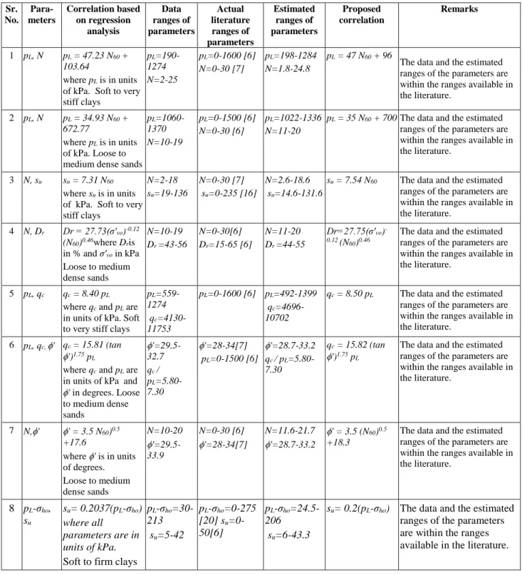
The details of the calculations of the above procedure have been presented in Table 1.

On the basis of plausibility analysis, the aforementioned mathematical correlations have been modified and the modified mathematical correlations along with their comparison with previous relevant correlative work are presented in Table 2.

Table 1: Plausibility analysis of mathematical correlations Sr. No. Para-meters Correlation based on regression analysis Data ranges of parameters Actual literature ranges of parameters Estimated ranges of parameters Proposed correlation Remarks

1 pL, N pL = 47.23 N60 + 103.64

where pL is in units of kPa. Soft to very stiff clays pL=190-1274 N=2-25 pL=0-1600 [6] N=0-30 [7] pL=198-1284 N=1.8-24.8

pL = 47 N60 + 96

The data and the estimated ranges of the parameters are within the ranges available in the literature.

2 pL, N pL = 34.93 N60 + 672.77

where pL is in units of kPa. Loose to medium dense sands

pL=1060-1370 N=10-19 pL=0-1500 [6] N=0-30 [6] pL=1022-1336 N=11-20

pL = 35 N60 + 700 The data and the estimated ranges of the parameters are within the ranges available in the literature.

3 N, su su = 7.31 N60

where su is in units of kPa. Soft to very stiff clays N=2-18 su=19-136 N=0-30 [7] su=0-235 [16] N=2.6-18.6 su=14.6-131.6

su = 7.54 N60 The data and the estimated ranges of the parameters are within the ranges available in the literature.

4 N, Dr Dr = 27.73(σ'vo)-0.12 (N60)0.46_where_Dr_is

in % and σ'vo in kPa Loose to medium dense sands N=10-19 Dr =43-56 N=0-30[6] Dr=15-65 [6] N=11-20 Dr =44-55 Dr=27.75(σ'vo) -0.12 _(N60)0.46

5 pL, qc qc = 8.40 pL

where qc and pL are in units of kPa. Soft to very stiff clays

pL=559-1274 qc=4130-11753

pL=0-1600 [6] pL=492-1399 qc=4696-10702

qc = 8.50 pL The data and the estimated ranges of the parameters are within the ranges available in the literature.

6 pL, qc, ' qc = 15.81 (tan ')1.75_pL

where qc and pL are in units of kPa and ' in degrees. Loose to medium dense sands  '=29.5-32.7 qc / pL=5.80-7.30 '=28-34[7] pL=0-1500 [6] '=28.7-33.2 qc / pL=5.80-7.30

qc = 15.82 (tan ')1.75_pL

7 N,' ' = 3.5 N60)0.5 +17.6

where ' is in units of degrees. Loose to medium dense sands N=10-20  '=29.5-33.9 N=0-30 [6] '=28-34[7] N=11.6-21.7 '=28.7-33.2

' = 3.5 (N60)0.5 +18.3

8 pL-σho,

su

su= 0.2037(pL-σho)

where all

parameters are in units of kPa. Soft to firm clays

pL-σho

=30-213 su=5-42

pL-σho=0-275

[20] su

=0-50[6]

pL-σho

=24.5-206 su=6-43.3

su= 0.2(pL-σho) The data and the estimated

ranges of the parameters are within the ranges available in the literature.

(12)

7) Conclusions

The following conclusions can be drawn from the comparison of mathematical correlations with the previous relevant correlations:

 The proposed correlations compare well with the available relevant previous literature.

 Although the proposed correlations are site specific, yet they can be used to estimate the soil parameters for the respective soil type.

 Extensive SPT data available in Pakistan can be used to anticipate design parameters of interest using the proposed correlations.

 The newly developed APMT can be employed to characterize alluvial soil deposits using both full-displacement and pre-bored techniques. However, more testing is required to build more confidence in the newly developed probe.

6. References

[1] Withers, N.J., Schaap, L.H.J. and Dalton, C.P. (1986), “The Development of a Full Displacement Pressuremeter,” The Pressuremeter and its Marine Applications: Second International Symposium. ASTM STP 950, pp 38-56.

[2] Houlsby, G.T. and Withers, N.J. (1988), “Analysis of the Cone Pressuremeter Test in Clay,” Geotechnique 38, No. 4, pp 575-587. 2: A summary of proposed and previous mathematical correlations

S. No.

Parameters Proposed correlation Previous correlation Reference

1 pL, N pL = 47 N60 + 96

where pL is in units of kPa.

Soft to very stiff clays pL = 29.45 N60 + 219.7 where pL is in units of kPa.

Medium to very stiff sandy silty clay

[13]

2 pL, N pL = 35 N60 + 700

where pL is in units of kPa.

Loose to medium dense sands

3 N, su su = 7.54 N60

where su is in units of kPa.

Soft to very stiff clays

su = 7.86 N60

where su is in units of kPa.

Very soft to stiff clays

[16]

4 N, Dr Dr = 27.75(σ'vo)-0.12 (N60)0.46

where Dris in % and σ'vo in kPa

Dr = 25(σ'vo)-0.12 (N60)0.46

where Dris in % and σ'vo in kPa.

Sand

[17]

5 pL, qc qc = 8.50 pL

where qc and pL are in units of kPa.

Soft to very stiff clays

qc = 3 pL

where qc and pL are in units of kPa.

Clay

[18]

6 pL, qc, ' qc = 15.82 (tan ')1.75 pL

where qc and pL are in units of kPa

and ' in degrees.

qc = 15 (tan ')1.75 pL

where qc and pL are in units of kPa

and' in degrees. Sand

[18]

7 N,' ' = 3.5 (N60)0.5 +18.3

where ' is in units of degrees. Loose to medium dense sands

' = 3.5 (N60)0.5 +20

where ' is in units of degrees. Sand

[19]

8 pL-σho, su su= 0.2(pL-σho)

where all parameters are in units of kPa.

Soft to firm clays

su= 0.1818(pL-σho)

where all parameters are in units of kPa.

Soft to firm clays

(13)

[3] Yu, H.S. Schnaid, F. and Collins, I.F. (1996), “Analysis of Cone Pressuremeter Tests in Sands,” Journal of Geotechnical Engineering, ASCE, Vol. 122, No.8, pp 623-632.

[4] Rehman, Z. (2010), “Development of Pressuremeter to Operate in Alluvial Soils of Punjab,” Ph.D. Thesis, Department of Civil Engineering, University of Engineering and Technology, Lahore, Pakistan.

[5] Tschebotarioff, G.P. (1973), “Foundations, Retaining, and Earth Structures, 2nd edition”,

McGraw-Hill, New York.

[6] Briaud, J.L. (1992), “The Pressuremeter,” Balkeema, Rotterdam.

[7] Bowles, J.E. (1996), “Foundation Analysis and Design,” 5th_ed_{. McGraw Hill Book Company,}

New York.

[8] Akbar, A. (2001), “Development of Low Cost In-situ Testing Devices,” Ph.D. Thesis, Department of Civil Engineering, University of Newcastle, Newcastle Upon Tyne, UK.

[9] Rehman, Z, Akbar, A. and Clarke, B. G. (2011), “Characterization of a Cohesive Soil Bed using Cone Pressuremeter”, Journal of the Japanese Geotechnical Society- Soils and Foundations, Vol. 51, No. 5, Oct. 2011, pp. 823-833.

[10] Akbar, A., Rehman, Z., Clarke, B. G. and Allen, P.G., (2010), “Development and applications of Akbar Pressuremeter, International Conference on Geotechnical Engineering, Pakistan Geotechnical Engineering Society, 5-6 November, 2010, Lahore-Pakistan, pp 87-93.

[11] Marsland, A. and Randolph, M.F. (1977), “Comparisons of Results from Pressuremeter Tests and Large In-situ Plate Tests in London Clay,” Geotechnique 27, No. 2, pp.217-243. [12] Houlsby, G.T. and Nutt, N.R.F. (1993),

“Development of the Cone Pressuremeter,”

Predictive Soil Mechanics, Proc. Wroth Memorial Symp., Oxford, pp. 254-271.

[13] Yagiz, S., Akyol, E. and Sen, G. (2008), “Relationship between the standard penetration test and the pressuremeter test on sandy silty clays: a case study from Denizli,” Bull Eng Geol Environ (2008) 67: pp 405–410.

[14] Terzaghi, K. and Peck, R.B., (1967), “Soil Mechanics in Engineering Practice”, John Wiley, New York, pp 729.

[15] Parcher, J.V. and Means, R.E. (1968), “Soil Mechanics and Foundations”, Charles E. Merrill, Columbus, Ohio.

[16] Tschebotarioff, G.P. (1973), “Foundations, Retaining, and Earth Structures, 2nd edition”,

McGraw-Hill, New York.

[17] Yoshida, Y., Ikemi, M. and Kokusho, T. (1988), “Empirical Formulas of SPT Blow Counts for Gravelly Soils”, Ist ISOPT, vol. 1: pp 381-387. [18] Van Wieringen, J.B.M. (1982), “Relating Cone

Resistance and Pressuremeter Test Results,”

Proc. 2nd Eur. Symp. Penetration Testing, Amsterdam, pp. 951-955.

[19] Muramachi, T. (1974), “Experimental Study on Application of Static Cone Penetrometer to Subsurface Investigation of Weak Cohesive Soils”, Proc. European Conf. On Penetration Testing, Stockholm, 2:2, pp 285-291.

[20] Amar, S., and Jéséquel, J.F. (1972), “Essais en place et en laboratoire sur sols cohérent comparaison des résultats”, Bull.de Liaison de LCPC, Paris, No. 58, pp97-108.