A Comparative Study on Additive and Mixed Models in Descriptive Time Series

http://www.sciencepublishinggroup.com/j/ajmcm doi: 10.11648/j.ajmcm.20200501.12

ISSN: 2578-8272 (Print); ISSN: 2578-8280 (Online)

A Comparative Study on Additive and Mixed Models in

Descriptive Time Series

Kelechukwu Celestine Nosike Dozie

1

, Maxwell Azubuike Ijomah

2, *

1

Department of Statistics Imo State University, Owerri, Imo State, Nigeria

2

Department of Mathematics/Statistics, University of Port Harcourt, Port Harcourt, Nigeria

Email address:

*_{Corresponding author}

To cite this article:

Kelechukwu Celestine Nosike Dozie, Maxwell Azubuike Ijomah. A Comparative Study on Additive and Mixed Models in Descriptive Time Series. American Journal of Mathematical and Computer Modelling. Vol. 5, No. 1, 2020, pp. 12-17. doi: 10.11648/j.ajmcm.20200501.12 Received: January 7, 2020; Accepted: January 27, 2020; Published: February 11, 2020

Abstract:

Time series analyses are statistical methods used to assess trends in repeated measurements taken at equally spaced time intervals and their relationships with other trends or events, taking account of the temporal structure of such data. An important aspect of descriptive time series analysis is the choice of model for time series decomposition. This paper examined the challenges in choosing between additive and mixed models in time series decomposition. Most of the existing studies have focused on how to choose between additive and multiplicative models with little or no regards on mixed model. The ultimate objective of this study is therefore, to compare the row, column and overall means and variances of the Buys-Ballot table for additive and mixed models. Table 1 shows that the column variances of Buys-Buys-Ballot table is constant for additive model but depends on slope and seasonal effects for mixed model. Results show that seasonal variances of the Buys-Ballot table is constant for additive model and a function of slope and seasonal effects for mixed model. Also, when there is no trend (b=0), the estimates of row, column and overall means are the same for the two models while the estimates of seasonal indices are not the same for both additive and mixed models.

Keywords:

Buys-Ballot Table, Time Series Decomposition, Additive Model, Mixed Model, Trend Parameter, Seasonal Indices

1. Introduction

An important goal in time series analysis is the decomposition of a series into a set of non-observable (latent) components that can be associated to different types of temporal variations [1]. The models most commonly used to describe time series data are additive, multiplicative and mixed models. For short series, the cyclical is embedded in the trend [2]. The decomposition models are

Additive model:

t t t t

X =M + +S e (1)

Multiplicative model:

t t t t

X =M × ×S e (2)

Mixed model:

t t t t

X =M × +S e (3)

where Mt is the trend-cycle component, St is the seasonal component and et is the error. For equation (1) it is assumed that the error term et is the Gaussian white noise

( )

2 1 0,

N

σ

and sum of the seasonal component over a complete period is zero

1 0

S

j j

S

=

 

=

 



∑

 (4)

For equation (2) it is equally assumed that the error term

t

e is the Gaussian white noise N

( )

0,

σ

12 and the sum of

1

S

j j

s S S

=

 

=

 



∑

 (5)

while for Equation (3), et is the Gaussian white noise

( )

2

1 0,

N

σ

and sum of seasonal component over a complete

period is

1

S

j j

s S S

=

 

=

 



∑

 (6)

An additive model is based on the assumption that the sum of the components is equal to the unadjusted data. In particular, this means that the fluctuations overlapping the trend-cycle are not dependent on the series level. They do not depend on the level of the trend [3].

According to [4], the appropriate model is additive when the seasonal standard deviations show no appreciable increase or decrease relative to any increase or decrease in the seasonal means. On the other hand, the appropriate model is multiplicative when the seasonal standard deviations show appreciable increase/decrease relative to any increase /decrease in the seasonal means. Here again, no statistical test was provided for the choice.

The multiplicative model was adopted when the magnitude of the seasonal pattern in the data depends on the magnitude of the series. In other words, the magnitude of the seasonal pattern increases as the data value increases and decreases as the data value decreases level of the trend. The higher the trend, the more intensive these variations are. The additive model was adopted when the magnitude of the seasonal pattern does not change as the series goes up and down while the additive model was adopted when the magnitude of the seasonal pattern does not change as the series goes up and down [5].

An important aspect of descriptive time series analysis is the choice of model for time series decomposition. The emphasis is to compare the row, column and overall means and variances of the Buys-Ballot table for additive and mixed model when trend-cycle component of time series is linear.

Iwueze and Akpanta [6] pointed out that an additive model is appropriate when the seasonal standard deviations show no appreciable increase or decrease relative to any increase or decrease in the seasonal means while a multiplicative model is usually appropriate when the seasonal standard deviations show appreciable increase/decrease relative to any increase or decrease in the seasonal means.

Linde [7] observed that, the differences between the Additive and Multiplicative and the models are (i) for the additive model, the seasonal variation is independent of the absolute level of the time series, but it takes approximately the same magnitude each year while in the multiplicative model, the seasonal variation takes the same relative magnitude each year. This is an indication that the seasonal variation equals a certain percentage of the level of the time series. The amplitude of the seasonal factor varies with the level of the time series; also for additive model, the seasonal

component is the same (roughly constant) in the same period over different years. Sometimes the seasonal component is a proportion of the underlying trend value. In such cases it is appropriate to use a multiplicative model.

Gupta [8] observed that, the additive model assumes that all the four components of the time series operate independently of each other so that none of these components has any effect on the remaining three. This means that trend may be, has no effect on the seasonal and cyclical components nor do seasonal swings have any impact on cyclical variations. According to him, this series are not independent of which other. The seasonal or cyclical variation may virtually be wiped off by very sharp and rising or declining trend. While multiplicative, model assumes that the four components of the time series are due to different causes but that, they are not necessarily independent and they can affect each other.

Oladugba et al [9] gave brief description of additive and multiplicative seasonality. According to them, the seasonal fluctuation exhibits constant amplitude with respect to the trend in additive case while amplitude of the seasonal fluctuation is a function of the trend in multiplicative seasonality.

Iwueze and Nwogu [10] observed that when the trend-cycle component is linear, the column variances of the Buys-Ballot table are constant for the additive model, but contain the seasonal component for the multiplicative model. Thus, choice between additive and multiplicative models reduces to test for constant variance to identify the additive model. They pointed out that any of the tests for constant variance can be used to identify a series that admits the additive model. This is an improvement over what is in existence. However, this approach can only identify the additive model (when the column variance is constant), but does not tell the analyst the alternative model when the variance is not constant. The implication of this is that when the test for constant variance says the appropriate model for a study series is not the additive model; an analyst still faces the challenge of distinguishing between mixed model and the multiplicative model.

2. Material and Methods

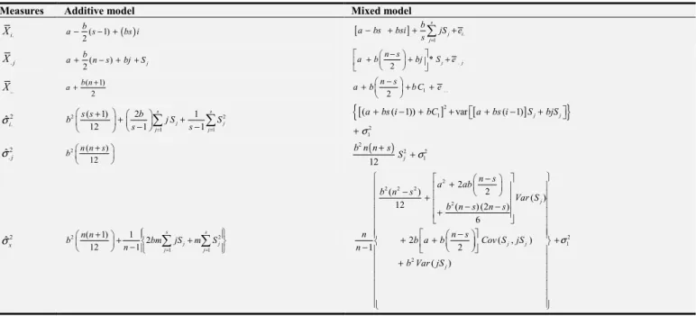
The method adopted in this study is the Buys-Ballot procedure in descriptive time series. The procedure has been developed for choice of model, among other uses, based on the row, column and overall means and variances of the Buys-Ballot table see [11-13]. For a series that has linear trend, the row, column and overall means and variances of the Buys-Ballot table for additive and mixed models are obtained by Iwueze and Nwogu [14], Nwogu el al [15] are given in Table 1.

effect in 1 1 s j j C JS = =

∑

.

2 (a) The column means mimic the shape of the trending parameters and contain seasonal indices for additive model. (b) For mixed model, the column means mimic the shape of the trending curves of the original series and contain the

seasonal indices. 3. The row and overall variances contain both trending parameters and seasonal indices for additive and mixed models. 4. The column variances of the Buys-Ballot table is constant for additive model, but a function of slope and seasonal indices for the mixed model.

Table 1. Summary of row, column and overall means and variances of Buys-Ballot for additive and mixed models.

Measures Additive model Mixed model

.

i

X ( 1) ( )

2

b

a− s− + bs i [ ] .

1

s j i j

b a bs bsi jS e

s =

− + + ∑ +

.j

X ( )

2 j

b

a+ n−s +bj+S * .

2 j j

n s

a b bj S e

 ₊  − ₊  ₊         ..

X ( 1)

2

b n

a+ + 1 . .

2

n s

a+b − +b C +e

 

2 .

ˆ_i

σ 2 2

1 1

( 1) 2 1

12 1 1

s s

j j

j j

s s b

b j S S

s = s =

 +    + +     − −     ∑ ∑ [ ] [ ]

{

2

}

1 2

1

(a bs i( 1)) bC var a bs i( 1)Sj bjSj

σ   + − + +  + − +  + 2 . ˆj

σ 2 ( )

12

n n s

b + 

  ( ) 2 2 2 1 12 j

b n n s S σ

+ +

2

ˆx

σ 2 2

1 1

( 1) 1

2 12 1 s s j j j j n n

b bm jS m S

n = =

  +     +  +    ₋    ∑ ∑  2 2 2 2

2 2 1 2 2 2 ( ) ( )

12 ( ) (2 )

6

2 ( , )

1 2 ( ) j j j j n s a ab b n s

Var S b n s n s

n n s

b a b Cov S jS n

b Var jS

σ   ₊  −     ₋  _ _    ₊     _{− −}   +          _{ − }      + + +      −       ₊             

Source: Iwueze and Nwogu (2014), Nwogu el al (2019).

These properties of row, column and overall averages and variances of the Buys-Ballot table are what could be used for estimation and assessment of trend parameters, estimation and assessment of seasonal indices and choice of the appropriate for time series decomposition.

Estimation of Trend Parameters

Row means and overall means are used to estimate parameters of the trend line. We assume that the length of periodic interval is s

For additive model, using the expression in table 1, we obtain

(

1

) ( )

2 i

b

X = −a s− + bs i (7)

i α β

≡ + (8)

where

(

1 ,

)

2

b

a s bs

α = − − β =

(

)

ˆ 1

2

b a α s

∴ = + − (9)

ˆ

b s

β

= (10)

This reduces to

i i

X = +a e (11)

when there is no trend. That is when b=0 (Table 1)

For mixed model, we obtain using the expression in Table 1

(

1

) ( )

i

X = −a b s−c + bs i ₍₁₂₎

i α β

≡ + (13)

Hence,

(

1

)

ˆ ˆ

a α b s c

∴ = + − (14)

ˆ

b s

β

= (15)

when b=0, that is when there is no trend

.

i

X = +a ei (16)

Estimates of S_j,j=1, 2,..., 5

(

)

.

2

j j j

b

X = +a n− + +s b S (17)

j Sj

α β

 

≡_ + _+ (18)

where

(

)

2

b a n s

α = − −

b

β = (19)

(

)

ˆ

2

j j j

b

S X a n s b 

∴ = − + − + 

  (20)

when there is no trend. That is when (b=0), it is clear from Table 1 that

.

ˆ

j j j

S =X − −a e ₍₂₁₎

For mixed model, we obtain using the expression in Table 1

.

2

j j j

n s X =a b−  − +bS

 

  (22)

j Sj

α β

 

≡ +  (23)

where

2

n s a b

α= +  − 

  (24)

b

β = (25)

.

ˆ

2

j j

j X S

n s

a b b

∴ =

−

 

+  +

 

(26)

When there is no trend (b=0) we obtain from (Table 1)

.

.

ˆ j

j

j X S

a e

=

+ (27)

Table 2. Estimates of Parameters for linear trending curve and seasonal indices.

Parameter Additive model Mixed model

a ˆ( 1)

2

b s

α + − α+b sˆ(−c1)

b

s

β

s

β

j

S . ( )

2

j j

b X −a+ n− +s b

 

.

2

j

j

X n s a b+_ − _+b

Note α and β are estimates obtained from the regression equations of row means on row number.

From table 2, we observed that the estimates of the trend parameters and seasonal indices are not the same for both additive and mixed.

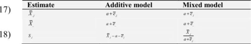
Table 3. Estimates of trend parameters and seasonal indices when there is no trend i.e. (b=0).

Estimate Additive model Mixed model

i

X a+ei a e+i

Estimate Additive model Mixed model

.j

X a+e.j a+e.j

..

X a+e.. a+e..

j

S Xj− −a ej

.

. j

j

X a e+

It is clear from Table 3 that when there is no trend i.e. (b=0), the estimates of row, column and overall means are the same for the two models while the estimates of seasonal indices are not the same for both additive and mixed models.

3. Real Life Example

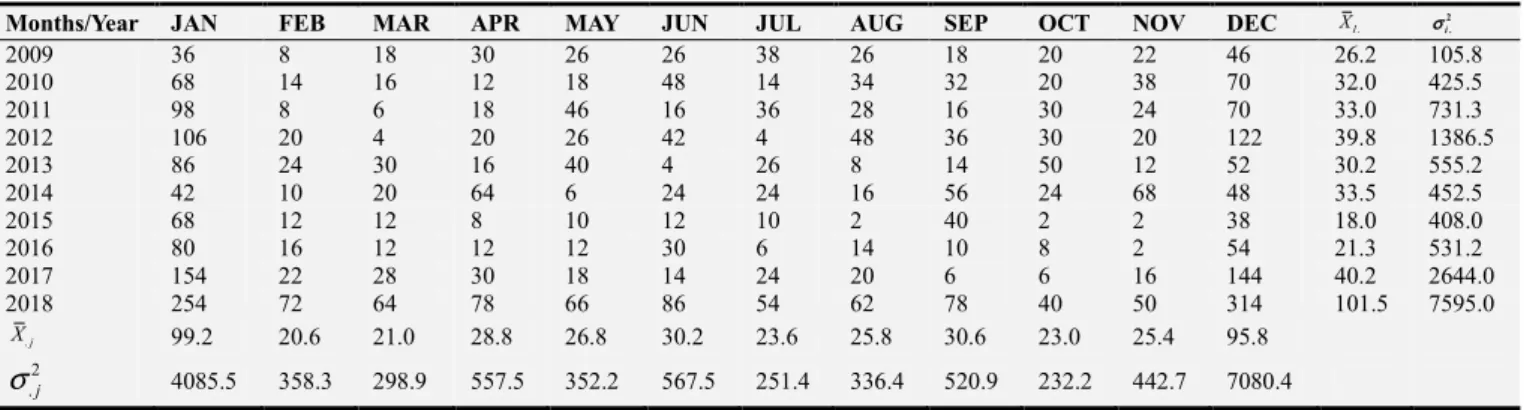
The real life example is based on monthly data on number of registered road traffic accidents in Owerri, Imo State, Nigeria for the period of 2009 to 2018 shown in Table A1. The data of 120 observations has been arranged in a Buys-Ballot table as monthly data (s = 12) and for 10 years (m = 10). The actual and transformed series are given in figures 3.1 and 3.2. The expressing of a linear trend and seasonal indices for an additive model is given as

Figure 1. Time plot of the actual series on the number of road accidents between (2009-2018).

Hence, X.j =3.0291 0.0276+ i Using (9), (10) and (20) we have

0.0276 ˆ

12

b=

0.0023

=

12 1 ˆ 3.0291 0.0023

2

a= + _ − _

 

ˆ 3.0418

a=

(

)

.

0.0023

ˆ _{3.0418 120 12 0.0023}

2

j j

S =X −_ + − + j_

 

.

ˆ _{3.166 0.0023}

j j

S =X − − j

The expression of linear trend and seasonal indices for the mixed model is given a

Hence, X_j =3.214 0.0052− j

ˆ _0.0052

b= −

(

)

120 12

ˆ 3.214 0.0052 2

a= − − _ − _

 

ˆ 3.4948

a=

.

ˆ

3.214 0.0052 j j

X S

j

= −

Figure 2. Time plot of the transformed series on the number of road accidents between (2009-2018).

Table 4. Estimates of Parameters of Trend and Seasonal Indices.

Parameter Additive model values Mixed model values ˆ

a 3.0418 3.4948

ˆ

b 0.0023 -0.0052

1

ˆ

S 1.2737 1.3823

2

ˆ

S -0.3806 0.8683

3

ˆ

S -0.4029 0.8622

4

ˆ

S -0.0722 0.9659

5

ˆ

S -0.1195 0.9521

Parameter Additive model values Mixed model values

6

ˆ

S -0.00252 0.9709

7

ˆ

S -0.2881 0.9012

8

ˆ

S -0.2554 0.9122

9

ˆ

S -0.0347 0.9818

10

ˆ

S -0.375 0.8766

11

ˆ

S -0.4233 0.8624

12

ˆ

S 1.1364 1.3492

1

ˆ s

j j

S

=

∑ 0.0000 12.0000

Note (1) Additive model satisfies

1 0

s

j j

S

=

 

=

 



∑

 as in (4)

(2) Mixed model satisfies

1

s

j j

S s

=

 

=

 



∑

 as in (6)

4. Concluding Remark

This paper has discussed the Buys-Ballot procedure for comparing the row, column and overall means and variances of the Buys-Ballot table for additive and mixed models in time series decomposition when trend-cycle component is linear. Estimates of trend parameters and seasonal indices are discussed. Results show that seasonal variances of the Buys-Ballot table is constant for additive model and a function of slope and seasonal effects for mixed model. Also, when there is no trend

(

b=0

)

, the estimates of row, column and overall means are the same for the two models while the estimates of seasonal indices are not the same for both additive and mixed models.

Appendix

Table A1. Buys-Ballot table for the data on the number of road accidents (2009-2018).

Months/Year JAN FEB MAR APR MAY JUN JUL AUG SEP OCT NOV DEC XI.

2 .

i

σ

2009 36 8 18 30 26 26 38 26 18 20 22 46 26.2 105.8

2010 68 14 16 12 18 48 14 34 32 20 38 70 32.0 425.5

2011 98 8 6 18 46 16 36 28 16 30 24 70 33.0 731.3

2012 106 20 4 20 26 42 4 48 36 30 20 122 39.8 1386.5

2013 86 24 30 16 40 4 26 8 14 50 12 52 30.2 555.2

2014 42 10 20 64 6 24 24 16 56 24 68 48 33.5 452.5

2015 68 12 12 8 10 12 10 2 40 2 2 38 18.0 408.0

2016 80 16 12 12 12 30 6 14 10 8 2 54 21.3 531.2

2017 154 22 28 30 18 14 24 20 6 6 16 144 40.2 2644.0

2018 254 72 64 78 66 86 54 62 78 40 50 314 101.5 7595.0

.j

X 99.2 20.6 21.0 28.8 26.8 30.2 23.6 25.8 30.6 23.0 25.4 95.8

2 .j

σ 4085.5 358.3 298.9 557.5 352.2 567.5 251.4 336.4 520.9 232.2 442.7 7080.4

Table A2. Buys-Ballot table for the transformed data on the number of road accidents (2009-2018).

Year Jan Feb Mar Apr May Jun Jul Aug Sep Oct Nov Dec XI.

2 .

i

σ

Year Jan Feb Mar Apr May Jun Jul Aug Sep Oct Nov Dec XI.

2 .

i

σ

2016 4.3820 2.7726 2.4849 2.4849 2.4849 3.4012 1.7918 2.6391 2.3026 2.0794 0.69312 3.9889 2.625 0.951 2017 5.0370 3.0910 3.3322 3.4012 2.8904 2.6391 3.1781 2.9957 1.7918 1.7918 2.7726 4.9698 3.158 1.014 2018 5.5373 4.2767 4.1588 4.3567 4.1897 4.4544 3.9889 4.12713 4.3567 3.6889 3.9120 5.7494 4.400 0.384

.j

X _{4.442 2.790 2.770 3.103 3.058 3.118 2.894 2.929 3.152 2.814 2.768 4.330 3.283 0.394} 2

.j

σ 0.329 0.429 0.638 0.538 0.546 0.732 0.714 0.976 0.648 0.994 1.465 0.429 3.205 0.665

Source: Federal Road Safety Corps Owerri, Imo State (2009-2018).

References

[1] Dagum E. B. (2010). Time Series Modeling and Decomposition. Statistica, anno LXX, n. 4. 434-457.

[2] Chatfield, C. (2004). The analysis of time Series: An introduction. Chapman and Hall,/CRC Press, Boca Raton. [3] Arz, S. (2006). A New Mixed Multiplicative-Additive Model

for Seasonal Adjustment. Conference on seasonality, seasonal adjustment and their implications for short-term analysis and forecasting. Luxembourg, 10-12 May.

[4] Iwueze S. I., Nwogu. E. C., Ohakwe, J., and Ajaraogu J. C. (2011). Uses of the Buys-Ballot Table in Time Series Analysis. Applied Mathematics, 2, 633-645.

[5] Enegesele D. Iwueze I. S. & Ijomah M. A. (2017). Parametric and Non Parametric Approach to Choice of Model in Descriptive Time Series International Journal of Applied Science and Mathematical Theory, 3 (4), 15-22.

[6] Iwueze, I. S. and Akpanta, A. C. (2009). “On Applying the Bartlett Transformation Method to Time Series Data”. Journal of Mathematical Sciences, Vol. 20, No. 3, pp. 227-243. [7] Linde, P. (2005). Seasonal Adjustment, Statistics Denmark.

www.dst.dk/median/konrover/13-forecasting-org/seasonal/001pdf.

[8] Gupta, S. C. (2013). Fundamentals of Statistics, Himalaya Publishing House PVT, LTD. Mumbai-400004.

[9] Oladugba, A. V., Ukaegbu, E. C., Udom, A. U., Madukaife, M. S., Ugah, T. E. & Sanni, S. S., (2014). Principles of Applied Statistic, University of Nigeria Press Limited. [10] Iwueze, I. S. & Nwogu E. C. (2004). Buys-Ballot estimates for

time series decomposition, Global Journal of Mathematics, 3 (2), 83-98.

[11] C. H. D. Buys-Ballot, “Leo Claemert Periodiques de Temperature,” Kemint et Fills, Utrecht, 1847.

[12] Iwueze S. I., Nwogu. E. C., and Ajaraogu J. C. (2015). Best Linear Unbiased Estimate using Buys-Ballot Procedure when Trend-Cycle Component is Linear. CBN Journal of Applied Statistics. 2 (1). 15–29.

[13] Okororie C. 1, Egwim K. C., Eke C. N., and Onuoha D. O., (2013). Buys-Ballot Modeling of Nigerian Domestic Crude Oil Production. West African Journal of Industrial and Academic Research 8 (1), 160-171.

[14] Iwueze, I. S. & Nwogu, E. C. (2014). Framework for choice of models and detection of seasonal effect in time series. Far East Journal of Theoretical Statistics 48 (1), 45-66.