Thorsten Joachims [email protected] Cornell University, Dept. of Computer Science, 4153 Upson Hall, Ithaca, NY 14853 USA
Abstract
This paper presents a Support Vector Method for optimizing multivariate non-linear performance measures like the F1 -score. Taking a multivariate prediction ap-proach, we give an algorithm with which such multivariate SVMs can be trained in poly-nomial time for large classes of potentially non-linear performance measures, in partic-ular ROCArea and all measures that can be computed from the contingency table. The conventional classification SVM arises as a special case of our method.
1. Introduction
Depending on the application, measuring the success of a learning algorithm requires application specific performance measures. In text classification, for ex-ample,F1-Score and Precision/Recall Breakeven Point (PRBEP) are used to evaluate classifier performance while error rate is not suitable due to a large imbal-ance between positive and negative examples. How-ever, most learning methods optimize error rate, not the application specific performance measure, which is likely to produce suboptimal results. How can we learn rules that optimize measures other than error rate? Current approaches that address this problem fall into three categories. Approaches of the first type aim to produce accurate estimates of the probabilities of class membership of each example (e.g. (Platt, 2000; Langford & Zadrozny, 2005)). While based on these probabilities many performance measures can be (ap-proximately) optimized (Lewis, 1995), estimating the probabilities accurately is a difficult problem and ar-guably harder than the original problem of optimiz-ing the particular performance measure. A second class of approaches circumvents this problem by op-Appearing inProceedings of the 22ndInternational Confer-ence on Machine Learning, Bonn, Germany, 2005. Copy-right 2005 by the author(s)/owner(s).
timizing many different variants of convenient and tractable performance measures, aiming to find one that performs well for the application specific per-formance measure after post-processing the resulting model (e.g. (Lewis, 2001; Yang, 2001; Abe et al., 2004; Caruana & Niculescu-Mizil, 2004)). However, in par-ticular for non-linear performance measures like F1 -score or PRBEP, the relationship to tractable mea-sures is at best approximate and requires extensive search via cross-validation. The final category of ap-proaches aims to directly optimize the application spe-cific performance measure. Such methods exist for some linear measures. In particular, most learning al-gorithms can be extended to incorporate unbalanced misclassification costs via linear loss functions (e.g. (Morik et al., 1999; Lin et al., 2002) in the context of SVMs). Also, methods for optimizing ROCArea have been proposed in the area of decision trees (Ferri et al., 2002), neural networks (Yan et al., 2003; Herschtal & Raskutti, 2004), boosting (Cortes & Mohri, 2003; Fre-und et al., 1998), and SVMs (Herbrich et al., 2000; Rakotomamonjy, 2004). However, for non-linear per-formance measures like F1-score, the few previous at-tempts towards their direct optimization noted their computational difficulty (Musicant et al., 2003). In this paper, we present a Support Vector Method that can directly optimize a large class of performance measures like F1-score, Precision/Recall Breakeven Point (PRBEP), Precision at k (Prec@k), and ROC-Area. One difficulty common to most application spe-cific performance measures is their non-linear and mul-tivariate nature. This results in decision theoretic risks that no longer decompose into expectations over indi-vidual examples. To accommodate this problem, we propose an approach that is fundamentally different from most conventional learning algorithms: instead of learning a univariate rule that predicts the label of a single example, we formulate the learning prob-lem as a multivariate prediction of all examples in the dataset. Based on the sparse approximation algorithm for structural SVMs (Tsochantaridis et al., 2004), we propose a method with which the training problem can be solved in polynomial time. We show that the
method applies to any performance measure that can be computed from the contingency table, as well as to the optimization of ROCArea. The new method can be thought of as a direct generalization of classification SVMs, and we show that the conventional classifica-tion SVM arises as a special case when using error rate as the performance measure. We present experiments that compare our algorithm to a conventional classifi-cation SVMs with linear cost model and observe good performance without difficult to control heuristics.
2. Multivariate Performance Measures
In this section we first review the typical assumptions (often implicitly) made by most existing learning al-gorithms (Vapnik, 1998). This gives insight into why they are not suitable for directly optimizing non-linear performance measures like theF1-Score.Most learning algorithms assume that the training dataS = ((x1, y1), ...,(xn, yn)) as well as the test data
S0 is independently identically distributed (i.i.d.) ac-cording to a learning task Pr(X, Y). The goal is to find a rule h ∈ H from the hypothesis space H that optimizes the expected prediction performance on new samplesS0 of sizen0.
R∆(h) = Z
∆ ((h(x01), ..., h(x0n0)),(y10, ..., y0n0))dPr(S0)
If the loss function ∆ over samples decomposes linearly into a sum of a loss functionδover individual examples ∆((h(x01), ..., h(x0n0)),(y01, ..., y0n0)) =
1
n0 n0
X
i=1
δ(h(x0i), yi0) (1) and since the examples are i.i.d., this expression can be simplified to
R∆(h) =Rδ(h) = Z
δ(h(x0), y0)dPr(x0, y0) Discriminative learning algorithms approximate this expected risk Rδ(h) using the empirical risk on the training dataS.
ˆ
RδS(h) = 1
n
n X
i=1
δ(h(xi), yi) (2) ˆ
Rδ
S(h) is an estimate ofRδ(h) for each h∈ H. Select-ing a rule with low empirical risk ˆRδS(h) (e.g. training error) in this decomposed form is the strategy followed by virtually all discriminative learning algorithms. However, many performance measures (e.g. F1, PRBEP) do not decompose linearly like in Eq. (1). They are a non-linear combination of the individ-ual classifications. An example is the F1 score ∆F
1((h(x1), ..., h(xn)),(y1, ..., yn)) =
2P rec Rec P rec+Rec, where
P rec and Rec are the precision and the recall of h
on the sample (x1, y1), ...,(xn, yn). There is no known example-based loss functionδwhich can be used to de-compose ∆. Therefore, learning algorithms restricted to optimizing an empirical risk of the kind in Eq. (2) are of questionable validity. What we need instead are learning algorithms that directly optimize an empirical risk that is based on the sample loss ∆.
ˆ
R∆S(h) = ∆ ((h(x1), ..., h(xn)),(y1, ..., yn))
Clearly, at least if the size n of the training set and the sizen0 of the test set are equal, ˆR∆S(h) is again an estimate ofR∆(h) for eachh∈ H. Note that ˆR∆S(h) does not necessarily have higher variance than a de-composed empirical risk ˆRδ
S(h) just because it does not “average” over multiple examples. The key factor is the variance of ∆ with respect to samples S drawn from Pr(X, Y). This variance can be low.
To design learning algorithms that do discriminative training with respect to ˆR∆
S(h), we need algorithms that find an h ∈ H that minimizes ˆR∆S(h) over the training sampleS. Since ∆ is some non-linear function ofS, this can be a challenging computational problem. We will now present a general approach to this prob-lem based on Support Vector Machines.
3. SVM Approach to Optimizing
Non-Linear Performance Measures
Support Vector Machines (SVMs) were developed by Vapnik et al. (Boser et al., 1992; Cortes & Vapnik, 1995; Vapnik, 1998) as a method for learning linear and, through the use of Kernels, non-linear rules. For the case of binary classification with unbiased hyper-planes1, SVMs learn a classifierh(x) =signwTx
by solving the following optimization problem. Optimization Problem 1. (Unbiased SVMorg)
min w,ξ≥0
1
2w·w+C n X
i=1
ξi (3)
s.t.: ∀n
i=1:yi[w·xi]≥1−ξi (4) Theξiare called slack variables. If a training example lies on the “wrong” side of the hyperplane, the corre-spondingξi is greater than 1. ThereforeP
n
i=1ξi is an upper bound on the number of training errors. This means that the SVM finds a hyperplane classifier that 1Unbiased hyperplanes assume a threshold of 0 in the classification rule. This is not a substantial restriction, since a bias can be introduced by adding an artificial fea-ture to each example.
optimizes an approximation of the training error reg-ularized by the L2 norm of the weight vector. The factorC in (3) controls the amount of regularization. To differentiate between different types of SVMs, we will denote this version as SVMorg.
In the following, we will use the same principles used in SVMorg to derive a class of SVM algorithms that optimize a broad range of non-linear performance mea-sures. The key idea is to treat the learning problem as a multivariate prediction problem. Instead of defining our hypotheses h as a function from a single feature vectorxto a single label y∈ {−1,+1},
h:X −→ Y
we will consider hypotheses ¯hthat map a tuple ¯x∈X¯ of nfeature vectors ¯x = (x1, ...,xn) to a tuple ¯y ∈Y¯ ofnlabels ¯y= (y1, ..., yn)
¯
h: ¯X −→Y¯,
where ¯X = X ×...×X and ¯Y ⊆ {−1,+1}n is the set of all admissible label vectors2. To implement this multivariate mapping, we will use linear discriminant functions of the following form.
¯
hw(¯x) = argmax ¯ y0∈Y¯
wTΨ(¯x,y¯0) (5) Intuitively, the prediction rule ¯hw(¯x) returns the tu-ple of labels ¯y0 = (y01, ..., yn0) which scores highest according to a linear function. w is a parameter vector and Ψ is a function that returns a feature vector describing the match between (x1, ...,xn) and (y10, ..., yn0). Whether this argmax can be computed ef-ficiently hinges on the structure of Ψ. For the purposes of this paper, we can restrict Ψ to be of the following simple form:
Ψ(¯x,y¯0) = n X
i=1
yi0xi
For this Ψ(¯x,y¯) and ¯Y = {−1,+1}n, the argmax is achieved when y0i is assigned to h(xi). So, in terms of the resulting classification rule, this is equivalent to SVMorg. But did we gain anything from the reformu-lation of the prediction rule?
Thinking about the prediction problem in term of a multivariate rule ¯h instead of a univariate rule h al-lows us to formulate the SVM optimization problem in a way that enables inclusion of a sample-based loss function ∆ instead of the example-based loss function in SVMorg. Following (Tsochantaridis et al., 2004), we formulate the following alternative optimization prob-lem for non-negative ∆.
2Note that ¯Y can be a strict subset for some measures, e.g. for Prec@kit is restricted to label vectors withk
pos-itive predictions.
Optimization Problem 2.(Multivar. SVM∆ multi) min
w,ξ≥0 1 2kwk
2+C ξ
s.t. ∀y¯0∈Y \¯ y¯: wT[Ψ(¯x,y¯)−Ψ(¯x,y¯0)]≥∆(¯y0,y¯)−ξ
Like for the SVMorg, this optimization problem is a convex quadratic program. In contrast to the SVMorg, however, there is one constraint for each possible ¯y∈
¯
Y. Due to the exponential size of ¯Y, this may seem like an intractably large problem. However, by adapting the sparse approximation algorithm of (Tsochantaridis et al., 2004) implemented inSVMstruct3, we will show that this problem can be solved in polynomial time for many types of multivariate loss functions ∆. Unlike in the SVMorg optimization problem there is only one slack variable ξ in this training problem. Similar to P
ξi in SVMorg, the value of this slack variable is an upper bound on the training loss.
Theorem 1. At the solution w∗, ξ∗ of the SVM∆
multi optimization problem on the training
datax¯ with labelsy¯, the value ofξ∗ is an upper bound on the training loss ∆(¯hw∗(¯x),y¯).
Proof. Let ¯y0 = ¯hw∗(¯x) be the prediction of the
learned multivariate hypothesis on the training data itself. Following from the definition of ¯h, this is the la-beling ¯y0 that minimizes w∗T[Ψ(¯x,y¯)−Ψ(¯x,y¯0)], and this quantity will be less than zero unless ¯y0 = ¯y. Therefore ξ ≥ ∆(¯y0,y¯)−wT[Ψ(¯x,y¯)−Ψ(¯x,y¯0)] ≥ ∆(¯y0,y¯).
This shows that the multivariate SVM∆multi is similar to the original SVMorg in the sense that it optimizes a convex upper bound on the training loss regularized by the norm of the weight vector. We will later show that, in fact, both formulations are identical if ∆ is the number of training errors.
It is straightforward to extend the multivariate SVM∆
multito non-linear classification rules via the dual representation of ¯h. Similar to the univariate SVMorg, the Wolfe dual of Optimization Problem 2 can be ex-pressed in terms of inner products between feature vec-tors, allowing the use of kernels. We omit this exten-sion for brevity.
4. Efficient Algorithm
How can the optimization problem of the multivariate SVM∆multi be solved despite the huge number of con-straints? This problem is a special case of the mul-tivariate prediction formulations in (Tsochantaridis et al., 2004) as well as in (Taskar et al., 2003). The
Algorithm 1 Algorithm for solving quadratic pro-gram of multivariate SVM∆multi.
1: Input: ¯x= (x1, . . . ,xn) ¯y= (y1, . . . , yn),C,, ¯Y 2: C ← ∅
3: repeat
4: y¯0←argmaxy¯0∈Y¯∆(¯y0,y¯) +wTΨ(¯x,y¯0) 5: ξ←maxy¯0∈C{max{0,∆(¯y0,y¯)−wT[Ψ(¯x,y¯)−Ψ(¯x,y¯0)]}}
6: if∆(¯y0,y¯)−wT[Ψ(¯x,y¯)−Ψ(¯x,y¯0)]> ξ+then 7: C ← C ∪ {y¯0}
8: w←optimize SVM∆
multi objective overC 9: end if
10: untilC has not changed during iteration 11: return(w)
algorithm proposed in (Taskar et al., 2003) for solving these types of large quadratic programs is not applica-ble to non-linear loss functions ∆, since it assumes that the loss decomposes linearly. The sparse approxima-tion algorithm of (Tsochantaridis et al., 2004) does not have this restriction, and we will show in the following how it can be used to solve Optimization Problem 2 in polynomial time for a large class of loss functions ∆. Algorithm 1 is the sparse approximation algorithm adapted to the multivariate SVM∆
multi. The algorithm iteratively constructs a sufficient subset of the set of constraints in Optimization Problem 2. The algorithm starts with an empty set of constraintsCand adds the currently most violated constraint in each iteration, i.e. the constraint corresponding to the label ¯y0 that maximizes ∆(¯y0,y¯) +wTΨ(¯x,y¯0). The next approxi-mation to the solution of Optimization Problem 2 is then computed on the new set of constraints. The algorithm stops when no constraint of Optimization Problem 2 is violated by more than. It is easy to see that the solutionw∗returned by Algorithm 1 fulfills all constraints up to precision, and that the norm ofw∗ is no bigger than the norm of the exact solution of Op-timization Problem 2. Furthermore, Tsochantaridis et al. (2004) show that the algorithm terminates after a polynomial number of iterations. We restate the the-orem adapted to the SVM∆
multi optimization problem. Theorem 2. For any >0and a training samplex¯ = (x1, . . . ,xn)and y¯= (y1, . . . , yn) withR= maxi||xi||
andL= maxy¯0∈Y¯∆(¯y0,y¯), Algorithm 1 terminates
af-ter incrementally adding at most
max 2L
,
8Cn2R2L 2
(6)
constraints to the working set C.
The bound is rather lose. In our experiments we ob-serve that the algorithm often converges after a few
hundred iterations even for large problems. If the search for the most violated constraint
argmax ¯ y0∈Y¯
∆(¯y0,y¯) +wTΨ(¯x,y¯0) (7) can be performed in polynomial time, the overall algo-rithm has polynomial time complexity. We will show in the following that solving the argmax efficiently is indeed possible for a large class of multivariate loss functions ∆. We will first consider multivariate loss functions that can be computed from the contingency table, and then consider the case of ROC Area. 4.1. Loss Functions Based on Contingency
Table
An exhaustive search over all ¯y0 ∈ Y¯ is not feasible. However, the computation of the argmax in Eq. (7) can be stratified over all different contingency tables,
y=1 y=-1
h(x)=1 a b
h(x)=-1 c d
so that each subproblem can be computed efficiently. Algorithm 2 is based on the observation that there are only orderO(n2) different contingency tables for a binary classification problem withnexamples. There-fore, any loss function ∆(a, b, c, d) that can be com-puted from the contingency table can take at most
O(n2) different values.
Lemma 1. Algorithm 2 computes the solution of
argmax ¯ y0∈Y¯
∆(a, b, c, d) +wTΨ(¯x,y¯0) (8)
in polynomial time for any loss function ∆(a, b, c, d)
that can be computed from the contingency table in polynomial time.
Proof. By iterating over all possible contingency ta-bles, the algorithm iterates over all possible values l
of ∆(a, b, c, d). For each contingency table (a, b, c, d) it computes the argmax over all ¯Yabcd, which is the set of ¯y that correspond to this contingency table.
¯
yabcd = argmax ¯ y0∈Y¯
abcd
wTΨ(¯x,y¯0) (9)
= argmax ¯ y0∈Y¯abcd
( n X
i=1
yi0(wTxi) )
(10)
Since the objective function is linear in ¯y0, the solution can be computed by maximizing ¯y0element wise. The maximum value for a particular contingency table is achieved when theapositive examples with the largest value of (wTx
i) are classified as positive, and the d negative examples with the lowest value of (wTx
Algorithm 2 Algorithm for computing argmax with loss functions that can be computed from the contin-gency table.
1: Input: ¯x= (x1, . . . ,xn), ¯y= (y1, . . . , yn), and ¯Y 2: (ip1, . . . , ip#pos)←sort{i:yi= 1}bywTxi 3: (in
1, . . . , in#neg)←sort{i:yi=−1}bywTxi 4: fora∈[0, . . . ,#pos]do
5: c←#pos−a
6: setyi0p
1, . . . , y 0
ipato 1 AND sety
0
ipa+1, . . . , y 0
ip#posto−1 7: ford∈[0, . . . ,#neg]do
8: b←#neg−d
9: setyi0n
1, . . . , y 0 in
bto 1 AND sety
0 in
b+1, . . . , y 0 in
#negto−1
10: v←∆(a, b, c, d) +wTPn i=1y0ixi 11: if v is the largest so farthen 12: y¯∗←(y01, ..., yn0)
13: end if
14: end for 15: end for 16: return(¯y∗)
classified as negative. The overall argmax can be com-puted by maximizing over the stratified maxima plus their constant loss.
By slightly rewriting the algorithm, it can be imple-mented to run in time O(n2). Exploiting that many loss functions are upper bounded, pruning can further improve the runtime of the algorithm. We will now give some examples of how this algorithm applies to the loss functions we will later use in experiments. Fβ-Score: The Fβ-Score is a measure typically used to evaluate binary classifiers in natural language appli-cations like text classification. It is particularly prefer-able over error rate for highly unbalanced classes. The Fβ-Score is a weighted harmonic average of Precision and Recall. It can be computed from the contingency table as
Fβ(h) =
(1 +β2)a
(1 +β2)a+b+β2c. (11) The most common choice for β is 1. For the corre-sponding loss ∆F
1(¯y
0,y¯) = 100(1−F
β), Algorithm 2 directly applies.
Precision/Recall atk In Web search engines, most users scan only the first few links that are presented. Therefore, a common way to evaluate such systems is to measure precision only on these (e.g. ten) positive predictions. Similarly, in an archival retrieval system not precision, but recall might be the most indicative measure. For example, what fraction of the total
num-ber of relevant documents did a user find after scan-ning the top 100 documents. Following this intuition, Prec@k and Rec@k measure the precision and recall of a classifier that predicts exactly k documents to be positive.
Prec@k(h) =
a
a+b Rec@k(h) = a
b+d (12)
For these measures, the space of possible prediction vectors ¯Y is restricted to those that predict exactlyk
examples to be positive. For this ¯Y, the multivariate discriminant rule ¯hw(¯x) in Eq. (5) can be computed by assigning label 1 to the k examples with highest wTxi. Similarly, a restriction to this ¯Y can easily be incorporated into Algorithm 2 by excluding all ¯y06= ¯y
from the search for whicha+b6=k.
Precision/Recall Break-Even Point The Preci-sion/Recall Break-Even Point (PRBEP) is a perfor-mance measure that is often used to evaluate text classifiers. It requires that the classifier makes a pre-diction ¯y so that precision and recall are equal, and the value of the PRBEP is defined to be equal to both. As is obvious from the definition of precision and recall, this equality is achieved for contingency tables with a+b = a+c and we restrict ¯Y appro-priately. Again, we define the corresponding loss as ∆P RBEP(¯y0,y¯) = 100(1−P RBEP) and it is straight-forward to compute ¯hw(¯x) and modify Algorithm 2 for this ¯Y.
4.2. ROC Area
ROCArea is a performance measure that cannot be computed from the contingency table, but requires predicting a ranking. However, both SVMorg and SVM∆
multi naturally predict a ranking by ordering all examples according to wTxi. From such a rank-ing, ROCArea can be computed from the number of swapped pairs
SwappedP airs=|{(i,j) : (yi> yj) and (wTxi<wTxj)}|, i.e. the number of pairs of examples that are ranked in the wrong order.
ROCArea= 1−SwappedP airs
#pos·#neg (13)
We can adapt the SVM∆
multi to optimizing ROC-Area by (implicitly) considering a classification prob-lem of all #pos·#negpairs (i, j) of a positive example (xi,1) and a negative example (xj,−1), forming a new classification problem ¯X¯ and ¯Y¯ ={−1,1}#pos·#neg as follows. Each pos/neg pair (i, j) receives the target
Algorithm 3 Algorithm for computing argmax with ROCArea-loss.
1: Input: ¯x= (x1, . . . ,xn), ¯y= (y1, . . . , yn) 2: fori∈ {i:yi= 1}dosi← −0.25 +wTxi 3: fori∈ {i:yi=−1} dosi←0.25 +wTxi 4: (r1, . . . , rn)←sort{1, . . . , n}bysi 5: sp= #pos,sn= 0
6: fori∈ {1, . . . , n}do 7: if yri >0 then
8: cri ←(#neg−2sn)
9: sp ←sp−1 10: else
11: cri ←(−#pos+ 2sp)
12: sn ←sn+ 1 13: end if
14: end for
15: return(c1, . . . , cn)
label yij = 1 and is described by the feature vector xij = xi−xj. In this representation, the discrim-inant rule ¯¯hw(¯x¯) = argmaxy¯¯0∈Y¯¯
wTΨ(¯x¯,y¯¯0) corre-sponds to labeling a pair (i, j) assign(wTx
i−wTxj), i.e. according to the ordering w.r.t wTx
i as desired. Note that the error between the prediction ¯y¯0 and the true pairwise labels ¯y¯ = (1, ...,1)T is proportional to 1−ROCArea of the original data ¯x and ¯y. We call this quantity the ROCArea-loss.
∆ROCArea(¯y¯0,y¯¯) = n X i=1 n X j=1 1 2(1−y
0
ij) =SwappedP airs
Actually representing all #pos·#neg pairs would be rather inefficient, but can be avoided using the fol-lowing representation which is linear in the number of examples n.
Ψ(¯¯x,y¯¯) = n X
i=1
cixi withci=
( P#neg
j=1 yij, if(yi= 1)
−P#pos
j=1 yji, if(yi=−1) Note that ∆ROCArea(¯y¯0,y¯¯) can now be computed as ∆ROCArea(¯y¯0,y¯¯) = 12Pni=1yi(ci−c0i). Algorithm 3 computes the argmax in this representation.
Lemma 2. Forx¯ andy¯ of sizen, Algorithm 3 com-putes the solutionc1, . . . , cn corresponding to
argmax ¯ ¯ y0∈Y¯¯
∆ROCArea(¯y¯0,y¯¯) +wTΨ(¯x¯,y¯¯0) (14)
in timeO(nlogn).
Proof. The argmax can be written as follows in the pairwise representation.
¯ ¯
y∗ = argmax ¯ ¯ y0∈Y¯
#pos X i=1 #neg X j=1 1 2(1−y
0
ij) +y0ijw T
(xi−xj)
Since the loss function decomposes linearly over the pairwise representation, we can maximize eachyij in-dividually.
yij∗ = argmax y0
ij∈{−1,+1}
1 2(1−y
0
ij) +yij0 wT(xi−xj)
= argmax
y0
ij∈{−1,+1}
yij[(wTxi− 1 4)−(w
Txj+1 4)] This means that a pair (i, j) should be labeled as
yij = 1, if the score wTxi of the positive example decremented by 14 is larger than the scorewTxj of the negative example incremented by 1
4. This is precisely how the algorithm assigns the labels and collects them in the compressed representation. The runtime of the algorithm is dominated by a single sort operation.
5. SVM
∆multi
Generalizes SVM
orgThe following theorem shows that the multivariate SVM∆
multiis a direct generalization of the conventional classification SVM. When using error rate as the loss function, the conventional SVM arises as a special case of SVM∆
multi.
Theorem 3. Using error as the loss function, in par-ticular ∆Err(¯y0,y¯) = 2 (b+c), SVMErrmulti with
regu-larization parameterCmulti computes the same
hyper-plane w as SVMorg withCorg= 2Cmulti.
Proof. We will show that both optimization problems have the same objective value and an equivalent set of constraints. In particular, for everyw the smallest feasibleξandP
iξi are related asξ= 2 P
iξi. For a given w, the ξi in SVMorg can be optimized individually, and the optimum is achieved for ξi =
max{0,1−yi(wTxi)}. For the SVMErrmulti, the optimal
ξfor a given wis
ξ= max ¯ y0∈Y¯
(
∆Err(¯y0,y¯) + n X
i=1
y0iwTxi− n X
i=1
yiwTxi )
Since the function is linear in the y0i, each yi0 can be optimized independently. Denote withδErr(yi0, yi) the univariate loss function that returns 2 if both argu-ments differ, and 0 otherwise.
ξ = n X i=1 max y0
i∈{−1,+1}
δErr(y0i, yi) +yi0w Tx
i−yiwTxi
= n X
i=1 max
0,2−2yiwTxi = 2 n X
i=1
ξi
Therefore, if Corg = 2Cmulti, the objective functions of both optimization problems are equal for any w, and consequently so are their optima w.r.t. w.
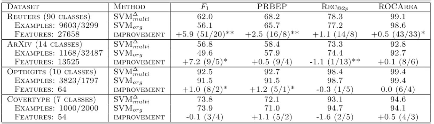
Table 1.Comparing an SVM optimized for the performance measure to one that is trained with linear cost model.
Dataset Method F1 PRBEP Rec@2p ROCArea
Reuters (90 classes) SVM∆multi 62.0 68.2 78.3 99.1
Examples: 9603/3299 SVMorg 56.1 65.7 77.2 98.6
Features: 27658 improvement +5.9 (51/20)** +2.5 (16/8)** +1.1 (14/8) +0.5 (43/33)*
ArXiv (14 classes) SVM∆multi 56.8 58.4 73.3 92.8
Examples: 1168/32487 SVMorg 49.6 57.9 74.4 92.7
Features: 13525 improvement +7.2 (9/5)* +0.5 (9/4) -1.1 (1/13)** +0.1 (8/6)
Optdigits (10 classes) SVM∆multi 92.5 92.7 98.4 99.4
Examples: 3823/1797 SVMorg 91.5 91.5 98.7 99.4
Features: 64 improvement +1.0 (8/2)* +1.2 (5/1)* -0.3 (1/5) 0.0 (6/4)
Covertype (7 classes) SVM∆multi 73.8 72.1 93.1 94.6
Examples: 1000/2000 SVMorg 73.9 71.0 94.7 94.1
Features: 54 improvement -0.1 (3/4) +1.1 (5/2) -1.6 (2/5) +0.5 (4/3)
6. Experiments
To evaluate the proposed SVM approach to optimizing non-linear performance measures, we conducted exper-iments on four different test collection. We compare
F1-score, PRBEP, Rec@k for k twice the number of positive examples (Rec@2p), and ROCArea achieved by the respective SVM∆
multi with the performance of a classification SVM that includes a cost model. The cost model is implemented by allowing different reg-ularization constants for positive and negative exam-ples (Morik et al., 1999). Using the parameter j of
SVMlight, the C parameter of positive examples is multiplied byj to increase their influence. This setup is a strong baseline to compare against. For exam-ple, David Lewis won the TREC-2001 Batch Filtering Evaluation (Lewis, 2001) using SVMlight with such cost models. Furthermore, Musicant et al. (2003) make a theoretical argument that such cost models approximately optimizeF1-score.
We compare performance on four test collections, namely the ModApte Reuters-21578 text classification benchmark4, a dataset of abstracts from the Physics E-Print ArXiv, and the OPTDIGITS and COVER-TYPE benchmarks5. Train/test split and the number of features are given in Table 1.
Initial experiments indicated that biased hyperplane (i.e. adjustable threshold) outperform unbiased hy-perplanes. We therefore add a constant feature with value 1 to each training example for the SVM∆multiand use biased hyperplanes for the regular SVM as imple-mented inSVMlight. To select the regularization para-meterCfor the SVM∆
multi, andCandjfor the classifi-cation SVM, we used holdout testing with a random 2 3 / 1
3split of the training set for each class in a collection. 4
http://www.daviddlewis.com/ 5
http://www.ics.uci.edu/∼mlearn/MLRepository.html
We search withinC ∈[2−6, ...,26] andj ∈[20, ...,27], but extended the search space if the most frequently selected parameter setting over all classes in the col-lection was on a boundary.
Our implementation of SVM∆
multi is available at http://svmlight.joachims.org.
Table 1 shows the macro-average of the performance over all classes in a collection. Each “improvement” line shows the amount by which the SVM∆
multi out-performs (or underout-performs) the regular SVM. Both the difference in performance, as well as the number of classes on which the SVM∆multi won/lost are shown. Stars indicate the level of significance according to a two-tailed Wilcoxon test applied to pairs of results over classes. One star indicates a significance level of 0.9, two stars a level of 0.95. Overall, 11 macroaverages in Table 1 show an improvement (6 significant), and only 4 cases (1 significant) show a decline in perfor-mance. Comparing the results between datasets, the improvements are largest for the two text classification tasks, while especially for COVERTYPE there is no significant difference between the two methods. With respect to different performance measures, the largest gains are observed forF1-score on the text classifica-tion tasks. PRBEP and ROCArea also show consis-tent, but smaller gains. On Rec@2p, the regular SVM appears to perform better on average.
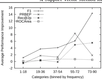
Figure 1 further analyzes how the performance differs between the individual binary tasks in the Reuters col-lection. The 90 tasks were binned into 5 sets by their ratio of positive to negative examples. Figure 1 plots the average performance improvement in each bin from the most popular classes on the left to the least popu-lar classes on the right. For most measures, especially
F1-score, improvements are larger for the less popular categories.
-2 0 2 4 6 8 10 12 14 16
1-18 19-36 37-54 55-72 73-90
Average Performance Improvement
Categories (binned by frequency) F1
PRBEP Rec@2p ROCArea
Figure 1.Improvement in prediction performance on Reuters of SVM∆
multi over SVMorg depending on the
bal-ance between positive and negative examples. Results are averaged by binning the 90 categories according to their number of examples.
7. Conclusions
This paper generalized SVMs to optimizing large classes of multivariate non-linear performance mea-sures often encountered in practical applications. We presented a training algorithm and showed that is it computationally tractable. The new approach leads to improved performance particularly for text classifi-cation problems with highly unbalanced classes. Fur-thermore, it provides a principled approach to opti-mizing such measures and avoids difficult to control heuristics.
This work was funded in part under NSF awards IIS-0412894 and IIS-0412930.
References
Abe, N., Zadrozny, B., & Langford, J. (2004). An iter-ative method for multi-class cost-sensitive learning.
Proc. KDD.
Boser, B. E., Guyon, I. M., & Vapnik, V. N. (1992). A traininig algorithm for optimal margin classifiers.
Proc. COLT.
Caruana, R., & Niculescu-Mizil, A. (2004). Data min-ing in metric space: an empirical analysis of super-vised learning performance criteria. Proc. KDD. Cortes, C., & Mohri, M. (2003). Auc optimization vs.
error rate minimization. Proc. NIPS.
Cortes, C., & Vapnik, V. N. (1995). Support–vector networks. Machine Learning, 20, 273–297.
Ferri, C., Flach, P., & Hernandez-Orallo, J. (2002). Learning decision trees using the area under the roc curve. Proc. ICML.
Freund, Y., Iyer, R., Schapire, R., & Singer, Y. (1998). An efficient boosting algorithm for combining pref-erences. Proc. ICML.
Herbrich, R., Graepel, T., & Obermayer, K. (2000). Large margin rank boundaries for ordinal regression. In et A. S. al. (Ed.),Advances in large margin clas-sifiers. MIT Press.
Herschtal, A., & Raskutti, B. (2004). Optimising area under the roc curve using gradient descent. Proc. ICML.
Langford, J., & Zadrozny, B. (2005). Estimating class membership probabilities using classifier learners.
Proc. AISTATS.
Lewis, D. (1995). Evaluating and optimizing au-tonomous text classification systems. Proc. SIGIR. Lewis, D. (2001). Applying support vector machines to the trec-2001 batch filtering and routing tasks.
Proc. TREC.
Lin, Y., Lee, Y., & Wahba, G. (2002). Support vec-tor machines for classification in nonstandard situ-ations. Machine Learning,46, 191 – 202.
Morik, K., Brockhausen, P., & Joachims, T. (1999). Combining statistical learning with a knowledge-based approach. Proc. ICML.
Musicant, D., Kumar, V., & Ozgur, A. (2003). Op-timizing f-measure with support vector machines.
Proc. FLAIRS.
Platt, J. (2000). Probabilistic outputs for support vec-tor machines and comparisons to regularized likeli-hood methods. In et A. S. al. (Ed.), Advances in large margin classifiers. MIT Press.
Rakotomamonjy, A. (2004). Svms and area under roc curve(Technical Report). PSI-INSA de Rouen. Taskar, B., Guestrin, C., & Koller, D. (2003).
Maximum-margin markov networks. Proc. NIPS. Tsochantaridis, I., Hofmann, T., Joachims, T., &
Al-tun, Y. (2004). Support vector machine learning for interdependent and structured output spaces. Proc. ICML.
Vapnik, V. (1998). Statistical learning theory. Wiley. Yan, L., Dodier, R., Mozer, M., & Wolniewicz, R.
(2003). Optimizing classifier performance via ap-proximation to the wilcoxon-mann-witney statistic.
Proc. ICML.
Yang, Y. (2001). A study of thresholding strategies for text categorization. Proc. SIGIR.