Chapter 1
PRINCIPAL COMPONENT ANALYSIS
Introduction: The Basics of Principal Component Analysis . . . 2
A Variable Reduction Procedure . . . 2
An Illustration of Variable Redundancy . . . 3
What is a Principal Component? . . . 5
How principal components are computed . . . 5
Number of components extracted . . . 7
Characteristics of principal components . . . 7
Orthogonal versus Oblique Solutions . . . 8
Principal Component Analysis is Not Factor Analysis . . . 9
Example: Analysis of the Prosocial Orientation Inventory . . . 10
Preparing a Multiple-Item Instrument . . . 11
Number of Items per Component . . . 12
Minimally Adequate Sample Size . . . 13
SAS Program and Output . . . 13
Writing the SAS Program . . . 14
The DATA step . . . 14
The PROC FACTOR statement . . . 15
Options used with PROC FACTOR . . . 15
The VAR statement . . . 17
Example of an actual program . . . 17
Results from the Output . . . 17
Steps in Conducting Principal Component Analysis . . . 21
Step 1: Initial Extraction of the Components . . . 21
Step 2: Determining the Number of “Meaningful” Components to Retain . . . 22
Step 3: Rotation to a Final Solution . . . 28
Factor patterns and factor loadings . . . 28
Rotations . . . 28
Step 4: Interpreting the Rotated Solution . . . 28
Step 5: Creating Factor Scores or Factor-Based Scores . . . 31
Computing factor scores . . . 32
Computing factor-based scores . . . 36
Recoding reversed items prior to analysis . . . 38
Step 6: Summarizing the Results in a Table . . . 40
An Example with Three Retained Components . . . 41
The Questionnaire . . . 41
Writing the Program . . . 43
Results of the Initial Analysis . . . 44
Results of the Second Analysis . . . 50
Conclusion . . . 55
Appendix: Assumptions Underlying Principal Component Analysis . . . 55
References . . . 56
Overview. This chapter provides an introduction to principal component analysis: a variable-reduction procedure similar to factor analysis. It provides guidelines regarding the necessary sample size and number of items per component. It shows how to determine the number of components to retain, interpret the rotated solution, create factor scores, and summarize the results. Fictitious data from two studies are analyzed to illustrate these procedures. The present chapter deals only with the creation of orthogonal (uncorrelated) components; oblique (correlated) solutions are covered in Chapter 2, “Exploratory Factor Analysis”.
Introduction: The Basics of Principal Component Analysis
Principal component analysis is appropriate when you have obtained measures on a number of observed variables and wish to develop a smaller number of artificial variables (called principal components) that will account for most of the variance in the observed variables. The principal components may then be used as predictor or criterion variables in subsequent analyses.
A Variable Reduction Procedure
Principal component analysis is a variable reduction procedure. It is useful when you have obtained data on a number of variables (possibly a large number of variables), and believe that there is some redundancy in those variables. In this case, redundancy means that some of the variables are correlated with one another, possibly because they are measuring the same construct. Because of this redundancy, you believe that it should be possible to reduce the observed variables into a smaller number of principal components (artificial variables) that will account for most of the variance in the observed variables.
Because it is a variable reduction procedure, principal component analysis is similar in many respects to exploratory factor analysis. In fact, the steps followed when conducting a principal component analysis are virtually identical to those followed when conducting an exploratory factor analysis. However, there are significant conceptual differences between the two
procedures, and it is important that you do not mistakenly claim that you are performing factor analysis when you are actually performing principal component analysis. The differences between these two procedures are described in greater detail in a later section titled “Principal Component Analysis is Not Factor Analysis.”
An Illustration of Variable Redundancy
A specific (but fictitious) example of research will now be presented to illustrate the concept of variable redundancy introduced earlier. Imagine that you have developed a 7-item measure of job satisfaction. The instrument is reproduced here:
Please respond to each of the following statements by placing a rating in the space to the left of the statement. In making your ratings, use any number from 1 to 7 in which 1=“strongly disagree” and 7=“strongly agree.”
_____ 1. My supervisor treats me with consideration.
_____ 2. My supervisor consults me concerning important decisions that affect my work.
_____ 3. My supervisors give me recognition when I do a good job. _____ 4. My supervisor gives me the support I need to do my job
well.
_____ 5. My pay is fair.
_____ 6. My pay is appropriate, given the amount of responsibility that comes with my job.
_____ 7. My pay is comparable to the pay earned by other employees whose jobs are similar to mine.
Perhaps you began your investigation with the intention of administering this questionnaire to 200 or so employees, and using their responses to the seven items as seven separate variables in subsequent analyses (for example, perhaps you intended to use the seven items as seven separate predictor variables in a multiple regression equation in which the criterion variable was
There are a number of problems with conducting the study in this fashion, however. One of the more important problems involves the concept of redundancy that was mentioned earlier. Take a close look at the content of the seven items in the questionnaire. Notice that items 1-4 all deal with the same topic: the employees’ satisfaction with their supervisors. In this way, items 1-4 are somewhat redundant to one another. Similarly, notice that items 5-7 also all seem to deal with the same topic: the employees’ satisfaction with their pay.
Empirical findings may further support the notion that there is redundancy in the seven items. Assume that you administer the questionnaire to 200 employees and compute all possible correlations between responses to the 7 items. The resulting fictitious correlations are reproduced in Table 1.1:
Table 1.1
Correlations among Seven Job Satisfaction Items
_______________________________________________________
Correlations
__________________________________________
Variable 1 2 3 4 5 6 7 _______________________________________________________
1 1.00
2 .75 1.00
3 .83 .82 1.00
4 .68 .92 .88 1.00
5 .03 .01 .04 .01 1.00
6 .05 .02 .05 .07 .89 1.00
7 .02 .06 .00 .03 .91 .76 1.00
__________________________________________________________________
Note : N = 200.
When correlations among several variables are computed, they are typically summarized in the form of a correlation matrix, such as the one reproduced in Table 1.1. This is an appropriate opportunity to review just how a correlation matrix is interpreted. The rows and columns of
Table 1.1 correspond to the seven variables included in the analysis: Row 1 (and column 1) represents variable 1, row 2 (and column 2) represents variable 2, and so forth. Where a given row and column intersect, you will find the correlation between the two corresponding variables. For example, where the row for variable 2 intersects with the column for variable 1, you find a correlation of .75; this means that the correlation between variables 1 and 2 is .75.
The correlations of Table 1.1 show that the seven items seem to hang together in two distinct groups. First, notice that items 1-4 show relatively strong correlations with one another. This could be because items 1-4 are measuring the same construct. In the same way, items 5-7 correlate strongly with one another (a possible indication that they all measure the same construct as well). Even more interesting, notice that items 1-4 demonstrate very weak correlations with items 5-7. This is what you would expect to see if items 1-4 and items 5-7 were measuring two different constructs.
Given this apparent redundancy, it is likely that the seven items of the questionnaire are not really measuring seven different constructs; more likely, items 1-4 are measuring a single construct that could reasonably be labelled “satisfaction with supervision,” while items 5-7 are measuring a different construct that could be labelled “satisfaction with pay.”
If responses to the seven items actually displayed the redundancy suggested by the pattern of correlations in Table 1.1, it would be advantageous to somehow reduce the number of variables in this data set, so that (in a sense) items 1-4 are collapsed into a single new variable that reflects the employees’ satisfaction with supervision, and items 5-7 are collapsed into a single new variable that reflects satisfaction with pay. You could then use these two new artificial variables (rather than the seven original variables) as predictor variables in multiple regression, or in any other type of analysis.
In essence, this is what is accomplished by principal component analysis: it allows you to reduce a set of observed variables into a smaller set of artificial variables called principal components. The resulting principal components may then be used in subsequent analyses.
What is a Principal Component?
How principal components are computed. Technically, a principal component can be defined as a linear combination of optimally-weighted observed variables. In order to
understand the meaning of this definition, it is necessary to first describe how subject scores on a principal component are computed.
In the course of performing a principal component analysis, it is possible to calculate a score for each subject on a given principal component. For example, in the preceding study, each subject would have scores on two components: one score on the satisfaction with supervision
component, and one score on the satisfaction with pay component. The subject’s actual scores on the seven questionnaire items would be optimally weighted and then summed to compute their scores on a given component.
Below is the general form for the formula to compute scores on the first component extracted (created) in a principal component analysis:
C1 = b11(X1) + b12(X2) + ... b1p(Xp)
where
C1 = the subject’s score on principal component 1 (the first component extracted) b1p = the regression coefficient (or weight) for observed variable p, as used in
creating principal component 1
Xp = the subject’s score on observed variable p.
For example, assume that component 1 in the present study was the “satisfaction with
supervision” component. You could determine each subject’s score on principal component 1 by using the following fictitious formula:
C1 = .44 (X1) + .40 (X2) + .47 (X3) + .32 (X4)
+ .02 (X5) + .01 (X6) + .03 (X7)
In the present case, the observed variables (the “X” variables) were subject responses to the seven job satisfaction questions; X1 represents question 1, X2 represents question 2, and so forth. Notice that different regression coefficients were assigned to the different questions in
computing subject scores on component 1: Questions 1– 4 were assigned relatively large regression weights that range from .32 to 44, while questions 5 –7 were assigned very small weights ranging from .01 to .03. This makes sense, because component 1 is the satisfaction with supervision component, and satisfaction with supervision was assessed by questions 1– 4. It is therefore appropriate that items 1– 4 would be given a good deal of weight in computing subject scores on this component, while items 5 –7 would be given little weight.
Obviously, a different equation, with different regression weights, would be used to compute subject scores on component 2 (the satisfaction with pay component). Below is a fictitious illustration of this formula:
C2 = .01 (X1) + .04 (X2) + .02 (X3) + .02 (X4)
+ .48 (X5) + .31 (X6) + .39 (X7)
The preceding shows that, in creating scores on the second component, much weight would be given to items 5 –7, and little would be given to items 1– 4. As a result, component 2 should
account for much of the variability in the three satisfaction with pay items; that is, it should be strongly correlated with those three items.
At this point, it is reasonable to wonder how the regression weights from the preceding equations are determined. The SAS System’s PROC FACTOR solves for these weights by using a special type of equation called an eigenequation. The weights produced by these eigenequations are optimal weights in the sense that, for a given set of data, no other set of weights could produce a set of components that are more successful in accounting for variance in the observed variables. The weights are created so as to satisfy a principle of least squares similar (but not identical) to the principle of least squares used in multiple regression. Later, this chapter will show how PROC FACTOR can be used to extract (create) principal components.
It is now possible to better understand the definition that was offered at the beginning of this section. There, a principal component was defined as a linear combination of optimally weighted observed variables. The words “linear combination” refer to the fact that scores on a component are created by adding together scores on the observed variables being analyzed. “Optimally weighted” refers to the fact that the observed variables are weighted in such a way that the resulting components account for a maximal amount of variance in the data set.
Number of components extracted . The preceding section may have created the impression that, if a principal component analysis were performed on data from the 7-item job satisfaction questionnaire, only two components would be created. However, such an impression would not be entirely correct.
In reality, the number of components extracted in a principal component analysis is equal to the number of observed variables being analyzed. This means that an analysis of your 7-item questionnaire would actually result in seven components, not two.
However, in most analyses, only the first few components account for meaningful amounts of variance, so only these first few components are retained, interpreted, and used in subsequent analyses (such as in multiple regression analyses). For example, in your analysis of the 7-item job satisfaction questionnaire, it is likely that only the first two components would account for a meaningful amount of variance; therefore only these would be retained for interpretation. You would assume that the remaining five components accounted for only trivial amounts of variance. These latter components would therefore not be retained, interpreted, or further analyzed.
Characteristics of principal components. The first component extracted in a principal
component analysis accounts for a maximal amount of total variance in the observed variables. Under typical conditions, this means that the first component will be correlated with at least some of the observed variables. It may be correlated with many.
The second component extracted will have two important characteristics. First, this component will account for a maximal amount of variance in the data set that was not accounted for by the first component. Again under typical conditions, this means that the second component will be
correlated with some of the observed variables that did not display strong correlations with component 1.
The second characteristic of the second component is that it will be uncorrelated with the first component. Literally, if you were to compute the correlation between components 1 and 2, that correlation would be zero.
The remaining components that are extracted in the analysis display the same two characteristics: each component accounts for a maximal amount of variance in the observed variables that was not accounted for by the preceding components, and is uncorrelated with all of the preceding components. A principal component analysis proceeds in this fashion, with each new component accounting for progressively smaller and smaller amounts of variance (this is why only the first few components are usually retained and interpreted). When the analysis is complete, the
resulting components will display varying degrees of correlation with the observed variables, but are completely uncorrelated with one another.
What is meant by “total variance” in the data set? To understand the meaning of “total variance” as it is used in a principal component analysis, remember that the observed variables are standardized in the course of the analysis. This means that each variable is transformed so that it has a mean of zero and a variance of one. The “total variance” in the data set is simply the sum of the variances of these observed variables. Because they have been standardized to have a variance of one, each observed variable contributes one unit of variance to the “total variance” in the data set. Because of this, the total variance in a principal component analysis will always be equal to the number of observed variables being analyzed. For example, if seven variables are being analyzed, the total variance will equal seven. The components that are extracted in the analysis will partition this variance: perhaps the first component will account for 3.2 units of total variance; perhaps the second component will account for 2.1 units. The analysis continues in this way until all of the variance in the data set has been accounted for.
Orthogonal versus Oblique Solutions
This chapter will discuss only principal component analyses that result in orthogonal solutions. An orthogonal solution is one in which the components remain uncorrelated (orthogonal means “uncorrelated”).
It is possible to perform a principal component analysis that results in correlated components. Such a solution is called an oblique solution. In some situations, oblique solutions are superior to orthogonal solutions because they produce cleaner, more easily-interpreted results.
However, oblique solutions are also somewhat more complicated to interpret, compared to orthogonal solutions. For this reason, the present chapter will focus only on the interpretation of
orthogonal solutions. To learn about oblique solutions, see Chapter 2. The concepts discussed in this chapter will provide a good foundation for the somewhat more complex concepts discussed in that chapter.
Principal Component Analysis is Not Factor Analysis
Principal component analysis is sometimes confused with factor analysis, and this is
understandable, because there are many important similarities between the two procedures: both are variable reduction methods that can be used to identify groups of observed variables that tend to hang together empirically. Both procedures can be performed with the SAS System’s
FACTOR procedure, and they sometimes even provide very similar results.
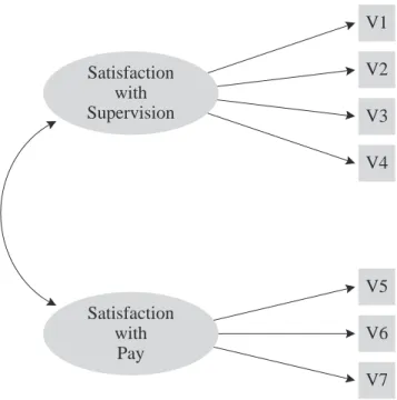
Nonetheless, there are some important conceptual differences between principal component analysis and factor analysis that should be understood at the outset. Perhaps the most important deals with the assumption of an underlying causal structure: factor analysis assumes that the covariation in the observed variables is due to the presence of one or more latent variables (factors) that exert causal influence on these observed variables. An example of such a causal structure is presented in Figure 1.1:
V1 V2 V3 V4 Satisfaction
with Supervision
Satisfaction with
Pay
V5 V6 V7
Figure 1.1: Example of the Underlying Causal Structure that is Assumed in Factor Analysis
The ovals in Figure 1.1 represent the latent (unmeasured) factors of “satisfaction with supervision” and “satisfaction with pay.” These factors are latent in the sense that they are assumed to actually exist in the employee’s belief systems, but cannot be measured directly. However, they do exert an influence on the employee’s responses to the seven items that constitute the job satisfaction questionnaire described earlier (these seven items are represented
as the squares labelled V1-V7 in the figure). It can be seen that the “supervision” factor exerts influence on items V1-V4 (the supervision questions), while the “pay” factor exerts influence on items V5-V7 (the pay items).
Researchers use factor analysis when they believe that certain latent factors exist that exert causal influence on the observed variables they are studying. Exploratory factor analysis helps the researcher identify the number and nature of these latent factors.
In contrast, principal component analysis makes no assumption about an underlying causal model. Principal component analysis is simply a variable reduction procedure that (typically) results in a relatively small number of components that account for most of the variance in a set of observed variables.
In summary, both factor analysis and principal component analysis have important roles to play in social science research, but their conceptual foundations are quite distinct.
Example: Analysis of the Prosocial Orientation Inventory
Assume that you have developed an instrument called the Prosocial Orientation Inventory (POI) that assesses the extent to which a person has engaged in helping behaviors over the preceding six-month period. The instrument contains six items, and is reproduced here.
Instructions: Below are a number of activities that people sometimes engage in. For each item, please indicate how
frequently you have engaged in this activity over the preceding six months. Make your rating by circling the appropriate number to the left of the item, and use the following response format:
7 = Very Frequently 6 = Frequently
5 = Somewhat Frequently 4 = Occasionally
3 = Seldom
2 = Almost Never 1 = Never
1 2 3 4 5 6 7 1. Went out of my way to do a favor for a coworker.
1 2 3 4 5 6 7 2. Went out of my way to do a favor for a relative.
1 2 3 4 5 6 7 3. Went out of my way to do a favor for a friend.
1 2 3 4 5 6 7 4. Gave money to a religious charity.
1 2 3 4 5 6 7 5. Gave money to a charity not associated with a religion.
1 2 3 4 5 6 7 6. Gave money to a panhandler.
When you developed the instrument, you originally intended to administer it to a sample of subjects and use their responses to the six items as six separate predictor variables in a multiple regression equation. However, you have recently learned that this would be a questionable practice (for the reasons discussed earlier), and have now decided to instead perform a principal component analysis on responses to the six items to see if a smaller number of components can successfully account for most of the variance in the data set. If this is the case, you will use the resulting components as the predictor variables in your multiple regression analyses.
At this point, it may be instructive to review the content of the six items that constitute the POI to make an informed guess as to what you are likely to learn from the principal component analysis. Imagine that, when you first constructed the instrument, you assumed that the six items were assessing six different types of prosocial behavior. However, inspection of items 1-3 shows that these three items share something in common: they all deal with the activity of “going out of one’s way to do a favor for an acquaintance.” It would not be surprising to learn that these three items will hang together empirically in the principal component analysis to be performed. In the same way, a review of items 4-6 shows that all of these items involve the activity of “giving money to the needy.” Again, it is possible that these three items will also group together in the course of the analysis.
In summary, the nature of the items suggests that it may be possible to account for the variance in the POI with just two components: An “acquaintance helping” component, and a “financial giving” component. At this point, we are only speculating, of course; only a formal analysis can tell us about the number and nature of the components measured by the POI.
(Remember that the preceding fictitious instrument is used for purposes of illustration only, and should not be regarded as an example of a good measure of prosocial orientation; among other problems, this questionnaire obviously deals with very few forms of helping behavior).
Preparing a Multiple-Item Instrument
The preceding section illustrates an important point about how not to prepare a multiple-item measure of a construct: Generally speaking, it is poor practice to throw together a questionnaire, administer it to a sample, and then perform a principal component analysis (or factor analysis) to see what the questionnaire is measuring.
Better results are much more likely when you make a priori decisions about what you want the questionnaire to measure, and then take steps to ensure that it does. For example, you would have been more likely to obtain desirable results if you:
• had begun with a thorough review of theory and research on prosocial behavior • used that review to determine how many types of prosocial behavior probably exist • wrote multiple questionnaire items to assess each type of prosocial behavior.
Using this approach, you could have made statements such as “There are three types of prosocial behavior: acquaintance helping, stranger helping, and financial giving.” You could have then prepared a number of items to assess each of these three types, administered the questionnaire to a large sample, and performed a principal component analysis to see if the three components did, in fact, emerge.
Number of Items per Component
When a variable (such as a questionnaire item) is given a great deal of weight in constructing a principal component, we say that the variable loads on that component. For example, if the item “Went out of my way to do a favor for a coworker” is given a lot of weight in creating the acquaintance helping component, we say that this item loads on the acquaintance helping component.
It is highly desirable to have at least three (and preferably more) variables loading on each retained component when the principal component analysis is complete. Because some of the items may be dropped during the course of the analysis (for reasons to be discussed later), it is generally good practice to write at least five items for each construct that you wish to measure; in this way, you increase the chances that at least three items per component will survive the
analysis. Note that we have unfortunately violated this recommendation by apparently writing only three items for each of the two a priori components constituting the POI.
One additional note on scale length: the recommendation of three items per scale offered here should be viewed as an absolute minimum, and certainly not as an optimal number of items per scale. In practice, test and attitude scale developers normally desire that their scales contain many more than just three items to measure a given construct. It is not unusual to see individual scales that include 10, 20, or even more items to assess a single construct. Other things held constant, the more items in the scale, the more reliable it will be. The recommendation of three items per scale should therefore be viewed as a rock-bottom lower bound, appropriate only if practical concerns (such as total questionnaire length) prevent you from including more items. For more information on scale construction, see Spector (1992).
Minimally Adequate Sample Size
Principal component analysis is a large-sample procedure. To obtain reliable results, the minimal number of subjects providing usable data for the analysis should be the larger of 100 subjects or five times the number of variables being analyzed.
To illustrate, assume that you wish to perform an analysis on responses to a 50-item
questionnaire (remember that, when responses to a questionnaire are analyzed, the number of variables is equal to the number of items on the questionnaire). Five times the number of items on the questionnaire equals 250. Therefore, your final sample should provide usable (complete) data from at least 250 subjects. It should be remembered, however, that any subject who fails to answer just one item will not provide usable data for the principal component analysis, and will therefore be dropped from the final sample. A certain number of subjects can always be
expected to leave at least one question blank (despite the most strongly worded instructions to the contrary!). To ensure that the final sample includes at least 250 usable responses, you would be wise to administer the questionnaire to perhaps 300-350 subjects.
These rules regarding the number of subjects per variable again constitute a lower bound, and some have argued that they should apply only under two optimal conditions for principal component analysis: when many variables are expected to load on each component, and when variable communalities are high. Under less optimal conditions, even larger samples may be required.
What is a communality? A communality refers to the percent of variance in an observed variable that is accounted for by the retained components (or factors). A given variable will display a large communality if it loads heavily on at least one of the study’s retained components. Although communalities are computed in both procedures, the concept of variable communality is more relevant in a factor analysis than in principal component analysis.
SAS Program and Output
You may perform a principal component analysis using either the PRINCOMP or FACTOR procedures. This chapter will show how to perform the analysis using PROC FACTOR since this is a somewhat more flexible SAS System procedure (it is also possible to perform an exploratory factor analysis with PROC FACTOR). Because the analysis is to be performed using the FACTOR procedure, the output will at times make references to factors rather than to principal components (i.e., component 1 will be referred to as FACTOR1 in the output,
component 2 as FACTOR2, and so forth). However, it is important to remember that you are nonetheless performing a principal component analysis.
This section will provide instructions on writing the SAS program, along with an overview of the SAS output. A subsequent section will provide a more detailed treatment of the steps followed in the analysis, and the decisions to be made at each step.
Writing the SAS Program
The DATA step. To perform a principal component analysis, data may be input in the form of raw data, a correlation matrix, a covariance matrix, as well as other some other types of data (for details, see Chapter 21 on “The FACTOR Procedure” in the SAS/STAT users guide, version 6, fourth edition, volume 1 [1989]). In this chapter’s first example, raw data will be analyzed. Assume that you administered the POI to 50 subjects, and keyed their responses according to the following keying guide:
Variable
Line Column Name Explanation
1 1-6 V1-V6 Subjects’ responses to survey
questions 1 through 6. Responses were made using a 7-point “frequency”
scale.
Here are the statements that will input these responses as raw data. The first three and the last three observations are reproduced here; for the entire data set, see Appendix B.
1 DATA D1;
2 INPUT #1 @1 (V1-V6) (1.) ; 3 CARDS;
4 556754 5 567343 6 777222 7 . 8 . 9 . 10 767151 11 455323 12 455544 13 ;
The data set in Appendix B includes only 50 cases so that it will be relatively easy for interested readers to key the data and replicate the analyses presented here. However, it should be
remembered that 50 observations will normally constitute an unacceptably small sample for a principal component analysis. Earlier it was said that a sample should provide usable data from the larger of either 100 cases or 5 times the number of observed variables. A small sample is being analyzed here for illustrative purposes only.
The PROC FACTOR statement. The general form for the SAS program to perform a principal component analysis is presented here:
PROC FACTOR DATA=data-set-name SIMPLE
METHOD=PRIN PRIORS=ONE MINEIGEN=p SCREE
ROTATE=VARIMAX ROUND
FLAG=desired-size-of-"significant"-factor-loadings ; VAR variables-to-be-analyzed ;
RUN;
Options used with PROC FACTOR. The PROC FACTOR statement begins the FACTOR procedure, and a number of options may be requested in this statement before it ends with a semicolon. Some options that may be especially useful in social science research are: FLAG=desired-size-of-”significant”-factor-loadings
causes the printer to flag (with an asterisk) any factor loading whose absolute value is greater than some specified size. For example, if you specify
FLAG=.35
an asterisk will appear next to any loading whose absolute value exceeds .35. This option can make it much easier to interpret a factor pattern. Negative values are not allowed in the FLAG option, and the FLAG option should be used in
conjunction with the ROUND option. METHOD=factor-extraction-method
specifies the method to be used in extracting the factors or components. The current program specifies METHOD=PRIN to request that the principal axis (principal factors) method be used for the initial extraction. This is the appropriate method for a principal component analysis.
MINEIGEN=p
specifies the critical eigenvalue a component must display if that component is to be retained (here, p = the critical eigenvalue). For example, the current program specifies
MINEIGEN=1
This statement will cause PROC FACTOR to retain and rotate any component whose eigenvalue is 1.00 or larger. Negative values are not allowed.
NFACT=n
allows you to specify the number of components to be retained and rotated, where n = the number of components.
OUT=name-of-new-data-set
creates a new data set that includes all of the variables of the existing data set, along with factor scores for the components retained in the present analysis. Component 1 is given the varible name FACTOR1, component 2 is given the name FACTOR2, and so forth. It must be used in conjunction with the NFACT option, and the analysis must be based on raw data.
PRIORS=prior-communality-estimates
specifies prior communality estimates. Users should always specify PRIORS=ONE to perform a principal component analysis.
ROTATE=rotation-method
specifies the rotation method to be used. The preceding program requests a
varimax rotation, which results in orthogonal (uncorrelated) components. Oblique rotations may also be requested; oblique rotations are discussed in Chapter 2. ROUND
causes all coefficients to be limited to two decimal places, rounded to the nearest integer, and multiplied by 100 (thus eliminating the decimal point). This generally makes it easier to read the coefficients because factor loadings and correlation coefficients in the matrices printed by PROC FACTOR are normally carried out to several decimal places.
SCREE
creates a plot that graphically displays the size of the eigenvalue associated with each component. This can be used to perform a scree test to determine how many components should be retained.
SIMPLE
requests simple descriptive statistics: the number of usable cases on which the analysis was performed, and the means and standard deviations of the observed variables.
The VAR statement. The variables to be analyzed are listed in the VAR statement, with each variable separated by at least one space. Remember that the VAR statement is a separate statement, not an option within the FACTOR statement, so don’t forget to end the FACTOR statement with a semicolon before beginning the VAR statement.
Example of an actual program. The following is an actual program, including the DATA step, that could be used to analyze some fictitious data from your study. Only a few sample lines of data appear here; the entire data set may be found in Appendix B.
1 DATA D1;
2 INPUT #1 @1 (V1-V6) (1.) ; 3 CARDS;
4 556754 5 567343 6 777222 7 . 8 . 9 . 10 767151 11 455323 12 455544 13 ;
14 PROC FACTOR DATA=D1 15 SIMPLE 16 METHOD=PRIN 17 PRIORS=ONE 18 MINEIGEN=1 19 SCREE
20 ROTATE=VARIMAX 21 ROUND
22 FLAG=.40 ; 23 VAR V1 V2 V3 V4 V5 V6; 24 RUN;
Results from the Output
If printer options are set so that LINESIZE=80 and PAGESIZE=60, the preceding program would produce four pages of output. Here is a list of some of the most important information provided by the output, and the page on which it appears:
• Page 1 includes simple statistics. • Page 2 includes the eigenvalue table.
• Page 3 includes the scree plot of eigenvalues.
• Page 4 includes the unrotated factor pattern and final communality estimates. • Page 5 includes the rotated factor pattern.
The output created by the preceding program is reproduced here as Output 1.1:
The SAS System 1 Means and Standard Deviations from 50 observations
V1 V2 V3 V4 V5 V6 Mean 5.18 5.4 5.52 3.64 4.22 3.1 Std Dev 1.39518121 1.10656667 1.21621695 1.79295674 1.66953495 1.55511008
2 Initial Factor Method: Principal Components
Prior Communality Estimates: ONE
Eigenvalues of the Correlation Matrix: Total = 6 Average = 1 1 2 3
Eigenvalue 2.2664 1.9746 0.7973 Difference 0.2918 1.1773 0.3581 Proportion 0.3777 0.3291 0.1329 Cumulative 0.3777 0.7068 0.8397 4 5 6 Eigenvalue 0.4392 0.2913 0.2312 Difference 0.1479 0.0601
Proportion 0.0732 0.0485 0.0385 Cumulative 0.9129 0.9615 1.0000 2 factors will be retained by the MINEIGEN criterion.
3 Initial Factor Method: Principal Components
Scree Plot of Eigenvalues |
|
2.25 + 1 |
| | | 2.00 +
| 2 | | | 1.75 + | | | | 1.50 + | E | i | g | e 1.25 + n | v | a | l | u 1.00 + e | s | |
| 3 0.75 + | | | | 0.50 +
| 4 |
|
| 5
0.25 + 6 | | | | 0.00 + | | 0 1 2 3 4 5 6
4 Initial Factor Method: Principal Components
Factor Pattern
FACTOR1 FACTOR2 V1 58 * 70 * V2 48 * 53 * V3 60 * 62 * V4 64 * -64 * V5 68 * -45 * V6 68 * -46 *
NOTE: Printed values are multiplied by 100 and rounded to the nearest integer. Values greater than 0.4 have been flagged by an '*'.
Variance explained by each factor FACTOR1 FACTOR2 2.266436 1.974615
Final Communality Estimates: Total = 4.241050
V1 V2 V3 V4 V5 V6 0.823418 0.508529 0.743990 0.822574 0.665963 0.676575
The SAS System 5
Rotation Method: Varimax
Orthogonal Transformation Matrix 1 2 1 0.76914 0.63908 2 -0.63908 0.76914 Rotated Factor Pattern FACTOR1 FACTOR2 V1 0 91 * V2 3 71 * V3 7 86 * V4 90 * -9 V5 81 * 9 V6 82 * 8
NOTE: Printed values are multiplied by 100 and rounded to the nearest integer. Values greater than 0.4 have been flagged by an '*'.
Variance explained by each factor FACTOR1 FACTOR2 2.147248 2.093803
Final Communality Estimates: Total = 4.241050
V1 V2 V3 V4 V5 V6 0.823418 0.508529 0.743990 0.822574 0.665963 0.676575
Output 1.1: Results of the Initial Principal Component Analysis of the Prosocial Orientation Inventory (POI) Data
Page 1 from Output 1.1 provides simple statistics for the observed variables included in the analysis. Once the SAS log has been checked to verify that no errors were made in the analysis, these simple statistics should be reviewed to determine how many usable observations were included in the analysis and to verify that the means and standard deviations are in the expected range. The top line of Output 1.1, page 1, says “Means and Standard Deviations from 50 Observations”, meaning that data from 50 subjects were included in the analysis.
Steps in Conducting Principal Component Analysis
Principal component analysis is normally conducted in a sequence of steps, with somewhat subjective decisions being made at many of these steps. Because this is an introductory treatment of the topic, it will not provide a comprehensive discussion of all of the options available to you at each step. Instead, specific recommendations will be made, consistent with practices often followed in applied research. For a more detailed treatment of principal
component analysis and its close relative, factor analysis, see Kim and Mueller (1978a; 1978b), Rummel (1970), or Stevens (1986).
Step 1: Initial Extraction of the Components
In principal component analysis, the number of components extracted is equal to the number of variables being analyzed. Because six variables are analyzed in the present study, six
components will be extracted. The first component can be expected to account for a fairly large amount of the total variance. Each succeeding component will account for progressively smaller amounts of variance. Although a large number of components may be extracted in this way, only the first few components will be important enough to be retained for interpretation.
Page 2 from Output 1.1 provides the eigenvalue table from the analysis (this table appears just below the heading “Eigenvalues of the Correlation Matrix: Total = 6 Average = 1”). An
eigenvalue represents the amount of variance that is accounted for by a given component. In the row headed “Eignenvalue” (running from left to right), the eigenvalue for each component is presented. Each column in the matrix (running up and down) presents information about one of the six components: The column headed “1” provides information about the first component extracted, the column headed “2” provides information about the second component extracted, and so forth.
Where the row headed EIGENVALUE intersects with the columns headed “1” and “2,” it can be seen that the eigenvalue for component 1 is 2.27, while the eigenvalue for component 2 is 1.97. This pattern is consistent with our earlier statement that the first components extracted tend to account for relatively large amounts of variance, while the later components account for relatively smaller amounts.
Step 2: Determining the Number of “Meaningful” Components to Retain
Earlier it was stated that the number of components extracted is equal to the number of variables being analyzed, necessitating that you decide just how many of these components are truly meaningful and worthy of being retained for rotation and interpretation. In general, you expect that only the first few components will account for meaningful amounts of variance, and that the later components will tend to account for only trivial variance. The next step of the analysis, therefore, is to determine how many meaningful components should be retained for
interpretation. This section will describe four criteria that may be used in making this decision: the eigenvalue-one criterion, the scree test, the proportion of variance accounted for, and the interpretability criterion.
A. The eigenvalue-one criterion. In principal component analysis, one of the most commonly used criteria for solving the number-of-components problem is the eigenvalue-one criterion, also known as the Kaiser criterion (Kaiser, 1960). With this approach, you retain and interpret any component with an eigenvalue greater than 1.00.
The rationale for this criterion is straightforward. Each observed variable contributes one unit of variance to the total variance in the data set. Any component that displays an eigenvalue greater than 1.00 is accounting for a greater amount of variance than had been contributed by one variable. Such a component is therefore accounting for a meaningful amount of variance, and is worthy of being retained.
On the other hand, a component with an eigenvalue less than 1.00 is accounting for less variance than had been contributed by one variable. The purpose of principal component analysis is to reduce a number of observed variables into a relatively smaller number of components; this cannot be effectively achieved if you retain components that account for less variance than had been contributed by individual variables. For this reason, components with eigenvalues less than 1.00 are viewed as trivial, and are not retained.
The eigenvalue-one criterion has a number of positive features that have contributed to its popularity. Perhaps the most important reason for its widespread use is its simplicity: You do not make any subjective decisions, but merely retain components with eigenvalues greater than one.
On the positive side, it has been shown that this criterion very often results in retaining the correct number of components, particularly when a small to moderate number of variables are being analyzed and the variable communalities are high. Stevens (1986) reviews studies that have investigated the accuracy of the eigenvalue-one criterion, and recommends its use when less than 30 variables are being analyzed and communalities are greater than .70, or when the analysis is based on over 250 observations and the mean communality is greater than or equal to .60.
There are a number of problems associated with the eigenvalue-one criterion, however. As was suggested in the preceding paragraph, it can lead to retaining the wrong number of components under circumstances that are often encountered in research (e.g., when many variables are analyzed, when communalities are small). Also, the mindless application of this criterion can lead to retaining a certain number of components when the actual difference in the eigenvalues of successive components is only trivial. For example, if component 2 displays an eigenvalue of 1.001 and component 3 displays an eigenvalue of 0.999, then component 2 will be retained but component 3 will not; this may mislead you into believing that the third component was
meaningless when, in fact, it accounted for almost exactly the same amount of variance as the second component. In short, the eigenvalue-one criterion can be helpful when used judiciously, but the thoughtless application of this approach can lead to serious errors of interpretation. With the SAS System, the eigenvalue-one criterion can be implemented by including the MINEIGEN=1 option in the PROC FACTOR statement, and not including the NFACT option. The use of MINEIGEN=1 will cause PROC FACTOR to retain any component with an
eigenvalue greater than 1.00.
The eigenvalue table from the current analysis appears on page 2 of Output 1.1. The eigenvalues for components 1, 2, and 3 were 2.27, 1.97, and 0.80, respectively. Only components 1 and 2 demonstrated eigenvalues greater than 1.00, so the eigenvalue-one criterion would lead you to retain and interpret only these two components.
Fortunately, the application of the criterion is fairly unambiguous in this case: The last
component retained (2) displays an eigenvalue of 1.97, which is substantially greater than 1.00, and the next component (3) displays an eigenvalue of 0.80, which is clearly lower than 1.00. In this analysis, you are not faced with the difficult decision of whether to retain a component that demonstrates an eigenvalue that is close to 1.00, but not quite there (e.g., an eigenvalue of .98). In situations such as this, the eigenvalue-one criterion may be used with greater confidence.
B. The scree test. With the scree test (Cattell, 1966), you plot the eigenvalues associated with each component and look for a “break” between the components with relatively large
eigenvalues and those with small eigenvalues. The components that appear before the break are assumed to be meaningful and are retained for rotation; those apppearing after the break are assumed to be unimportant and are not retained.
Sometimes a scree plot will display several large breaks. When this is the case, you should look for the last big break before the eigenvalues begin to level off. Only the components that appear before this last large break should be retained.
Specifying the SCREE option in the PROC FACTOR statement causes the SAS System to print an eigenvalue plot as part of the output. This appears as page 3 of Output 1.1.
You can see that the component numbers are listed on the horizontal axis, while eigenvalues are listed on the vertical axis. With this plot, notice that there is a relatively small break between component 1 and 2, and a relatively large break following component 2. The breaks between components 3, 4, 5, and 6 are all relatively small.
Because the large break in this plot appears between components 2 and 3, the scree test would lead you to retain only components 1 and 2. The components appearing after the break (3-6) would be regarded as trivial.
The scree test can be expected to provide reasonably accurate results, provided the sample is large (over 200) and most of the variable communalities are large (Stevens, 1986). However, this criterion has its own weaknesses as well, most notably the ambiguity that is often displayed by scree plots under typical research conditions: Very often, it is difficult to determine exactly where in the scree plot a break exists, or even if a break exists at all.
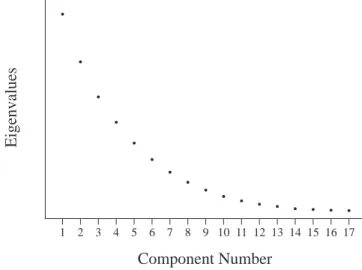
The break in the scree plot on page 3 of Output 1.1 was unusually obvious. In contrast, consider the plot that appears in Figure 1.2.
Eigenvalues
Component Number
1 2 3 4 5 6 7 8 9 10 11 12 13 14 15 16 17
Figure 1.2: A Scree Plot with No Obvious Break
Figure 1.2 presents a fictitious scree plot from a principal component analysis of 17 variables. Notice that there is no obvious break in the plot that separates the meaningful components from the trivial components. Most researchers would agree that components 1 and 2 are probably
meaningful, and that components 13–17 are probably trivial, but it is difficult to decide exactly where you should draw the line.
Scree plots such as the one presented in Figure 1.2 are common in social science research. When encountered, the use of the scree test must be supplemented with additional criteria, such as the variance accounted for criterion and the interpretability criterion, to be described later.
Why do they call it a “scree” test? The word “scree” refers to the loose rubble that lies at the base of a cliff. When performing a scree test, you normally hope that the scree plot will take the form of a cliff: At the top will be the eigenvalues for the few meaningful components, followed by a break (the edge of the cliff). At the bottom of the cliff will lie the scree: eigenvalues for the trivial components.
In some cases, a computer printer may not be able to prepare an eigenvalue plot with the degree of precision that is necessary to perform a sensitive scree test. In such cases, it may be best to prepare the plot by hand. This may be done simply by referring to the eigenvalue table on output page 2. Using the eigenvalues from this table, you can prepare an eigenvalue plot following the same format used by the SAS System (component numbers on the horizontal axis, eigenvalues on the vertical). Such a hand-drawn plot may make it easier to identify the break in the
eigenvalues, if one exists.
C. Proportion of variance accounted for. A third criterion in solving the number of factors problem involves retaining a component if it accounts for a specified proportion (or percentage) of variance in the data set. For example, you may decide to retain any component that accounts for at least 5% or 10% of the total variance. This proportion can be calculated with a simple formula:
Proportion = Eigenvalue for the component of interest
Total eigenvalues of the correlation matrix
In principal component analysis, the “total eigenvalues of the correlation matrix” is equal to the total number of variables being analyzed (because each variable contributes one unit of variance to the analysis).
Fortunately, it is not necessary to actually compute these percentages by hand, since they are provided in the results of PROC FACTOR. The proportion of variance accounted for by each component is printed in the eigenvalue table from output page 2, and appears to the right of the “Proportion” heading.
The eigenvalue table for the current analysis appears on page 2 of Output 1.1. From the
“Proportion” line in this eigenvalue table, you can see that the first component alone accounts for 38% of the total variance, the second component alone accounts for 33%, the third component
accounts for 13%, and the fourth component accounts for 7%. Assume that you have decided to retain any component that accounts for at least 10% of the total variance in the data set. For the present results, using this criterion would cause you to retain components 1, 2, and 3 (notice that use of this criterion would result in retaining more components than would be retained with the two preceding criteria).
An alternative criterion is to retain enough components so that the cumulative percent of variance accounted for is equal to some minimal value. For example, remember that components 1, 2, 3, and 4 accounted for approximately 38%, 33%, 13%, and 7% of the total variance, respectively. Adding these percentages together results in a sum of 91%. This means that the cumulative percent of variance accounted for by components 1, 2, 3, and 4 is 91%. When researchers use the “cumulative percent of variance accounted for” as the criterion for solving the number-of-components problem, they usually retain enough number-of-components so that the cumulative percent of variance accounted for at least 70% (and sometimes 80%).
With respect to the results of PROC FACTOR, the “cumulative percent of variance accounted for” is presented in the eigenvalue table (from page 2), to the right of the “Cumulative” heading. For the present analysis, this information appears in the eigenvalue table on page 2 of
Output 1.1. Notice the values that appear to the right of the heading “Cumulative”: Each value in this line indicates the percent of variance accounted for by the present component, as well as all preceding components. For example, the value for component 2 is .7068 (this appears at the intersection of the row headed “Cumulative” and the column headed “2”). This value of .7068 indicates that approximately 71% of the total variance is accounted for by components 1 and 2 combined. The corresponding entry for component 3 is .8397, meaning that approximately 84% of the variance is accounted for by components 1, 2, and 3 combined. If you were to use 70% as the “critical value” for determining the number of components to retain, you would retain
components 1 and 2 in the present analysis.
The proportion of variance criterion has a number of positive features. For example, in most cases, you would not want to retain a group of components that, combined, account for only a minority of the variance in the data set (say, 30%). Nonetheless, the critical values discussed earlier (10% for individual components and 70%-80% for the combined components) are obviously arbitrary. Because of these and related problems, this approach has sometimes been criticized for its subjectivity (Kim & Mueller, 1978b).
D. The interpretability criteria. Perhaps the most important criterion for solving the “number-of-components” problem is the interpretability criterion: interpreting the substantive meaning of the retained components and verifying that this interpretation makes sense in terms of what is known about the constructs under investigation. The following list provides four rules to follow in doing this. A later section (titled “Step 4: Interpreting the Rotated Solution”) shows how to actually interpret the results of a principal component analysis; the following rules will be more meaningful after you have completed that section.
1. Are there at least three variables (items) with significant loadings on each retained component? A solution is less satisfactory if a given component is measured by less than three variables.
2. Do the variables that load on a given component share the same conceptual meaning? For example, if three questions on a survey all load on component 1, do all three of these questions seem to be measuring the same construct?
3. Do the variables that load on different components seem to be measuring different constructs? For example, if three questions load on component 1, and three other questions load on component 2, do the first three questions seem to be measuring a construct that is conceptually different from the construct measured by the last three questions?
4. Does the rotated factor pattern demonstrate “simple structure?” Simple structure means that the pattern possesses two characteristics: (a) Most of the variables have
relatively high factor loadings on only one component, and near zero loadings on the other components, and (b) most components have relatively high factor loadings for some variables, and near-zero loadings for the remaining variables. This concept of simple structure will be explained in more detail in a later section titled “Step 4: Interpreting the Rotated Solution.”
Recommendations. Given the preceding options, what procedure should you actually follow in solving the number-of-components problem? We recommend combining all four in a structured sequence. First, use the MINEIGEN=1 options to implement the eigenvalue-one criterion. Review this solution for interpretability, and use caution if the break between the components with eigenvalues above 1.00 and those below 1.00 is not clear-cut (i.e., if component 2 has an eigenvalue of 1.001, and component 2 has an eigenvalue of 0.998).
Next, perform a scree test and look for obvious breaks in the eigenvalues. Because there will often be more than one break in the scree plot, it may be necessary to examine two or more possible solutions.
Next, review the amount of common variance accounted for by each individual component. You probably should not rigidly use some specific but arbitrary cutoff point such as 5% or 10%. Still, if you are retaining components that account for as little as 2% or 4% of the variance, it may be wise to take a second look at the solution and verify that these latter components are of truly substantive importance. In the same way, it is best if the combined components account for at least 70% of the cumulative variance; if less than 70% is accounted for, it may be wise to consider alternative solutions that include a larger number of components.
Finally, apply the interpretability criteria to each solution that is examined. If more than one solution can be justified on the basis of the preceding criteria, which of these solutions is the most interpretable? By seeking a solution that is both interpretable and also satisfies one (or more) of the other three criteria, you maximize chances of retaining the correct number of components.
Step 3: Rotation to a Final Solution
Factor patterns and factor loadings. After extracting the initial components, PROC FACTOR will create an unrotated factor pattern matrix. The rows of this matrix represent the variables being analyzed, and the columns represent the retained components (these components are referred to as FACTOR1, FACTOR2 and so forth in the output).
The entries in the matrix are factor loadings. A factor loading is a general term for a coefficient that appears in a factor pattern matrix or a factor structure matrix. In an analysis that results in oblique (correlated) components, the definition for a factor loading is different depending on whether it is in a factor pattern matrix or in a factor structure matrix. However, the situation is simpler in an analysis that results in orthogonal components (as in the present chapter): In an orthogonal analysis, factor loadings are equivalent to bivariate correlations between the observed variables and the components.
For example, the factor pattern matrix from the current analysis appears on page 4 of
Output 1.1. Where the rows for observed variables intersect with the column for FACTOR1, you can see that the correlation between V1 and the first component is .58; the correlation between V2 and the first component is .48, and so forth.
Rotations. Ideally, you would like to review the correlations between the variables and the components and use this information to interpret the components; that is, to determine what construct seems to be measured by component 1, what construct seems to be measured by component 2, and so forth. Unfortunately, when more than one component has been retained in an analysis, the interpretation of an unrotated factor pattern is usually quite difficult. To make interpretation easier, you will normally perform an operation called a rotation. A rotation is a linear transformation that is performed on the factor solution for the purpose of making the solution easier to interpret.
PROC FACTOR allows you to request several different types of rotations. The preceding program that analyzed data from the POI study included the statement
ROTATE=VARIMAX
which requests a varimax rotation. A varimax rotation is an orthogonal rotation, meaning that it results in uncorrelated components. Compared to some other types of rotations, a varimax rotation tends to maximize the variance of a column of the factor pattern matrix (as opposed to a row of the matrix). This rotation is probably the most commonly used orthogonal rotation in the social sciences. The results of the varimax rotation for the current analysis appear on page 5 of Output 1.1.
Step 4: Interpreting the Rotated Solution
Interpreting a rotated solution means determining just what is measured by each of the retained components. Briefly, this involves identifying the variables that demonstrate high loadings for a
given component, and determining what these variables have in common. Usually, a brief name is assigned to each retained component that describes its content.
The first decision to be made at this stage is to decide how large a factor loading must be to be considered “large.” Stevens (1986) discusses some of the issues relevant to this decision, and even provides guidelines for testing the statistical significance of factor loadings. Given that this is an introductory treatment of principal component analysis, however, simply consider a loading to be “large” if its absolute value exceeds .40.
The rotated factor pattern for the POI study appears on page 5 of Output 1.1. The following text provides a structured approach for interpreting this factor pattern.
A. Read across the row for the first variable . All “meaningful loadings” (i.e., loadings greater than .40) have been flagged with an asterisk (“*”). This was accomplished by including the FLAG=.40 option in the preceding program. If a given variable has a meaningful loading on more than one component, scratch that variable out and ignore it in your interpretation. In many situations, researchers want to drop variables that load on more than one component, because the variables are not pure measures of any one construct. In the present case, this means looking at the row headed “V1”, and reading to the right to see if it loads on more than one component. In this case it does not, so you may retain this variable.
B. Repeat this process for the remaining variables, scratching out any variable that loads on more than one component. In this analysis, none of the variables have high loadings on more than one component, so none will have to be dropped.
C. Review all of the surviving variables with high loadings on component 1 to determine the nature of this component. From the rotated factor pattern, you can see that only items 4, 5, and 6 load on component 1 (note the asterisks). It is now necessary to turn to the questionnaire itself and review the content of the questions in order to decide what a given component should be named. What do questions 4, 5, and 6 have in common? What common construct do they seem to be measuring? For illustration, the questions being analyzed in the present case are reproduced here. Remember that question 4 was represented as V4 in the SAS program, question 5 was V5, and so forth. Read questions 4, 5, and 6 to see what they have in common.
1 2 3 4 5 6 7 1. Went out of my way to do a favor for a coworker.
1 2 3 4 5 6 7 2. Went out of my way to do a favor for a relative.
1 2 3 4 5 6 7 3. Went out of my way to do a favor for a friend.
1 2 3 4 5 6 7 4. Gave money to a religious charity.
1 2 3 4 5 6 7 5. Gave money to a charity not associated with a religion.
1 2 3 4 5 6 7 6. Gave money to a panhandler.
Questions 4, 5, and 6 all seem to deal with “giving money to the needy.” It is therefore reasonable to label component 1 the “financial giving” component.
D. Repeat this process to name the remaining retained components. In the present case, there is only one remaining component to name: component 2. This component has high loadings for questions 1, 2, and 3. In reviewing these items, it becomes clear that each seems to deal with helping friends, relatives, or other acquaintances. It is therefore appropriate to name this the “acquaintance helping” component.
E. Determine whether this final solution satisfies the interpretability criteria. An earlier section indicated that the overall results of a principal component analysis are satisfactory only if they meet a number of interpretability criteria. In the following list, the adequacy of the rotated factor pattern presented on page 5 of Output 1.1 is assessed in terms of these criteria.
1. Are there at least three variables (items) with significant loadings on each retained component? In the present example, three variables loaded on component 1, and three also loaded on component 2, so this criterion was met.
2. Do the variables that load on a given component share some conceptual meaning? All three variables loading on component 1 are clearly measuring giving to the needy, while all three loading on component 2 are clearly measuring prosocial acts performed for acquaintances. Therefore, this criterion is met.
3. Do the variables that load on different components seem to be measuring different constructs? The items loading on component 1 clearly are measuring the respondents’ financial contributions, while the items loading on component 2 are clearly measuring helpfulness toward acquaintances. Because these seem to be conceptually very different constructs, this criterion seems to be met as well.
4. Does the rotated factor pattern demonstrate “simple structure?” Earlier, it was said that a rotated factor pattern demonstrates simple structure when it has two
characteristics. First, most of the variables should have high loadings on one
component, and near-zero loadings on the other components. It can be seen that the pattern obtained here meets that requirement: items 1-3 have high loadings on
component 2, and near-zero loadings on component 1. Similarly, items 4-6 have high loadings on component 1, and near-zero loadings on component 2. The second
characteristic of simple structure is that each component should have high loadings for some variables, and near-zero loadings for the others. Again, the pattern obtained here also meets this requirement: component 1 has high loadings for items 4-6 and near-zero loadings for the other items, while component 2 has high loadings for items 1-3, and near-zero loadings on the remaining items. In short, the rotated component pattern obtained in this analysis does seem to demonstrate simple structure.
Step 5: Creating Factor Scores or Factor-Based Scores
Once the analysis is complete, it is often desirable to assign scores to each subject to indicate where that subject stands on the retained components. For example, the two components retained in the present study were interpreted as a financial giving component and an acquaintance helping component. You may want to now assign one score to each subject to indicate that subject’s standing on the financial giving component, and a different score to indicate that subject’s standing on the acquaintance helping component. With this done, these component scores could be used either as predictor variables or as criterion variables in subsequent analyses.
Before discussing the options for assigning these scores, it is important to first draw a distinction between factor scores versus factor-based scores. In principal component analysis, a factor score (or component score) is a linear composite of the optimally-weighted observed variables. If requested, PROC FACTOR will compute each subject’s factor scores for the two components by
• determining the optimal regression weights
• multiplying subject responses to the questionnaire items by these weights • summing the products.
The resulting sum will be a given subject’s score on the component of interest. Remember that a separate equation, with different weights, is developed for each retained component.
A factor-based score, on the other hand, is merely a linear composite of the variables that demonstrated meaningful loadings for the component in question. For example, in the preceding analysis, items 4, 5, and 6 demonstrated meaningful loadings for the financial giving component. Therefore, you could calculate the factor-based score on this component for a given subject by simply adding together his or her responses to items 4, 5, and 6. Notice that, with a factor-based score, the observed variables are not multiplied by optimal weights before they are summed.