Return of the Devil in the Details: Delving Deep into Convolutional Nets

CHATFIELD ET AL.: RETURN OF THE DEVIL

Return of the Devil in the Details:

Delving Deep into Convolutional Nets

[email protected] Karen Simonyan [email protected] Andrea Vedaldi [email protected] Andrew Zisserman [email protected]

Visual Geometry Group

Department of Engineering Science University of Oxford

Oxford, UK

Abstract

The latest generation of Convolutional Neural Networks (CNN) have achieved im-pressive results in challenging benchmarks on image recognition and object detection, significantly raising the interest of the community in these methods. Nevertheless, it is still unclear how different CNN methods compare with each other and with previ-ous state-of-the-art shallow representations such as the Bag-of-Visual-Words and the Improved Fisher Vector. This paper conducts a rigorous evaluation of these new tech-niques, exploring different deep architectures and comparing them on a common ground, identifying and disclosing important implementation details. We identify several useful properties of CNN-based representations, including the fact that the dimensionality of the CNN output layer can be reduced significantly without having an adverse effect on performance. We also identify aspects of deep and shallow methods that can be success-fully shared. In particular, we show that the data augmentation techniques commonly applied to CNN-based methods can also be applied to shallow methods, and result in an analogous performance boost. Source code and models to reproduce the experiments in the paper is made publicly available.

1

Introduction

Perhaps the single most important design choice in current state-of-the-art image classifica-tion and object recogniclassifica-tion systems is the choice of visual features, or image representaclassifica-tion. In fact, most of the quantitative improvements to image understanding obtained in the past dozen years can be ascribed to the introduction of improved representations, from the Bag-of-Visual-Words(BoVW) [6,28] to the (Improved) Fisher Vector(IFV) [23]. A common characteristic of these methods is that they are largelyhandcrafted. They are also relatively simple, comprising dense sampling of local image patches, describing them by means of visual descriptors such as SIFT, encoding them into a high-dimensional representation, and then pooling over the image. Recently, these handcrafted approaches have been substantially outperformed by the introduction of the latest generation ofConvolutional Neural Networks (CNNs) [19] to the computer vision field. These networks have a substantially more so-phisticated structure than standard representations, comprising several layers of non-linear

c

2014. The copyright of this document resides with its authors. It may be distributed unchanged freely in print or electronic forms.

CHATFIELD ET AL.: RETURN OF THE DEVIL feature extractors, and are therefore said to bedeep(in contrast, classical representation will be referred to asshallow). Furthermore, while their structure is handcrafted, they contain a very large number of parameters learnt from data. When applied to standard image classifi-cation and object detection benchmark datasets such as ImageNet ILSVRC [7] and PASCAL VOC [9] such networks have demonstrated excellent performance [8,11,20,25,27], signif-icantly better than standard image encodings [3].

Despite these impressive results, it remains unclear how different deep architectures com-pare to each other and to shallow computer vision methods such as IFV. Most papers did not test these representations extensively on a common ground, so a systematic evaluation of the effect of different design and implementation choices remains largely missing. As noted in our previous work [3], which compared the performance of various shallow visual encod-ings, theperformance of computer vision systems depends significantly on implementation details. For example, state-of-the-art methods such as [17] not only involve the use of a CNN, but also include other improvements such as the use of very large scale datasets, GPU computation, and data augmentation (also known as data jittering or virtual sampling). These improvements could also transfer to shallow representations such as the IFV, potentially ex-plaining a part of the performance gap [22].

In this study we analyse and empirically clarify these issues, conducting a large set of rigorous experiments (Sect.4), in many ways picking up the story where it last ended in [3] with the comparison of shallow encoders. We focus on methods to constructimage rep-resentations,i.e. encoding functionsφ mapping an imageIto a vectorφ(I)∈Rd suitable for analysis with a linear classifier, such as an SVM. We considerthree scenarios(Sect.2, Sect.3): shallow image representations, deep representations pre-trained on outside data, and deep representation pre-trained and then fine-tuned on the target dataset. As part of our tests, we exploregenerally-applicable best practicesthat are nevertheless more often found in combination with CNNs [17] or, alternatively, with shallow encoders [3], porting them with mutual benefit. These are (Sect.2): the use ofcolour information, feature normal-isation, and, most importantly, the use ofsubstantial data augmentation. We also determine scenario-specific best-practices, improving the ones in [3,24] and others, including dimen-sionality reduction for deep features. Finally, we achieveperformance competitive with the state of the art [21,30]on PASCAL VOC classification using less additional training data and significantly simpler techniques. As in [3], the source code and models to reproduce all experiments in this paper is available on the project website1.

2

Scenarios

This section introduces the three types of image representationφ(I)considered in this paper, describing them within the context of three different scenarios. Having outlined details spe-cific to each, general methodologies which apply to all three scenarios are reviewed, such as data augmentation and feature normalisation, together with the linear classifier (trained with a standard hinge loss). We also specify here the benchmark datasets used in the evaluation. Scenario 1: Shallow representation (IFV).Our reference shallow image representation is the IFV [23]. Our choice is motivated by the fact that IFV usually outperforms related encoding methods such as BoVW, LLC [3], and VLAD [15]. Given an imageI, the IFV φFV(I)is obtained by extracting a dense collection of patches and corresponding local de-scriptorsxi∈RD (e.g. SIFT) from the image at multiple scales. Each descriptorxiis then soft-quantized using a Gaussian Mixture Model withKcomponents. First and second order differences between each descriptorx_i and its Gaussian cluster mean µk are accumulated

CHATFIELD ET AL.: RETURN OF THE DEVIL

in corresponding blocksuk,vk in the vectorφFV(I)∈R2KD, appropriately weighed by the Gaussian soft-assignments and covariance, leading to a 2KD-dimensional image represen-tation φFV(I) = [u>1,v>1, . . .u>K,v>K]>. The improvedversion of the Fisher vector involves post-processingφFVby computing the signed square-root of its scalar components and nor-malising the result to a unit`2norm. The details of this construction can be found in [23]; here we follow the notation of [3].

Scenario 2: Deep representation (CNN) with pre-training. Our deep representations are inspired by the success of the CNN of Krizhevskyet al. [17]. As shown in [8,32], the vector of activitiesφCNN(I)of the penultimate layer of a deep CNN, learnt on a large dataset such as ImageNet [7], can be used as a powerful image descriptor applicable to other datasets. Numerous CNN architectures that improve the previous state of the art obtained using shal-low representations have been proposed, but choosing the best one remains an open question. Many are inspired by [17]: DeCAF [8,11], Caffe [16], Oquabet al. [20]. Others use larger networks with a smaller stride of the first convolutional layer: Zeiler and Fergus [32] and OverFeat [25,27]. Other differences include the CNN pre-training protocols. Here we adopt a single learning framework and experiment with architectures of different complexity ex-ploring their performance-speed trade-off.

Scenario 3: Deep representation (CNN) with pre-training and fine-tuning.In Scenario 2 features are trained on one (large) dataset and applied to another (usually smaller). How-ever, it was demonstrated [11] that fine-tuning a pre-trained CNN on the target data can significantly improve the performance. We consider this scenario separately from that of Scenario 2, as the image features become dataset-specific after the fine-tuning.

Data augmentation. Data augmentation is a method applicable to shallow and deep repre-sentations, but that has been so far mostly applied to the latter [17,32]. By augmentation we mean perturbing an imageI by transformations that leave the underlying class unchanged (e.g. cropping and flipping) in order to generate additional examples of the class. Augmenta-tion can be applied at training time, at test time, or both. The augmented samples can either be taken as-is or combined to form a single feature, e.g. using sum/max-pooling or stacking. Linear predictors. All the representationsφ(I)in the three scenarios are used to construct linear predictorshw,φ(I)ifor each class to be recognized. These predictors are learnt using Support Vector Machines (SVM) by fittingwto the available training data by minimizing an objective function balancing a quadratic regularizer and the hinge-loss. The parameterCin the SVM, trading-off regularizer and loss, is determined using an held-off validation subset of the data. Here we use the same learning framework with all representations. It is common experience that linear classifiers are particularly sensitive to thenormalisation of the data and that, in particular, SVMs tend to benefit from`2normalisation [23] (an interpretation is that after normalisation the inner product corresponds to the cosine similarly).

Benchmark data. As reference benchmark we use the PASCAL VOC [9] data as already done in [3]. TheVOC-2007edition contains about 10,000 images split into train, valida-tion, and test sets, and labelled with twenty object classes. A one-vs-rest SVM classifier for each class is learnt and evaluated independently and the performance is measured as mean Average Precision (mAP) across all classes. TheVOC-2012edition contains roughly twice as many images and does not include test labels; instead, evaluation uses the official PAS-CAL Evaluation Server. To train deep representations we use theILSVRC-2012challenge dataset. This contains 1,000 object categories from ImageNet [7] with roughly 1.2M training images, 50,000 validation images, and 100,000 test images. Performance is evaluated using the top-5 classification error. Finally, we also evaluate over theCaltech-101and

Caltech-CHATFIELD ET AL.: RETURN OF THE DEVIL 256image classification benchmarks [10,12]. For Caltech-101, we followed the protocol of [3], and considered three random splits into training and testing data, each of which com-prises 30 training and up to 30 testing images per class. For Caltech-256, two random splits were generated, each of which contains 60 training images per class, and the rest are used for testing. On both Caltech datasets, performance is measured using mean class accuracy.

3

Details

3.1

Improved Fisher Vector details

Our IFV representation uses a slightly improved setting compared to the best result of [3]. Computation starts by upscaling the image I by a factor of 2 [26], followed by SIFT features extraction with a stride of 3 pixels at 7 different scales with√2 scale increments. These features are square-rooted as suggested by [1], and decorrelated and reduced in di-mension from 128Dto 80Dusing PCA. A GMM withK=256 components is learnt from features sampled from the training images. Hence the Fisher VectorφFV(I) has dimen-sion 2KD=40,960. Before use in classification, the vector is signed-square-rooted and l2-normalised (square rooting correspond to the Hellinger’s kernel map [29]). As in [3], square-rooting is applied twice, once to the raw encodings, and once again after sum pooling and normalisation. In order to capture weak geometrical information, the IFV representa-tion is used in aspatial pyramid[18]. As in [3], the image is divided into 1×1, 3×1, and 2×2 spatial subdivisions and corresponding IFVs are computed and stacked with an overall dimension of 8×2KD=327,680 elements.

In addition to this standard formulation, we experiment with a few modifications. The first one is the use ofintra-normalisationof the descriptor blocks, an idea recently proposed for the VLAD descriptor [2]. In this case, the`2normalisation is applied to the individual sub-blocks(uk,vk)of the vectorφFV(I), which helps to alleviate the local feature bursti-ness [14]. In the case of the improved intra-normalised features, it was found that applying the square-rooting only once to the final encoding produced the best results.

The second modification is the use ofspatially-extended local descriptors[26] instead of a spatial pyramid. Here descriptorsxiare appended with their image location(xi,yi)before quantization with the GMM. Formally,xi is extended, after PCA projection, with its nor-malised spatial coordinates:[x>_i ,xi/W−0.5,yi/H−0.5]>, whereW×Hare the dimensions of the image. Since the GMM quantizes both appearance and location, this allows for spatial information to be captured directly by the soft-quantization process. This method is signif-icantly more memory-efficient than using a spatial pyramid. Specifically, the PCA-reduced SIFT features are spatially augmented by appending(x,y)yieldingD=82 dimensional de-scriptors pooled in a 2KD=41,984 dimensional IFV.

The third modification is the use of colour features in addition to SIFT descriptors. While colour information is used in CNNs [17] and by the original FV paper [23], it was not explored in our previous comparison [3]. We do so here by adopting the same Local Colour Statistics (LCS) features as used by [23]. LCS is computed by dividing an input patch into a 4×4 spatial grid (akin to SIFT), and computing the mean and variance of each of theLab colour channels for each cell of the grid. The LCS dimensionality is thus 4×4×2×3=96. This is then encoded in a similar manner to SIFT.

3.2

Convolutional neural networks details

The CNN-based features are based on three CNN architectures representative of the state of the art (shown in Table1) each exploring a different accuracy/speed trade-off. To ensure a fair comparison between them, these networks are trained using the same training protocol

CHATFIELD ET AL.: RETURN OF THE DEVIL

Arch. conv1 conv2 conv3 conv4 conv5 full6 full7 full8 CNN-F

64x11x11 256x5x5 256x3x3 256x3x3 256x3x3 4096 4096 1000 st. 4, pad 0 st. 1, pad 2 st. 1, pad 1 st. 1, pad 1 st. 1, pad 1 drop- drop- soft-LRN, x2 pool soft-LRN, x2 pool - - x2 pool out out max CNN-M

96x7x7 256x5x5 512x3x3 512x3x3 512x3x3 4096 4096 1000 st. 2, pad 0 st. 2, pad 1 st. 1, pad 1 st. 1, pad 1 st. 1, pad 1 drop- drop- soft-LRN, x2 pool soft-LRN, x2 pool - - x2 pool out out max CNN-S

96x7x7 256x5x5 512x3x3 512x3x3 512x3x3 4096 4096 1000 st. 2, pad 0 st. 1, pad 1 st. 1, pad 1 st. 1, pad 1 st. 1, pad 1 drop- drop- soft-LRN, x3 pool x2 pool - - x3 pool out out max Table 1: CNN architectures. Each architecture contains 5 convolutional layers (conv 1–5) and three fully-connected layers (full 1–3). The details of each of the convolutional layers are given in three sub-rows: the first specifies the number of convolution filters and their receptive field size as “num x size x size”; the second indicates the convolution stride (“st.”) and spatial padding (“pad”); the third indicates if Local Response Normalisation (LRN) [17] is applied, and the max-pooling downsampling factor. For full 1–3, we specify their dimen-sionality, which is the same for all three architectures. Full6 and full7 are regularised using dropout [17], while the last layer acts as a multi-way soft-max classifier. The activation func-tion for all weight layers (except for full8) is the REctificafunc-tion Linear Unit (RELU) [17]. and the same implementation, which we developed based on the open-source Caffe frame-work [16]. `2-normalising the CNN featuresφCNN(I)before use in the SVM was found to be important for performance.

OurFast (CNN-F)architecture is similar to the one used by Krizhevskyet al. [17]. It comprises 8 learnable layers, 5 of which are convolutional, and the last 3 are fully-connected. The input image size is 224×224. Fast processing is ensured by the 4 pixel stride in the first convolutional layer. The main differences between our architecture and that of [17] are the reduced number of convolutional layers and the dense connectivity between convolutional layers ([17] used sparse connections to enable training on two GPUs).

OurMedium (CNN-M)architecture is similar to the one used by Zeiler and Fergus [32]. It is characterised by the decreased stride and smaller receptive field of the first convolutional layer, which was shown to be beneficial on the ILSVRC dataset. At the same time, conv2 uses larger stride (2 instead of 1) to keep the computation time reasonable. The main differ-ence between our net and that of [32] is we use less filters in the conv4 layer (512vs. 1024). OurSlow (CNN-S)architecture is related to the ‘accurate’ network from the OverFeat package [27]. It also uses 7×7 filters with stride 2 in conv1. Unlike CNN-M and [32], the stride in conv2 is smaller (1 pixel), but the max-pooling window in conv1 and conv5 is larger (3×3) to compensate for the increased spatial resolution. Compared to [27], we use 5 convolutional layers as in the previous architectures ([27] used 6), and less filters in conv5 (512 instead of 1024); we also incorporate an LRN layer after conv1 ([27] did not use contrast normalisation).

CNN training. In general, our CNN training procedure follows that of [17], learning on ILSVRC-2012 using gradient descent with momentum. The hyper-parameters are the same as used by [17]: momentum 0.9; weight decay 5·10−4; initial learning rate 10−2, which is decreased by a factor of 10, when the validation error stop decreasing. The layers are initialised from a Gaussian distribution with a zero mean and variance equal to 10−2_{. We} also employ similar data augmentation in the form of random crops, horizontal flips, and RGB colour jittering. Test time crop sampling is discussed in Sect.3.3; at training time, 224×224 crops are sampled randomly, rather than deterministically. Thus, the only notable difference to [17] is that the crops are taken from the whole training imageP×256,P≥256,

CHATFIELD ET AL.: RETURN OF THE DEVIL rather than its 256×256 centre. Training was performed on a single NVIDIA GTX Titan GPU and the training time varied from 5 days for CNN-F to 3 weeks for CNN-S.

CNN fine-tuning on the target dataset. In our experiments, we fine-tuned CNN-S using VOC-2007, VOC-2012, or Caltech-101 as the target data. Fine-tuning was carried out us-ing the same framework (and the same data augmentation), as we used for CNN trainus-ing on ILSVRC. The last fully-connected layer (conv8) has output dimensionality equal to the number of classes, which differs between datasets, so we initialised it from a Gaussian distri-bution (as used for CNN training above). Now we turn to dataset-specific fine-tuning details. VOC-2007 and VOC-2012. Considering that PASCAL VOC is a multi-label dataset (i.e. a single image might have multiple labels), we replaced the softmax regression loss with a more appropriate loss function, for which we considered two options: one-vs-rest classifi-cation hinge loss (the same loss as used in the SVM experiments) and ranking hinge loss. Both losses define constraints on the scores of positive (Ipos) and negative (Ineg) images for each class: wcφ(Ipos)>1−ξ,wcφ(Ineg)<−1+ξ for the classification loss,wcφ(Ipos)>

wcφ(Ineg) +1−ξ for the ranking loss (wcis thec-th row of the last fully-connected layer, which can be seen as a linear classifier on deep featuresφ(I);ξ is a slack variable). Our fine-tuned networks are denoted as “CNN S TUNE-CLS” (for the classification loss) and “CNN S TUNE-RNK” (for the ranking loss). In the case of both VOC datasets, the training and validation subsets were combined to form a single training set. Given the smaller size of the training data when compared to ILSVRC-2012, we controlled for over-fitting by using lower initial learning rates for the fine-tuned hidden layers. The learning rate schedule for the last layer / hidden layers was: 10−2/10−4→10−3/10−4→10−4/10−4→10−5/10−5. Caltech-101 dataset contains a single class label per image, so fine-tuning was performed using the softmax regression loss. Other settings (including the learning rate schedule) were the same as used for the VOC fine-tuning experiments.

Low-dimensional CNN feature training. Our baseline networks (Table1) have the same dimensionality of the last hidden layer (full7): 4096. This design choice is in accordance with the state-of-the-art architectures [17,27,32], and leads to a 4096-D dimensional image representation, which is already rather compact compared to IFV. We further trained three modifications of the CNN-M network, with lower dimensional full7 layers of: 2048, 1024, and 128 dimensions respectively. The networks were learnt on ILSVRC-2012. To speed-up training, all layers aside from full7/full8 were set to those of the CNN-M net and a lower initial learning rate of 10−3was used. The initial learning rate of full7/full8 was set to 10−2.

3.3

Data augmentation details

We explore three data augmentation strategies. The first strategy is to useno augmentation. In contrast to IFV, however, CNNs require images to be transformed to a fixed size (224×

224) even when no augmentation is used. Hence the image is downsized so that the smallest dimension is equal to 224 pixels and a 224×224 crop is extracted from the centre.2 The second strategy is to useflip augmentation, mirroring images about they-axis producing two samples from each image. The third strategy, termedC+F augmentation, combines cropping and flipping. For CNN-based representations, the image is downsized so that the smallest dimension is equal to 256 pixels. Then 224×224 crops are extracted from the four corners and the centre of the image. Note that the crops are sampled from the whole image, rather than its 256×256 centre, as done by [17]. These crops are then flipped about the y-axis, producing 10 perturbed samples per input image. In the case of the IFV encoding,

CHATFIELD ET AL.: RETURN OF THE DEVIL Method SPool Image Aug. Dim mAP

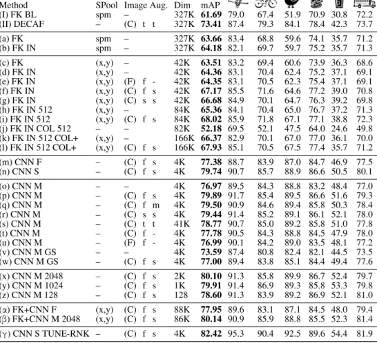
(I) FK BL spm – 327K 61.69 79.0 67.4 51.9 70.9 30.8 72.2 (II) DECAF – (C) t t 327K 73.41 87.4 79.3 84.1 78.4 42.3 73.7 (a) FK spm – 327K 63.66 83.4 68.8 59.6 74.1 35.7 71.2 (b) FK IN spm – 327K 64.18 82.1 69.7 59.7 75.2 35.7 71.3 (c) FK (x,y) – 42K 63.51 83.2 69.4 60.6 73.9 36.3 68.6 (d) FK IN (x,y) – 42K 64.36 83.1 70.4 62.4 75.2 37.1 69.1 (e) FK IN (x,y) (F) f - 42K 64.35 83.1 70.5 62.3 75.4 37.1 69.1 (f) FK IN (x,y) (C) f s 42K 67.17 85.5 71.6 64.6 77.2 39.0 70.8 (g) FK IN (x,y) (C) s s 42K 66.68 84.9 70.1 64.7 76.3 39.2 69.8 (h) FK IN 512 (x,y) – 84K 65.36 84.1 70.4 65.0 76.7 37.2 71.3 (i) FK IN 512 (x,y) (C) f s 84K 68.02 85.9 71.8 67.1 77.1 38.8 72.3 (j) FK IN COL 512 – – 82K 52.18 69.5 52.1 47.5 64.0 24.6 49.8 (k) FK IN 512 COL+ (x,y) – 166K 66.37 82.9 70.1 67.0 77.0 36.1 70.0 (l) FK IN 512 COL+ (x,y) (C) f s 166K 67.93 85.1 70.5 67.5 77.4 35.7 71.2 (m) CNN F – (C) f s 4K 77.38 88.7 83.9 87.0 84.7 46.9 77.5 (n) CNN S – (C) f s 4K 79.74 90.7 85.7 88.9 86.6 50.5 80.1 (o) CNN M – – 4K 76.97 89.5 84.3 88.8 83.2 48.4 77.0 (p) CNN M – (C) f s 4K 79.89 91.7 85.4 89.5 86.6 51.6 79.3 (q) CNN M – (C) f m 4K 79.50 90.9 84.6 89.4 85.8 50.3 78.4 (r) CNN M – (C) s s 4K 79.44 91.4 85.2 89.1 86.1 52.1 78.0 (s) CNN M – (C) t t 41K 78.77 90.7 85.0 89.2 85.8 51.0 77.8 (t) CNN M – (C) f - 4K 77.78 90.5 84.3 88.8 84.5 47.9 78.0 (u) CNN M – (F) f - 4K 76.99 90.1 84.2 89.0 83.5 48.1 77.2 (v) CNN M GS – – 4K 73.59 87.4 80.8 82.4 82.1 44.5 73.5 (w) CNN M GS – (C) f s 4K 77.00 89.4 83.8 85.1 84.4 49.4 77.6 (x) CNN M 2048 – (C) f s 2K 80.10 91.3 85.8 89.9 86.7 52.4 79.7 (y) CNN M 1024 – (C) f s 1K 79.91 91.4 86.9 89.3 85.8 53.3 79.8 (z) CNN M 128 – (C) f s 128 78.60 91.3 83.9 89.2 86.9 52.1 81.0 (α) FK+CNN F (x,y) (C) f s 88K 77.95 89.6 83.1 87.1 84.5 48.0 79.4 (β) FK+CNN M 2048 (x,y) (C) f s 86K 80.14 90.9 85.9 88.8 85.5 52.3 81.4 (γ) CNN S TUNE-RNK – (C) f s 4K 82.42 95.3 90.4 92.5 89.6 54.4 81.9

Table 2: VOC 2007 results(continued overleaf). See Sect.4for details. the same crops are extracted, but at the original image resolution.

4

Analysis

This section describes the experimental results, comparing different features and data aug-mentation schemes. The results are given in Table 2 for VOC-2007 and analysed next, starting from generally applicable methods such as augmentation and then discussing the specifics of each scenario. We then move onto other datasets and the state of the art in Sect.4. Data augmentation. We experiment with no data augmentation (denotedImage Aug=–in Tab. 2), flip augmentation (Image Aug=F), and C+F augmentation (Image Aug=C). Aug-mented images are used as stand-alone samples (f), or by fusing the corresponding descrip-tors using sum (s) or max (m) pooling or stacking (t). So for exampleImage Aug=(C) f s in row[f]of Tab.2means that C+F augmentation is used to generate additional samples in training (f), and is combined with sum-pooling in testing (s).

Augmentation consistently improves performance by∼3% for both IFV (e.g.[d]vs.[f]) and CNN (e.g.[o]vs.[p]). Using additional samples for training and sum-pooling for testing works best ([p]) followed by sum-pooling[r], max pooling[q], and stacking[s]. In terms of the choice of transformations, flipping improves only marginally ([o]vs.[u]), but using the more expensive C+F sampling improves, as seen, by about 2∼3% ([o] vs.[p]). We experimented with sampling more transformations, taking a higher density of crops from the

CHATFIELD ET AL.: RETURN OF THE DEVIL

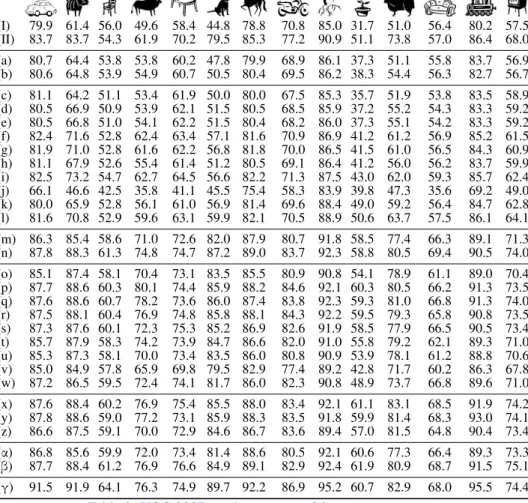
(I) 79.9 61.4 56.0 49.6 58.4 44.8 78.8 70.8 85.0 31.7 51.0 56.4 80.2 57.5 (II) 83.7 83.7 54.3 61.9 70.2 79.5 85.3 77.2 90.9 51.1 73.8 57.0 86.4 68.0 (a) 80.7 64.4 53.8 53.8 60.2 47.8 79.9 68.9 86.1 37.3 51.1 55.8 83.7 56.9 (b) 80.6 64.8 53.9 54.9 60.7 50.5 80.4 69.5 86.2 38.3 54.4 56.3 82.7 56.7 (c) 81.1 64.2 51.1 53.4 61.9 50.0 80.0 67.5 85.3 35.7 51.9 53.8 83.5 58.9 (d) 80.5 66.9 50.9 53.9 62.1 51.5 80.5 68.5 85.9 37.2 55.2 54.3 83.3 59.2 (e) 80.5 66.8 51.0 54.1 62.2 51.5 80.4 68.2 86.0 37.3 55.1 54.2 83.3 59.2 (f) 82.4 71.6 52.8 62.4 63.4 57.1 81.6 70.9 86.9 41.2 61.2 56.9 85.2 61.5 (g) 81.9 71.0 52.8 61.6 62.2 56.8 81.8 70.0 86.5 41.5 61.0 56.5 84.3 60.9 (h) 81.1 67.9 52.6 55.4 61.4 51.2 80.5 69.1 86.4 41.2 56.0 56.2 83.7 59.9 (i) 82.5 73.2 54.7 62.7 64.5 56.6 82.2 71.3 87.5 43.0 62.0 59.3 85.7 62.4 (j) 66.1 46.6 42.5 35.8 41.1 45.5 75.4 58.3 83.9 39.8 47.3 35.6 69.2 49.0 (k) 80.0 65.9 52.8 56.1 61.0 56.9 81.4 69.6 88.4 49.0 59.2 56.4 84.7 62.8 (l) 81.6 70.8 52.9 59.6 63.1 59.9 82.1 70.5 88.9 50.6 63.7 57.5 86.1 64.1 (m) 86.3 85.4 58.6 71.0 72.6 82.0 87.9 80.7 91.8 58.5 77.4 66.3 89.1 71.3 (n) 87.8 88.3 61.3 74.8 74.7 87.2 89.0 83.7 92.3 58.8 80.5 69.4 90.5 74.0 (o) 85.1 87.4 58.1 70.4 73.1 83.5 85.5 80.9 90.8 54.1 78.9 61.1 89.0 70.4 (p) 87.7 88.6 60.3 80.1 74.4 85.9 88.2 84.6 92.1 60.3 80.5 66.2 91.3 73.5 (q) 87.6 88.6 60.7 78.2 73.6 86.0 87.4 83.8 92.3 59.3 81.0 66.8 91.3 74.0 (r) 87.5 88.1 60.4 76.9 74.8 85.8 88.1 84.3 92.2 59.5 79.3 65.8 90.8 73.5 (s) 87.3 87.6 60.1 72.3 75.3 85.2 86.9 82.6 91.9 58.5 77.9 66.5 90.5 73.4 (t) 85.7 87.9 58.3 74.2 73.9 84.7 86.6 82.0 91.0 55.8 79.2 62.1 89.3 71.0 (u) 85.3 87.3 58.1 70.0 73.4 83.5 86.0 80.8 90.9 53.9 78.1 61.2 88.8 70.6 (v) 85.0 84.9 57.8 65.9 69.8 79.5 82.9 77.4 89.2 42.8 71.7 60.2 86.3 67.8 (w) 87.2 86.5 59.5 72.4 74.1 81.7 86.0 82.3 90.8 48.9 73.7 66.8 89.6 71.0 (x) 87.6 88.4 60.2 76.9 75.4 85.5 88.0 83.4 92.1 61.1 83.1 68.5 91.9 74.2 (y) 87.8 88.6 59.0 77.2 73.1 85.9 88.3 83.5 91.8 59.9 81.4 68.3 93.0 74.1 (z) 86.6 87.5 59.1 70.0 72.9 84.6 86.7 83.6 89.4 57.0 81.5 64.8 90.4 73.4 (α) 86.8 85.6 59.9 72.0 73.4 81.4 88.6 80.5 92.1 60.6 77.3 66.4 89.3 73.3 (β) 87.7 88.4 61.2 76.9 76.6 84.9 89.1 82.9 92.4 61.9 80.9 68.7 91.5 75.1 (γ) 91.5 91.9 64.1 76.3 74.9 89.7 92.2 86.9 95.2 60.7 82.9 68.0 95.5 74.4

Table 2: VOC 2007 results(continued from previous page) centre of the image, but observed no benefit.

Colour.Colour information can be added and subtracted in CNN and IFV. In IFV replacing SIFT with the colour descriptors of [23] (denotedCOLinMethod) yields significantly worse performance ([j] vs. [h]). However, when SIFT and colour descriptors are combined by stacking the corresponding IFVs (COL+) there is a small but significant improvement of around∼1% in the non-augmented case (e.g.[h]vs.[k]) but little impact in the augmented case (e.g.[i]vs.[l]). For CNNs, retraining the network after converting all the input images to grayscale (denotedGSinMethods) has a more significant impact, resulting in a performance drop of∼3% ([w]vs.[p],[v]vs.[o]).

Scenario 1: Shallow representation (IFV).The baseline IFV encoding using a spatial pyra-mid[a]performs slightly better than the results [I] taken from Chatfieldet al. [3], primar-ily due to a larger number of spatial scales being used during SIFT feature extraction, and the resultant SIFT features being square-rooted. Intra-normalisation, denoted asIN in the Methodcolumn of the table, improves the performance by∼1% (e.g.[c]vs.[d]). More interestingly, switching from spatial pooling (denotedspmin theSPoolcolumn) to feature spatial augmentation (SPool=(x,y)) has either little effect on the performance or results in a marginal increase ([a]vs.[c],[b]vs.[d]), whilst resulting in a representation which is over 10×smaller. We also experimented with augmenting with scale in addition to position as

CHATFIELD ET AL.: RETURN OF THE DEVIL

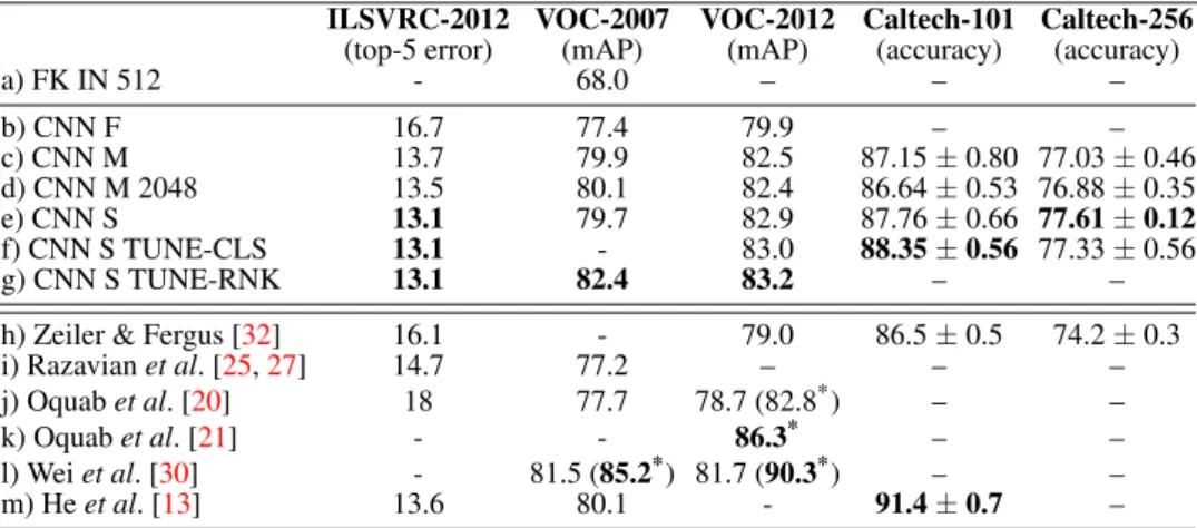
ILSVRC-2012 VOC-2007 VOC-2012 Caltech-101 Caltech-256 (top-5 error) (mAP) (mAP) (accuracy) (accuracy)

(a) FK IN 512 - 68.0 – – –

(b) CNN F 16.7 77.4 79.9 – –

(c) CNN M 13.7 79.9 82.5 87.15±0.80 77.03±0.46 (d) CNN M 2048 13.5 80.1 82.4 86.64±0.53 76.88±0.35 (e) CNN S 13.1 79.7 82.9 87.76±0.66 77.61±0.12 (f) CNN S TUNE-CLS 13.1 - 83.0 88.35±0.56 77.33±0.56

(g) CNN S TUNE-RNK 13.1 82.4 83.2 – –

(h) Zeiler & Fergus [32] 16.1 - 79.0 86.5±0.5 74.2±0.3 (i) Razavianet al. [25,27] 14.7 77.2 – – – (j) Oquabet al. [20] 18 77.7 78.7 (82.8*) – –

(k) Oquabet al. [21] - - 86.3* – –

(l) Weiet al. [30] - 81.5 (85.2*) 81.7 (90.3*) – – (m) Heet al. [13] 13.6 80.1 - 91.4±0.7 – Table 3: Comparison with the state of the art on ILSVRC2012, VOC2007, VOC2012, Caltech-101, and Caltech-256. Results marked with * were achieved using models pre-trained on the extendedILSVRC datasets (1512 classes in [20,21], 2000 classes in [30]). All other results were achieved using CNNs pre-trained on ILSVRC-2012 (1000 classes). in [26] but observed no improvement. Finally, we investigate pushing the parameters of the representation settingK=512 (rows[h]-[l]). Increasing the number of GMM centres in the model fromK=256 to 512 results in a further performance increase (e.g.[h]vs.[d]), but at the expense of higher-dimensional codes (125K dimensional).

Scenario 2: Deep representation (CNN) with pre-training. CNN-based methods consis-tently outperform the shallow encodings, even after the improvements discussed above, by a large∼10% mAP margin ([i]vs.[p]). Our small architecture CNN-F, which is similar to DeCAF [8], performs significantly better than the latter ([II]vs.[s]), validating our imple-mentation. Both medium CNN-M[m]and slow CNN-S[p]outperform the fast CNN-F[m] by a significant 2∼3% margin. Since the accuracy of CNN-S and CNN-M is nearly the same, we focus on the latter as it is simpler and marginally (∼25%) faster. Remarkably, these good networks work very well even with no augmentation[o]. Another advantage of CNNs compared to IFV is the small dimensionality of the output features, although IFV can be compressed to an extent. We explored retraining the CNNs such that the final layer was of a lower dimensionality, and reducing from 4096 to 2048 actually resulted in a marginal performance boost ([x]vs.[p]). What is surprising is that we can reduce the output dimen-sionality further to 1024D[y]and even 128D[z]with only a drop of∼2% for codes that are 32×smaller (∼650×smaller than our best performing IFV[i]). Note,`2_{-normalising the} features accounted for up to∼5% of their performance over VOC 2007; it should be applied before input to the SVM and after pooling the augmented descriptors (where applicable). Scenario 3: Deep representation (CNN) with pre-training and fine-tuning. We fine-tuned our CNN-S architecture on VOC-2007 using the ranking hinge loss, and achieved a significant improvement: 2.7% ([γ]vs.[n]). This demonstrates that in spite of the small

amount of VOC training data (5,011 images), fine-tuning is able to adjust the learnt deep representation to better suit the dataset in question.

Combinations. For the CNN-M 2048 representation[x], stacking deep and shallow repre-sentations to form a higher-dimensional descriptor makes little difference ([x]vs.[β]). For

the weaker CNN-F it results in a small boost of∼0.8% ([m]vs.[α]).

Comparison with the state of the art. In Table3we report our results on ILSVRC-2012, VOC-2007, VOC-2012, Caltech-101, and Caltech-256 datasets, and compare them to the

CHATFIELD ET AL.: RETURN OF THE DEVIL state of the art. First, we note that the ILSVRC error rates of our CNN-F, CNN-M, and CNN-S networks are better than those reported by [17], [32], and [27] for the related con-figurations. This validates our implementation, and the difference is likely to be due to the sampling of image crops from the uncropped image plane (instead of the centre). When using our CNN features on other datasets, the relative performance generally follows the same pattern as on ILSVRC, where the nets are trained – the CNN-F architecture exhibits the worst performance, with CNN-M and CNN-S performing considerably better.

Further fine-tuning of CNN-S on the VOC datasets turns out to be beneficial; on VOC-2012, using the ranking loss is marginally better than the classification loss ([g] vs. [f]), which can be explained by the ranking-based VOC evaluation criterion. Fine-tuning on Caltech-101 also yields a small improvement, but no gain is observed over Caltech-256.

Our CNN-S net is competitive with recent CNN-based approaches [13,20,21,25,30,32] and on a number of datasets (VOC-2007, VOC-2012, Caltech-101, Caltech-256) and sets the state of the art on VOC-2007 and VOC-2012 across methods pre-trained solely on ILSVRC-2012 dataset. While the CNN-based methods of [21, 30] achieve better performance on VOC (86.3% and 90.3% respectively), they were trained using extended ILSVRC datasets, enriched with additional categories semantically close to the ones in VOC. Additionally, [30] used a significantly more complex classification pipeline, driven by bounding box propos-als [5], pre-trained on ILSVRC-2013 detection dataset. Their best reported result on VOC-2012 (90.3%) was achieved by the late fusion with a complex hand-crafted method of [31]; without fusion, they get 84.2%. On Caltech-101, [13] achieves the state of the art using spa-tial pyramid pooling of conv5 layer features, while we used full7 layer features consistently across all datasets (for full7 features, they report 87.08%).

In addition to achieving performance comparable to the state of the art with a very simple approach (but powerful CNN-based features), with the modifications outlined in the paper (primarily the use of data augmentation similar to the CNN-based methods) we are able to improve the performance of shallow IFV to 68.02% (Table2,[i]).

Timings and dimensionality. One of our best-performing CNN representations CNN-M-2048[x]is∼42×more compact than the best performing IFV[i](84K vs. 2K) and CNN-M features are also∼50×faster to compute (∼120svs.∼2.4sper image with augmentation enabled, over a single CPU core). Non-augmented CNN-M features[o]take around 0.3sper image, compared to∼0.4sfor CNN-S features and∼0.13sfor CNN-F features.

5

Conclusion

In this paper we presented a rigorous empirical evaluation of CNN-based methods for im-age classification, along with a comparison with more traditional shallow feature encoding methods. We have demonstrated that the performance of shallow representations can be sig-nificantly improved by adopting data augmentation, typically used in deep learning. In spite of this improvement, deep architectures still outperform the shallow methods by a large mar-gin. We have shown that the performance of deep representations on the ILSVRC dataset is a good indicator of their performance on other datasets, and that fine-tuning can further im-prove on already very strong results achieved using the combination of deep representations and a linear SVM. Source code and CNN models to reproduce the experiments presented in the paper are available on the project website [4] in the hope that it would provide common ground for future comparisons, and good baselines for image representation research. Acknowledgements. This work was supported by the EPSRC and ERC grant VisRec no. 228180. We gratefully acknowledge the support of NVIDIA Corporation with the donation of the GPUs used for this research.

CHATFIELD ET AL.: RETURN OF THE DEVIL

References

[1] R. Arandjelovi´c and A. Zisserman. Three things everyone should know to improve object retrieval. InProc. CVPR, 2012.

[2] R. Arandjelovi´c and A. Zisserman. All about VLAD. InProc. CVPR, 2013.

[3] K. Chatfield, V. Lempitsky, A. Vedaldi, and A. Zisserman. The devil is in the details: an evaluation of recent feature encoding methods. InProc. BMVC., 2011.

[4] K. Chatfield, K. Simonyan, A. Vedaldi, and A. Zisserman. Return of the devil in the details: delving deep into convolutional nets webpage, 2014. URLhttp://www.

robots.ox.ac.uk/~vgg/research/deep_eval.

[5] M.-M. Cheng, Z. Zhang, W.-Y. Lin, and P. H. S. Torr. BING: Binarized normed gradi-ents for objectness estimation at 300fps. InProc. CVPR, 2014.

[6] G. Csurka, C. Bray, C. Dance, and L. Fan. Visual categorization with bags of keypoints. InWorkshop on Statistical Learning in Computer Vision, ECCV, pages 1–22, 2004.

[7] J. Deng, W. Dong, R. Socher, L.-J. Li, K. Li, and L. Fei-Fei. Imagenet: A large-scale hierarchical image database. InProc. CVPR, 2009.

[8] J. Donahue, Y. Jia, O. Vinyals, J. Hoffman, N. Zhang, E. Tzeng, and T. Darrell. De-caf: A deep convolutional activation feature for generic visual recognition. CoRR, abs/1310.1531, 2013.

[9] M. Everingham, L. Van Gool, C. K. I. Williams, J. Winn, and A. Zisserman. The PASCAL Visual Object Classes (VOC) challenge.IJCV, 88(2):303–338, 2010.

[10] L. Fei-Fei, R. Fergus, and P. Perona. Learning generative visual models from few training examples: An incremental bayesian approach tested on 101 object categories. InIEEE CVPR Workshop of Generative Model Based Vision, 2004.

[11] R. B. Girshick, J. Donahue, T. Darrell, and J. Malik. Rich feature hierarchies for accurate object detection and semantic segmentation. InProc. CVPR, 2014.

[12] G. Griffin, A. Holub, and P. Perona. Caltech-256 object category dataset. Technical Report 7694, California Institute of Technology, 2007. URLhttp://authors.

library.caltech.edu/7694.

[13] K. He, A. Zhang, S. Ren, and J. Sun. Spatial pyramid pooling in deep convolutional networks for visual recognition. InProc. ECCV, 2014.

[14] H. Jégou, M. Douze, and C. Schmid. On the burstiness of visual elements. InProc. CVPR, Jun 2009.

[15] H. Jégou, F. Perronnin, M. Douze, J. Sánchez, P. Pérez, and C. Schmid. Aggregating local images descriptors into compact codes.IEEE PAMI, 2012.

[16] Y. Jia. Caffe: An open source convolutional architecture for fast feature embedding.

CHATFIELD ET AL.: RETURN OF THE DEVIL [17] A. Krizhevsky, I. Sutskever, and G. E. Hinton. ImageNet classification with deep

con-volutional neural networks. InNIPS, pages 1106–1114, 2012.

[18] S. Lazebnik, C. Schmid, and J Ponce. Beyond Bags of Features: Spatial Pyramid Matching for Recognizing Natural Scene Categories. InProc. CVPR, 2006.

[19] Y. LeCun, B. Boser, J. S. Denker, D. Henderson, R. E. Howard, W. Hubbard, and L. D. Jackel. Backpropagation applied to handwritten zip code recognition. Neural Computation, 1(4):541–551, 1989.

[20] M. Oquab, L. Bottou, I. Laptev, and J. Sivic. Learning and Transferring Mid-Level Image Representations using Convolutional Neural Networks. InProc. CVPR, 2014.

[21] M. Oquab, L. Bottou, I. Laptev, and J. Sivic. Weakly supervised object recognition with convolutional neural networks. Technical Report HAL-01015140, INRIA, 2014.

[22] M. Paulin, J. Revaud, Z. Harchaoui, F. Perronnin, and C. Schmid. Transformation Pursuit for Image Classification. InProc. CVPR, 2014.

[23] F. Perronnin, J. Sánchez, and T. Mensink. Improving the Fisher kernel for large-scale image classification. InProc. ECCV, 2010.

[24] F. Perronnin, Z. Akata, Z. Harchaoui, and C. Schmid. Towards good practice in large-scale learning for image classification. InProc. CVPR, pages 3482–3489, 2012.

[25] A. Razavian, H. Azizpour, J. Sullivan, and S. Carlsson. CNN Features off-the-shelf: an Astounding Baseline for Recognition.CoRR, abs/1403.6382, 2014.

[26] J. Sánchez, F. Perronnin, and T. Emídio de Campos. Modeling the spatial layout of im-ages beyond spatial pyramids.Pattern Recognition Letters, 33(16):2216–2223, 2012.

[27] P. Sermanet, D. Eigen, X. Zhang, M. Mathieu, R. Fergus, and Y. LeCun. OverFeat: Integrated Recognition, Localization and Detection using Convolutional Networks. In Proc. ICLR, 2014.

[28] J. Sivic and A. Zisserman. Video Google: A text retrieval approach to object matching in videos. InProc. ICCV, volume 2, pages 1470–1477, 2003.

[29] A. Vedaldi and A. Zisserman. Efficient additive kernels via explicit feature maps.IEEE PAMI, 2011.

[30] Y. Wei, W. Xia, J. Huang, B. Ni, J. Dong, Y. Zhao, and S. Yan. CNN: Single-label to multi-label. CoRR, abs/1406.5726, 2014.

[31] S. Yan, J. Dong, Q. Chen, Z. Song, Y. Pan, W. Xia, H. Zhongyang, Y. Hua, and S. Shen. Generalized hierarchical matching for subcategory aware object classification. InThe PASCAL Visual Object Classes Challenge Workshop, 2012.

[32] M. D. Zeiler and R. Fergus. Visualizing and understanding convolutional networks. CoRR, abs/1311.2901, 2013.