Preprint, Jun 21, 2018
Parallel solution, adaptivity, computational
convergence, and open-source code of 2d and 3d
pressurized phase-field fracture problems
Timo Heister
∗Thomas Wick
†We present a scalable, parallel implementation of a solver for the solution of a phase-field model for quasi-static brittle fracture. The code is available as open source. Numerical solutions in 2d and 3d with adaptive mesh refinement show optimal scaling of the linear solver based on algebraic multigrid, and convergence of the phase-field model towards exact values of functionals of interests such as the crack opening displacement or the total crack volume. In contrast to uniform refinement, adaptive mesh refinement allows us to recover optimal convergence rates for the non-smooth solutions encountered in typical test problems. We also present numerical studies of the influence of the finite domain size on functional evaluations used to approximate the infinite domain.
Keywords: Phase-field fracture; parallel computing, scalability, influence of domain, deal.II
1 Introduction
In this work, we study the performance of the linear solver and the parallelization of our phase-field model for brittle fracture developed in [10] that allows 3d, adaptive solutions to more than 1024 cores and 100 million degrees of freedom. The original code was published onhttps://github.com/tjhei/ cracksand is based on the Finite Element library deal.II [1]. While solver aspects for a similar prolem have been discussed in [7], a scalable parallel implementation is novel.
We consider 2d and 3d benchmark problems in a pressurized fracture setting (Sneddon’s tests [12]). While seemingly simple, it is a challengening test problem (that is prototypical for most phase-field fracture configurations) for the following reasons: First, the underlying energy functional is non-convex. Second, the reference problem is defined on an infinite domain, so approximation with a finite domain introduces errors. Third, due to the smeared interface zone, accurate representations of the total crack volume (TCV) and crack opening displacement (COD) requires a small phase-field regularization parameter and a very high resolution mesh around the crack region.
∗
Mathematical Sciences, Clemson University, Clemson, SC 29634, USA, [email protected]
†
Institut f¨ur Angewandte Mathematik, Leibniz Universit¨at Hannover, Welfengarten 1, 30167 Hannover, Germany, [email protected]
2 Notation and equations
Let B ⊂ Rd, d = 2,3 the total domain wherein C ⊂ Rd−1 denotes the fracture and Ω ⊂ Rd is the unbroken domain. We assume homogeneous Dirichlet conditions on the outer boundary∂B. Using a phase-field approach, the lower-dimensional fracture C is approximated by ΩF ⊂B with the help of an elliptic (Ambrosio-Tortorelli) functional. For fracture formulations posed in a variational setting first proposed in [8], fracture regularizations using Ambrosio-Tortorelli functionals were developed in [4]. The unknown solution variables are vector-valued displacements u : B → Rd and a smoothed scalar-valued indicator phase-field function ϕ :B → [0,1]. Here ϕ = 0 denotes the crack region and ϕ = 1 characterizes the unbroken material. The intermediate values constitute a smooth transition zone dependent on a regularization parameterε. Adding a pressurep:B →Rthat acts on the fracture boundary was first rigorously modeled and mathematically analyzed in [11]. Next, the physics require a crack irreversibility condition (the crack can never heal), which is an inequality condition in time, i.e, ϕ≤ϕold, whereϕold denotes the previous time step solution. Consequently, modeling of fracture evolution problems leads to a variational inequality system, that is always, due to this constraint, quasi-stationary or time-dependent. Let V := H01(B), W := H1(B) and Win := {w ∈ H1(B)|w ≤ ϕold ≤ 1 a.e. onB} be the function spaces to state the variational formulation. In the following, we denote the L2 scalar product with (·,·). The Euler-Lagrange system for pressurized phase-field fracture reads [10, 11]:
Formulation 1. Let p ∈ L∞(B) be given. For the loading steps n = 1,2,3, . . .: Find vector-valued displacements and a scalar-valued phase-field variable {u, ϕ}:={un, ϕn} ∈ {u
D+V} ×W such that
(1−κ) ˜ϕ2+κσ(u), e(w)
+ (ϕ2p,div w) = 0, (1)
(1−κ)(ϕ σ(u) :e(u), ψ−ϕ) + 2(ϕ pdivu, ψ−ϕ) +Gc
−1 ε(1−ϕ, ψ−ϕ) +ε(∇ϕ,∇(ψ−ϕ)) ≥0, (2)
for all w ∈ V and ψ ∈ Win ∩L∞(B). Here, Gc is the critical energy release rate, and we use the well-known law for the linear stress-strain relationship σ:=σ(u) = 2µse(u) +λstre(u)I, whereµs>0 and λs>0 denote the Lam´e coefficients, e(u) = 21(∇u+∇uT) is the linearized strain tensor and I is the identity matrix, κ >0. Finally, ϕ˜ is a linear extrapolation in time developed in [10] in order to convexify the above problem.
3 Solution algorithms and parallel framework
To solve Formulation 1, we employ a semi-smooth Newton method that was developed for phase-field fracture in [10] and combines two Newton methods: solving the nonlinear problem and treating the irreversibility constraint. The spatial discretization is based on a Galerkin finite element scheme, introducing H1 conforming discrete spaces Vh ⊂ V and Wh ⊂ W consisting of bilinear/trilinear functions Qc1 on quadrilaterals / hexahedra, respectively. The discretization parameter is denoted by h. The code is fully parallelized using MPI by building on the deal.II finite element library [1]. The adaptive meshes are handled by p4est [5] and the linear algebra is built on Trilinos [9]. This software framework is discussed in [2].
From our original work [10], we extended the active set strategy with a method to detect and constrain alternating active set indices to avoid cycles of the method similar to [6]. Additionally, we extended our refinement strategy from not only refining in the crack region to enforce ε= 2h to also include a gradient jump estimator for the displacements. This is required to achieve rigorous computational convergence of the benchmark problem discussed here.
3.1 Linear iterative solution
The linear systems arising at each Newton step are solved iteratively using a GMRES scheme with a block diagonal preconditioner P−1:
Muu 0 Mϕu Mϕϕ δu δϕ = Fu Fϕ with P−1= ˜ Muu−1 0 0 M˜ϕϕ−1 .
Using the basis {ψi|i = 1, . . . , N} in Vh ×Wh with ψi = (χui,0)T, i = 1, . . . , Nu and ψNu+i = (0, χϕi)T, i= 1, . . . , Nϕ and N =Nu+Nϕ, we have specifically the entries:
(Muu)i,j =
(1−κ) ˜ϕ2+κσ(χuj), e(χui)
+ (σ(χuj), e(χui)), (Mϕu)i,j = 2(1−κ)(ϕ σ(χuj) :e(u), χ
ϕ i)−2(α−1)p(ϕdiv(χ u j), χ ϕ i), (Mϕϕ)i,j = (1−κ)(σ(u) :e(u)χϕj, χϕi)−2(α−1)p(div(u)χϕj, χϕi) +Gc
1 ε(χ ϕ j, χ ϕ i) +ε(∇χ ϕ j,∇χ ϕ i) . The block Muϕ is zero due ˜ϕin Equation (1).
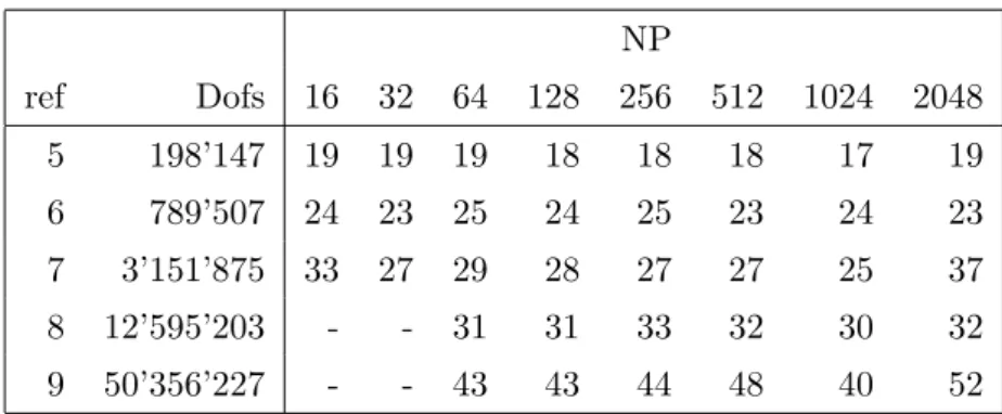
We assume the existence of spectrally equivalent approximations ˜Muu−1 and ˜Mϕϕ−1, which correspond to linear elasticity and a mixture of a Laplacian and mass matrix, respectively. The eigenvalues are given by the generalized eigenvalues of the systems ˜Mkk = λMkk (k =u, ϕ). We are approximating the blocks using a single V-cycle of algebraic multigrid (by Trilinos ML, [9]). Assuming the multigrid gives approximations independent of the mesh size h, the whole solver scheme is nearly optimal and independent of the number of processors and mesh size, as can be seen in Table 1.
NP ref Dofs 16 32 64 128 256 512 1024 2048 5 198’147 19 19 19 18 18 18 17 19 6 789’507 24 23 25 24 25 23 24 23 7 3’151’875 33 27 29 28 27 27 25 37 8 12’595’203 - - 31 31 33 32 30 32 9 50’356’227 - - 43 43 44 48 40 52
Table 1: Number of GMRES iterations of a single Newton step for the Sneddon 2d test with global refinement. Iterations are nearly independent of problem size (h) and number of processors N P. The relative residual is 1e-8.
Remark 1. The parallelized linear solution of phase-field fracture was already implemented in [10] for 2d problems, but a computational analysis of the performance and the extension to 3d settings was missing up to now in the existing literature.
4 Numerical tests: Sneddon 2d and 3d
We perform numerical tests in 2d and 3d. The benchmarks are based on the theoretical calculations of [12][Section 2.4 and Section 3.3]. A (constant) pressure p= 10−3P a causes the fracture to change its width but not the length to form a penny-shaped crack. The initial crack of length l0 = 1.0
is described with the help of the phase-field function ϕ. The domains are varied as (−K, K)d, d = 2,3, K = 5,10,20,40 to approximate the infinite domain of the benchmark. We choose Gc = 1, Youngs’ modulus as E = 1 and Poisson’s ratio is ν = 0.2. The regularization parameters are chosen asε= 2h andκ= 10−12h. For more details of our computational configuration we refer the reader to [10][Section 5.3] (2d) and [13][Section 5.4] (3d).
We study the total crack volume (TCV) with analytical solutions from [12], respectively:
T CVh,= Z Ω u· ∇φdx, T CV2d= Z x 2uy(x)dx= 2πpl2 0(1−ν2) E , T CV3d= Z x Z y 2uz(x, y)dxdy = 16pl3 0(1−ν2) 3E (3)
wherel0 = 1.0,E= 1.0,p= 1e−3,ν = 0.2. We note that the crack opening displacement (COD) is
computed by un(v) = cpl0(1−ν2) E s 1− ρ l0 2
, with the radius ρ=kxkl2, x∈Rd
withn=y, v=x, c= 2 in 2dandn=z, v= (x, y), c= 4/π in 3d.
4.1 Convergence of total crack volume (TCV) in 2d
The first set of computations computes the error of the TCV in 2d for fixed values ofεwhile adaptively refining the solutions. Convergence for h → 0 and ε → 0 are clearly visible; see Fig. 1, left. This computation demonstrates: First, the phase-field regularization is a valid and convergent approxima-tion of the fracture problem. Second, our approach for adaptive refinement is effective and the choice of ε= 2h combined with adaptivity is a valid implementation strategy, that gives accurate solutions with a few number of unknowns.
102 103 104 105 106 # DoFs 10−1 100 101 relative crack volume error eps=1 eps=1/2 eps=1/4 eps=1/8 eps=1/16 eps=1/32 eps=2h 103 104 105 106 # DoFs 0.006 0.008 0.01 total crack volume reference 10x10 20x20 40x40 80x80
Figure 1: Left (Section 4.1): The convergence ofε on the 40x40 domain is computationally analyzed. Here we observe linear convergence in epsilon. Right (Section 4.2): dependence of functional value evaluations on the domain size.
4.2 Influence of finite domain size in 2d
The benchmark problem is stated for an infinite domain, so convergence is only obtained until this part of the error becomes dominant as can be seen in Fig. 1 (right). A larger size of the domain would raise the cost of the discretization immensly without adaptive mesh refinement, while we obtain more accurate solutions on a larger domain with about 105 unknowns and our refinement strategy. The extrapolated value of the TCV compared to the exact value of 6.0319E-03 has an error of 5.6%, 1.5%, 0.5%, and 0.1% for the domain size of 10x10, 20x20, 40x40, and 80x80, respectively.
4.3 Convergence of the 3d benchmark
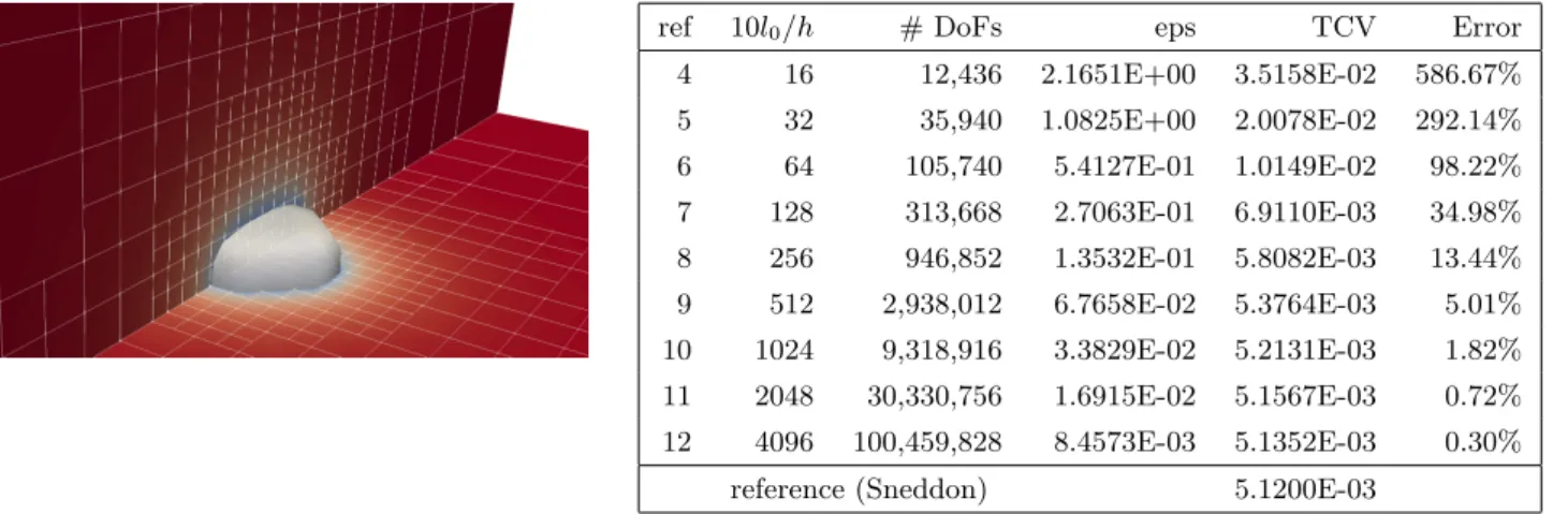
We now concentrate on the convergence of the TCV error for the 3d version of the same benchmark problem. Even with adaptive refinement, an accurate solution requires in the order of 100 million DoFs and substantial computing power (here run on 1 024 cores); see Figure 2. On the one hand, this is a well-known challenge for smeared interface approaches. On the other hand, 3d compu-tations for moving interface problems are still a challenge for ‘exact’ interface represencompu-tations such as extended/generalized finite elements, cut cell methods, etc.. Therefore, these results show that phase-field approaches can give comparable results to other numerical methods.
ref 10l0/h # DoFs eps TCV Error
4 16 12,436 2.1651E+00 3.5158E-02 586.67% 5 32 35,940 1.0825E+00 2.0078E-02 292.14% 6 64 105,740 5.4127E-01 1.0149E-02 98.22% 7 128 313,668 2.7063E-01 6.9110E-03 34.98% 8 256 946,852 1.3532E-01 5.8082E-03 13.44% 9 512 2,938,012 6.7658E-02 5.3764E-03 5.01% 10 1024 9,318,916 3.3829E-02 5.2131E-03 1.82% 11 2048 30,330,756 1.6915E-02 5.1567E-03 0.72% 12 4096 100,459,828 8.4573E-03 5.1352E-03 0.30%
reference (Sneddon) 5.1200E-03
Figure 2: Section 4.3: Sneddon 3d adaptive convergence for a 10x10x10 domain,l0= 1, usingε= 2h.
Left: solution with mesh and isosurface forϕ= 0.3. Right: convergence table.
4.4 Adaptive convergence of crack opening displacement (COD)
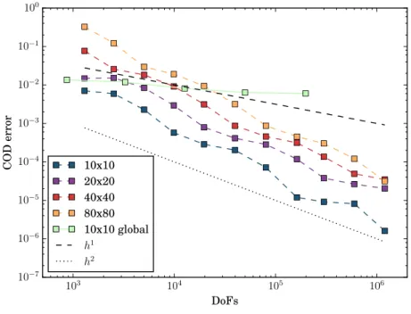
Finally, we study the crack opening displacement (COD) in 2d to compare adaptive vs. global re-finement. For each domain size, the reference value is obtained using Richardson extrapolation of the numerical solution. As the solution is discontinuous, we see suboptimal convergence of the solution using global refinement, while we recover optimal rates using our adaptive scheme; see Figure 3.
Our results suggest a convergent method and lead us to expect an error estimate of the kind (similar to [14])
kuh,ε−urefk ≤ kuh,ε−uref,εk+kuref,ε−urefk ≤C1inf
where the error of the discrete solution uh,ε to the exact solution uref is given by the sum of best-approximation error of the finite element method and an error term (i.e., a model error) introduced by the εregularization converging linearly in ε.
103 104 105 106 DoFs 10−7 10−6 10−5 10−4 10−3 10−2 10−1 100 COD error 10x10 20x20 40x40 80x80 10x10 global h1 h2
Figure 3: Section 4.4: Sneddon 2d error convergence to extrapolated COD values for a fixed domain size. We recover quadratic convergence inh using our adaptive refinement strategy. Errors are increasing for a fixed number of unknowns for a larger domain size, as the crack is resolved with fewer cells.
Acknowledgements
This work is supported by the German Priority Programme 1748 (DFG SPP 1748) Reliable Simulation Techniques in Solid Mechanics. Development of Non-standard Discretization Methods, Mechanical and Mathematical Analysis. Timo Heister was partially supported by the Computational Infrastructure in Geodynamics initiative (CIG), through the NSF under Award EAR-0949446 and The University of California Davis, by the NSF Award DMS-1522191, and by Technical Data Analysis, Inc through US Navy SBIR N16A-T003. Clemson University is acknowledged for generous allotment of compute time on Palmetto cluster.
References
[1] D. Arndt, W. Bangerth, D. Davydov, T. Heister, L. Heltai, M. Kronbichler, M. Maier, J.-P. Pelteret, B. Turcksin, and D. Wells. J. Numer. Math.,25, 137–146 (2017).
[2] W. Bangerth, C. Burstedde, T. Heister, and M. Kronbichler. ACM Trans. Math. Softw., 38, 14/1–28 (2011).
[3] W. Bangerth, R. Hartmann, and G. Kanschat, ACM Trans. Math. Softw.33, 24/1–24/27 (2007). [4] B. Bourdin, G.A. Francfort, and J.-J. Marigo, J. Mech. Phys. Solids 48, 797–826 (2000).
[5] C. Burstedde, L. C. Wilcox, and O. Ghattas, SIAM J. Sci. Comput.,33, 1103–1133 (2011). [6] F. E. Curtis, Z. Han, D. P. Robinson, Computational Optimization and Applications,60, 311-341
(2015).
[7] P. E. Farrell and C. Maurini, Int. J. Numer. Meth. Engrg.,109, 648–667 (2017). [8] G.A. Francfort and J.-J. Marigo, J. Mech. Phys. Solids 46, 1319–1342 (1998).
[9] M. Heroux, R. Bartlett, V. H. R. Hoekstra, J. Hu, T. Kolda, R. Lehoucq, K. Long, R. Pawlowski, E. Phipps, A. Salinger, H. Thornquist, R. Tuminaro, J. Willenbring, and A. Williams. An Overview of Trilinos, Technical Report SAND2003-2927 (2003).
[10] T. Heister, M. F. Wheeler, and T. Wick, Comp. Meth. Appl. Mech. Engrg.290, 466 – 495 (2015). [11] A. Mikeli´c, M. Wheeler, and T. Wick, ICES Report14-18(2014).
[12] I. N. Sneddon and M. Lowengrub, Crack problems in the classical theory of elasticity, SIAM series in Applied Mathematics. John Wiley and Sons, Philadelphia, 1969.
[13] M. F. Wheeler, T. Wick, W. Wollner, Comp. Meth. Appl. Mech. Engrg. 271, 69–85 (2014). [14] T. Wick, Comp. Mech., 57(6), 1017–1035 (2016).