IS
THERE
AN
ALTERNATIVE
STRATEGY
FOR
REDUCING
PUBLIC
DEBT
BY
2032?
Christophe Blota, Marion Cocharda, Jérôme Creelb, Bruno Ducoudréa, Danielle Schweisgutha and Xavier Timbeaua
a. OFCE (Centre de recherche en économie de Sciences Po) b. OFCE and ESCP Europe
First draft
1. Introduction
Expansionary fiscal policies undertaken in 2009, when the world economy was strongly hit by the worst financial crisis since the Great Depression, have been short-lived. EMU countries have indeed clearly engaged a consolidation of fiscal policies since 2011. The objectives are twofold. On the short run, governments aim at bringing back the deficit ratio to 3 % of GDP, as recommended by the Stability and Growth Pact. On the long run, in accordance with the new fiscal rules, the objective is to reach a debt ratio of a least 60 % of GDP by 2032. For the advocates of such a frontloaded strategy, consolidation is needed to restore credibility of fiscal policies. The sovereign debt crisis has indeed urged national governments to ensure the issue of the sustainability of public finances. The rise of financial market pressures, the lack of a "true" central bank, and the absence of mutualisation between member states explained this choice. Yet as this paper shows, this choice is not a valid one.
This strategy is unambiguously costly. It puts a drag on demand and triggers a rise in unemployment. The question is then, how large are these costs and is there an alternative strategy? The aim of the paper is precisely to deal with these issues. It considers explicitly that the euro area is facing a tradeoff between unemployment and public debt, both of which are interlinked. Up to now, the Eurozone has given the priority to the reduction of public debt. But as it has recently been highlighted by Holland and Portes (2012), this
strategy is self-defeating. The Eurozone entered a new recession, the reduction path of public deficits is disappointing regarding the strong negative fiscal stance and the liquidity crisis1 on the debt markets eased only after the announcement by the ECB that it might
intervene under certain conditions. This paper does not only confirm the failure of the strategy of a frontloaded consolidation. It discusses alternative scenarios built from a simulations based on a reduced-form model. More precisely, we suggest keeping the target of a debt ratio of 60 % by 2032 but spreading or delaying and spreading consolidation would improve growth. So that, for most countries, long-term sustainability of public finances is maintained while in the short run, growth is higher.
The main reason of this failure is that austerity policies have been implemented in countries which are already facing a highly degraded economic situation in which fiscal multipliers are high. A growing literature on fiscal multipliers have indeed emphasized that fiscal multipliers are higher during recessions than in normal times2. In such a case, attempting to reduce debt by fiscal consolidation brings more debt and more unemployment. Spain is the perfect illustration of this very frustrating dynamics. Consolidation should be postponed until fiscal multipliers are smaller and unemployment lower.
Besides, we stress that existing treaties and the fiscal compact allow for a more relaxed path for fiscal consolidation. What is considered as valid by the treaties should be the reference for fiscal consolidation. Such a plan should be based on a pragmatic view on what is suitable for debt sustainability over the next 20 years.
To judge the interactions between debt and unemployment reduction, we develop a simple reduced-form model representing eleven countries of the euro area (Austria, Belgium, Finland, France, Germany, Greece, Ireland, Italy, the Netherlands, Portugal and Spain). This model aims to be sufficiently detailed to explicitly link all macro elements of debt sustainability and output dynamics. Then, as a strong debate still exists about the value of multipliers and about the evaluation of today's output gaps, and also because there is of course irreducible uncertainty about future growth, we have chosen to parameterize the model in such a way that we can conduct a full sensitivity analysis. Finally, we had in mind that the model would have to address the search for the optimal fiscal stance, defined as a better fiscal consolidation under some strong constraints.
The rest of the paper is organized as follows. Beforehand, we draw on the EU fiscal framework to assess the stringency of EU fiscal rules and explore the scope for an alternative strategy to ensure fiscal sustainability in due respect of EU regulations and treaties. The model is described in a second section. The third section shows that the actual path of consolidation is ill-designed. Finally, the fourth section present alternative strategies.
1
See De Grauwe and Yi (2013) for analysis of the failure of austerity to dampen panic on the financial markets.
2
See Almunia, Bénétrix, Eichengreen, O’Rourke and Rua (2010) for an arguement based on the situation during the
2. Margins for manoeuvre within the actual EU fiscal framework
There are currently five fiscal rules which must be fulfilled by EU Member States. Except for one fiscal rule exclusively related to the Fiscal Compact—the new medium-term fiscal objective, see fifth fiscal rule below—all EU fiscal rules have been in force since at least November 2011.
First, the cornerstone of European fiscal rules remains the public deficit to GDP limit at 3%. Deficits above this threshold can be labelled "excessive deficits", setting in train an excessive deficit procedure.
Second, the public-debt-to-GDP ratio must be limited to 60% of GDP or it must be decreasing towards this level.
The first and second fiscal rules are embedded in the Stability and Growth Pact originally introduced in 20053. They were confirmed by the revised Stability and Growth Pact adopted in November 2011 under Council Regulations 1173/2011, 1175/2011 and 1177/2011.
Third, if the public-debt ratio is above the threshold limit, the ratio will be considered to diminish at a sufficient pace if the difference between actual debt and the 60%-of-GDP limit has been decreasing during the three preceding years at an average yearly rate of 1/20th of
the difference. This 1/20th debt rule is incorporated in the revised Stability and Growth Pact
adopted in November 2011 under Council Regulation 1177/2011, article 2, par. 1bis. It has also been included in the Fiscal Compact, article 4, of the Treaty on Stability, Coordination and Governance in the EMU of March 2012.
Fourth, if a Member State is under an excessive deficit procedure, Council Regulation 1177/2011, article 3, states that: "in its recommendation, the Council shall request that the Member State achieve annual budgetary targets which, on the basis of the forecast underpinning the recommendation, are consistent with a minimum annual improvement of at least 0.5 % of GDP as a benchmark, in its cyclically adjusted balance net of one-off and temporary measures, in order to ensure the correction of the excessive deficit within the deadline set in the recommendation". In its article 5, Regulation 1175/2011 restates the same benchmark of a yearly improvement of 0.5% of GDP of the cyclically-adjusted deficit to reach the medium-term fiscal objective of a balanced-budget expressed in structural terms.
Fifth, the medium-term fiscal objective was made more precise in the Fiscal Compact, article 3. It states that general government budgets shall be balanced or in surplus, a criterion that "shall be deemed to be respected if the annual structural balance of the general government is at its country-specific medium-term objective, as defined in the
3The first rule has been the cornerstone of European fiscal rules since 1997 and the first version of the Stability and Growth Pact, whereas the second rule was only a convergence criterion between 1997 and 2005, before it was introduced in the first reformed version of the SGP. Legally speaking, the debt-rule was not a binding constraint on Euro area members states between 1999 (creation of the euro) and 2005.
revised Stability and Growth Pact, with a lower limit of a structural deficit of 0.5 % of the gross domestic product at market prices".
Some of the above-mentioned rules are conditional on exceptional circumstances. Such has always been the case for the first rule. However the strictness of exceptional circumstances has largely changed over the years. Between 1999 and 2005, exceptional circumstances meant a recession: a yearly real GDP growth rate of at least -2% permitted automatically delayed austerity to converge towards the 3%-of-GDP limit for the public deficit and balanced budget in the mid-run. A yearly real GDP growth rate of at least -0.75% permitted delayed austerity provided a majority of MS approved these exceptional circumstances. In 2005, the scope of exceptional circumstances was widened to encompass the implementation of structural reforms that were elaborated to cope with the Lisbon agenda strategy, and the implementation of public investment. Moreover, an unexpected economic slowdown could be considered as exceptional circumstances.
The 2011 body of legislation—the 6-pack—recalls the reform of the 1997 version of the SGP. It opens up a scope to use pension reforms as authorizing a public finances' gap vis-à-vis the convergence path towards the medium-run deficit objective (article 5, regulation 1175/2011). The fiscal compact introduced the following (complementary) definition of exceptional circumstances: "an unusual event outside the control of the (MS) which has a major impact on the financial position of the general government or periods of severe economic downturn as set out in the revised SGP, provided that the temporary deviation (…) does not endanger fiscal sustainability in the medium-term" (article 3, (b)). The definition of an "unusual event" remains unclear.
Finally, the first and fifth EU fiscal rules are conditional on exceptional circumstances. Drawing on these circumstances and on the fourth rule of a yearly improvement of 0.5% of GDP of the cyclically-adjusted deficit, it is possible to show that EU fiscal rules give fiscal leeway under current economic circumstances.
As a conclusion, the implementation of structural reforms should not be viewed as the only justification for softening the stance on fiscal austerity: severe economic downturn is also included as an exceptional circumstance to postpone fiscal efforts, and achievements of cyclically-adjusted annual improvements of public finances above a threshold of 0.5% of GDP are not legally required.
The EU does not have to change its position in order to soften the fiscal stances of Euro area countries facing excessive deficits. Notwithstanding a possible change in this position in the future, there are already ample margins for manoeuvre in the short run to escape "self-defeating austerity" under the present legislation.
The following modelling exercise shows just how important it is that these margins for manoeuvre are fully exploited by EU Member States.
3. Description of the model
The model is a macroeconomic model that combines structural and reduced-form non linear equations. Since one of its goals is to model numerous euro area countries, we use simple reduced-form equations to model supply and demand complex mechanisms that can be heterogeneous across countries. Hence the model is not the product of an optimal behaviour: there are multiple competing ways to obtain them though no consensus has emerged so far on best modelling strategies4. Moreover, Dynamic Standard General
Equilibrium (DSGE) models proved to perform poorly during the crisis5, underestimating the
deepness of the crisis. These models also do not allow to model nonlinearities such as variable fiscal multipliers over the business cycle, since these models are linearised around a single point. We then prefer simplicity in modelling, as it allows us to simply calibrate the impact of specific effects of fiscal policy on output gap and potential GDP.
Some key featuresof the model follow:
The model allows for an explicit representation of the main countries of the euro area: Austria, Belgium, Finland, France, Germany, Greece, Ireland, Italy, Netherlands, Portugal and Spain. An aggregated euro area is also computed in order to deal with global analysis and monetary policy.
On the demand side, an open economy aggregate demand function is modelled which embodies fiscal and monetary policy, external demand (a channel for intra EU interdependencies) as well as exogenous shocks on the output gap (the gap between actual and potential GDP). This equation also takes into account possible long run effects of macroeconomic policies such as long term fiscal policy, threshold effects or hysteresis on potential output. The parameterization allows simulating standard hypothesis as well as alternatives, checking to show the dependence of results on different sets of hypotheses. Furthermore, the size of fiscal multipliers is allowed to on the stage of the business cycle, and on the level of public debt. The effectiveness of monetary policy is allowed to differ when monetary policy hits zero lower bound.
External demand is modelled using a bilateral trade matrix representing interdependencies between countries. That trade matrix will also be used as a basis for imbalances analysis.
We model prices by a generalized Phillips curve relating current and expected inflation to economic activity, imported inflation and other exogenous shocks. Expectations can be modelled as adaptive (backward-looking) or rational (forward-looking).
4 See for example Wieland et al (2012) for a comparison of fiscal policy effects on output gap for a large set of DSGE models. These models make different assumptions on the share of liquidity constrained households for example, a point that is crucial to assess the fiscal multiplier.
5
A Taylor rule sums up monetary policy. Fiscal policy can be modelled with some kind of rule adjusting spending or taxes to debt or unemployment goals for example. Such rules can be unplugged to deal with optimal or alternate policy scenarios.
Fiscal policy, that is to say the public balance, separates interest payments, cyclically-adjusted balance and cyclical components, in order to properly assess the fiscal stance, i.e. the part of fiscal policy which is under the direct control (discretion) of current governments. We then deduce public debt projections for euro area countries. This module will help to assess fiscal sustainability issues, as it incorporates issues related to the impact of the market interest rate (government-bond yield).
Aggregate demand and supply
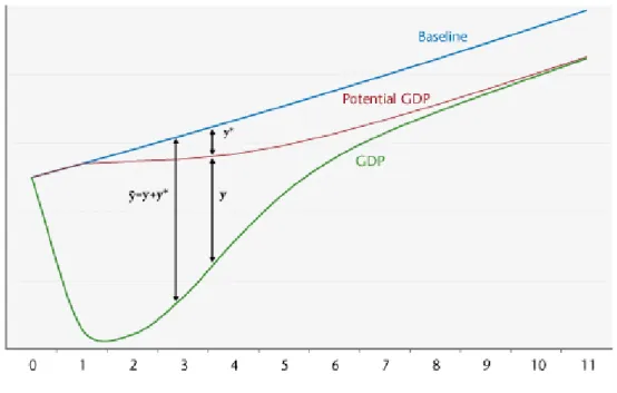
First, in the model GDP is written as a gap between the actual level of GDP and a baseline trajectory determined by a constant potential growth. However, we distinguish this baseline from the potential GDP, which can differ from the baseline due to possible hysteresis effects of recession or fiscal policy on potential GDP (see Figure 1 below). As a result, we model three gaps for GDP:
is the gap between log of real GDP of country c, and its baseline trajectory which is exogenous.
∗ is the gap between log of potential GDP ∗ of country c and the baseline .
Dropping country subscripts, the resulting output gap follows:
(1) ∗
is driven by aggregate demand in the short run:
(2) . .
is the effective fiscal impulse, which sums up the fiscal policy effects on aggregate demand (see the following sections). is the long term real interest rate on private bonds and is its long run equilibrium value. . sums up the effect of monetary policy on aggregate demand via its impact on financial markets and expectations of future inflation. . sums up the impact of addressed demand by trade partners. Combining equations (1) and (2) then gives:
The dynamics of equation (3) is simply given by the following error correction equation6:
(4) . ∗ . .
. . .
is the cumulated sum of past and current ex ante effective fiscal impulses, and its variation gives the short run impact of fiscal policy on . This impact depends on the endogenous fiscal multiplier which is discussed later. is an exogenous shock on aggregate demand.
We also restrict dynamics of equation (4). The idea is the following: when output gap is wide open, the error correction model implies a growth rate that can be very large, whereas recovery growth can be bound. Hence we limit the variation of before effects of monetary policy, fiscal policy and external trade. It gives:
. ∗ . ; 0.025
. . . .
.
It implies a maximum growth rate equal to the potential growth rate plus 2.5%.
Second, the gap between potential GDP and the baseline depends on a hysteresis effect, a long run impact of fiscal policy and a negative public debt effect:
(5) ∗ ∗ .
∝ . ∗
is an hysteresis parameter, ∝ assesses the long run impact of fiscal policy on
potential GDP (we discuss this point in the Fiscal policy section hereafter), stands for a Barro-Laffer effect, ∗ is a public debt target and an exogenous shock on aggregate
supply.
The Barro-Laffer effect mixes the requirement to increase private savings to match lower public savings – the Barro-Ricardo effect – with the requirement to levy higher taxes in the future to repay debt and interests. The latter is associated with disincentives to produce according to the Laffer effect. Lower private savings and higher disincentives to produce would drag potential output7.
6 stands for time subscript and ∆ .
7 There may also be some non-linearities as regards the relationship between public debt and real economic growth. Some argue (Reinhart and Rogoff, 2010, Ceccheti et al., 2011) that above a certain threshold of public debt, the latter reduces economic growth, though Panizza and Presbitero (2012) tend to reverse the causality. Panizza and Presbitero (2012) also highlight that high debt country may fear a loss of confidence from their creditors (the market)
Figure 1. Example: GDP path and potential GDP path with hysteresis
Source: iAGS model, OFCE.
Level and Growth rates of GDP
The growth rate of the baseline for real GDP is set exogenously: (6)
The growth rate of potential GDP is equal to the baseline one if there is no long run impact of fiscal policy, no hysteresis and no Barro-Laffer effect:
(7) ∗ ∗
The growth rate of real GDP is given by that of potential GDP and the output gap, the growth rate of nominal GDP takes into account the inflation rate, and the level of nominal GDP follows:
(8) ∗
(9)
(10) 1
and may decide upon a fiscal contraction that drags economic growth, hence a negative causality between high debt and economic growth.
Public finances
is the fiscal surplus in % of nominal GDP. We decompose it between a structural primary surplus and a cyclical surplus , minus government interest payments on public debt :
(11)
(12) . ∗
(13) .
(14) . 1
(15) 1⁄ . 1 1⁄ .
(16) ⁄ 1
The structural primary surplus evolves according to the fiscal impulse and changes in taxes due to variations in the gap between potential production and the baseline (eq. (12)). This latter point means that a permanent downward shift of potential production relative to the baseline would entail a permanent fall in taxes, then a permanent fall in the structural primary surplus.
The cyclical surplus depends on , the overall sensitivity of revenues and expenditures to the business cycle (eq. (13)). Interest payments on debt (in % of GDP) depend on the stock of debt times its average interest rate, and deflated by the nominal GDP growth rate (eq. (14)).
The average interest rate on debt evolves according to the long term nominal interest rate on newly issued public bonds. stands for the average maturity of public debt, and is assumed to be constant. 1 then gives the share of debt refinanced every year (eq. (15)).
Public debt (in % of nominal GDP) evolves according to past debt deflated by the nominal growth rate of GDP, minus the fiscal surplus, augmented with an exogenous stock-flow adjustment variable (eq. (16)).
Fiscal policy
The impact of fiscal policy is modelled according to the state of the economy. This modelling strategy has been growing recently in the literature (Parker, 2011), after empirical papers show that the fiscal multiplier differs according to the position of the economy in the cycle. For example, using regime-switching models, Auerbach and Gorodnichenko (2010) estimate effects of tax and spending policies that can vary over the business cycle. They
find large differences in the size of fiscal multipliers in recessions and expansions: fiscal policy is considerably more effective in recessions than in expansions. Assuming that the economy can endogenously switch between regimes, they find that historical multipliers can vary between 0 and 0.5 during expansions and between 1 and 1.5 during recessions8. The fiscal multiplier is modelled as follows:
If then
if then
if then
if then ⁄ ∗
if then ⁄ ∗
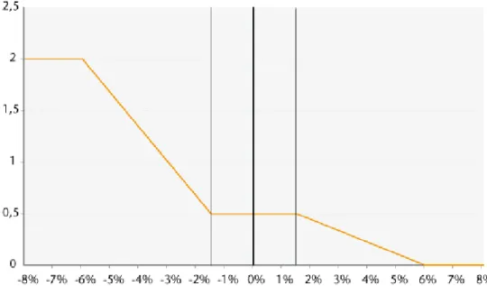
The value of the multiplier is maximal in very bad times, whereas it is minimal in very good times (see Figure 1).
Figure 2. Example of the value of the multiplier according to the output gap
Note: 2, 0.5, 0, 6%, 1.5%, 1.5%, and 6%. Values are taken as illustrative and may vary across countries.
Source: OFCE.
Fiscal policy, via the fiscal impulse (in % of GDP), drives the structural primary surplus. The fiscal impulse sums up discretionary decisions on government spending and taxes. We
8 See Baum and Koester (2011) for empirical estimates for Germany and Creel et al. (2011) for France; see Michaillat (2012) for a theoretical approach.
then compute an effective fiscal impulse: It is the ex ante9 cumulative real effect of current and past fiscal impulses at time t. Thus, with . . the fiscal multiplier at time t of a fiscal impulse that occurred years ago, we can write:
(17) . . . .
. . . .
(18) .
Equation (17) ensures that the impact of a fiscal impulse depends on the fiscal multiplier that prevailed at the date the fiscal impulse occurred. We retain seven lags to account for the possibility of long lasting effects of fiscal impulses. We also assume that can take into account long run effect of fiscal policy. It is the case if ∝ ∑ 0, since in that
case is not necessarily null in the long run10. The long run impact of a sequence of fiscal impulses is then computed using the accumulation of fiscal impulses times the multiplier (eq ((18)), and the long run impact on potential GDP is ∝.Σ .
External trade
We model external trade using trade matrix between euro area countries. Imports of each country grow up relative to the baseline imports when output rises. The strength of the increase depends on sensitivity of imports to the output gap (eq. (19)).
Imports of one country divide into exports of the other countries. Each country faces an addressed demand composed of imports of trade partners. The addressed demand to country c is the sum of imports of other j countries times the share of imports of country j
coming from country c (eq. (20)).
(19) .
(20) ∑ , ,
Monetary policy and financial markets
We use a Taylor rule to describe monetary policy (Taylor, 1993). The short term interest rate varies according to the gap between euro area inflation and the ECB target ∗ on
the one hand, and with the euro area output gap on the other hand (eq. (21)). ∗ is the
9 It is an ex ante multiplier in the sense that it does not take into account monetary policy effects and feedback effects of external trade on GDP following a fiscal impulse.
10 In that case we introduce a correction term in equation (4) to avoid counting twice the long run impact of fiscal policy on via ∗ and .
ECB long run target, hence the real equilibrium interest rate. We also account for a zero lower bound. The rate set by ECB is then the max of these two rates (eq. (22)).
According to the expectations theory, the long term interest rate for German public bonds is set equal to the expected sum of future short term interest rates (eq. (23); see Shiller, 1979).
The long term public rate for Germany is considered risk free, and long term public rates of other countries include a risk premium that is set exogenously (eq. (24)). We also temporarily set exogenously the long rate for countries that entered the EFSF to account for a lower interest rate on debt refinancing. Finally, for each country the long term interest rate on private bonds is equal to the public one plus a risk premium that is set exogenously (eq. (25)). The long term real interest rate on private bonds is then equal to the private nominal long term rate minus long run expected inflation (eq. (26)).
(21) ∗ . ∗ .
(22) ;
(23) . 1 .
(24) (25)
(26) ,
Prices
We model the growth rate of GDP price as a new Keynesian hybrid Phillips curve (NKHPC hereafter). Inflation depends on past inflation, expected inflation one period ahead, output gap, and the variation of overseas inflation weighted by the share of imports coming from country c (eq. (27)).
Different possible formations of inflation expectations can be introduced. Expectations can be rational as in a standard NKHPC equation , or they can be adaptive (eq. (28)). In this last case, we assume that inflation is expected to converge to the ECB target at a speed depending on the value of the parameter.
For financial markets, long run expected inflation is modelled as the discounted sum of future inflation rates (eq. (29)), in the same way as nominal long term rates, in order to keep expectations consistent on both sides. This assumption could also be relaxed insofar as expectations may not be fully rational on financial markets.
(28) . ∗ with 0 1
(29) , . , 1 .
Euro area aggregates
Euro area’s nominal GDP is the sum of countries’ nominal GDP (eq. (30)). Country’s weight is then derived from equation (30), in order to compute other aggregates such as euro area inflation and output gap (eq. (31)-(33)).
(30) ∑
(31) , ⁄
(32) ∑ , .
(33) ∑ , .
Calibration
Aggregate demand and supply
We calibrate equation (4) by distinguishing short run and long run effects of monetary policy and external trade on GDP. Long run effect of long term yields is higher than the short run one, to take into account delays in monetary policy effects on output.
We set equal to the share of exports in country’s GDP, and equal to half .
Table 1. Calibration of monetary policy and external demand effects on output
Austria -0.20 -0.50 0.29 0.58
Belgium -0.20 -0.40 0.40 0.81
Finland -0.20 -0.45 0.23 0.46
France -0.20 -0.50 0.13 0.27
Germany -0.30 -0.50 0.25 0.50
Greece -0.40 -0.80 0.13 0.25
Ireland -0.30 -0.70 0.50 1.00
Italy -0.40 -0.75 0.14 0.28
Netherlands -0.20 -0.45 0.40 0.79
Portugal -0.40 -0.80 0.17 0.34
Spain -0.30 -0.70 0.15 0.30
The critical point in calibrating equation (4) is to set the speed of convergence of output to its long run equilibrium. This speed depends on values of and , that are the same across countries. We fix to 0.1 and to -0.3.These values ensure that the speed of convergence of output to its long run value is comparable in normal times to that of standard DSGE models. With these values, the output gap is closed about 5 years after a shock.
Concerning equation (5), long run effects on potential GDP can come from hysteresis effects, a Barro-Laffer effect of debt on potential GDP and a long run effect of fiscal policy.
Table 2. Calibration of hysteresis, Barro-Laffer and long run effect of fiscal policy
Hysteresis Barro-Laffer Barro-Laffer
∝
0.15 0 0 Source: iAGS Model, OFCE.
Barro-Laffer and fiscal policy effects on potential GDP are set to 0 for standard simulations. The impact of non-zero values will be discussed in future work. We calibrate the hysteresis effect to 0.15 in order to obtain qualitatively similar impacts of transitory and permanent fiscal impulses on potential growth, as those obtained with QUEST III (see Figure 3).
We used the Macroeconomic Model Database to perform deterministic simulations of the QUEST III model. For the simulation, fiscal policy rules are disconnected and shocks are done on the share of government consumption to GDP ratio.
Figure 3. Calibration of hysteresis effects of fiscal policy on potential GDP In %
Notes: results are in difference from baseline.
Sources: Macroeconomic Model Database - Wieland et al. (2012), iAGS Model, OFCE.
Public finances
The most important parameter to set for public finances is , the overall sensitivity of revenues and expenditures to the business cycle. To do so we use the European Commission estimates. To compute the average interest rate on public debt, we compute an average maturity of public debts using national sources on public debt maturity structures in 2011.
Table 3. Calibration of public finances parameters
Austria 0,47 8,1
Belgium 0,54 6,8
Finland 0,50 5,0
France 0,49 6,9
Germany 0,51 6,1
Greece 0,43 11,3
Italy 0,50 6,6
Netherlands 0,55 7,0
Portugal 0,45 6,1
Spain 0,43 6,8
Sources: European Commission (2005), OFCE.
Fiscal policy
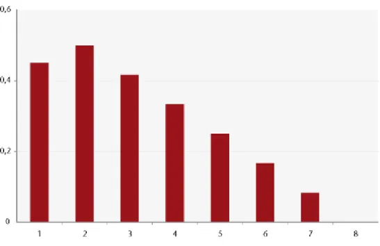
Calibration of fiscal policy parameters determines the duration impact of fiscal policy on GDP. We calibrate the effective fiscal impulse to return to 0 in seven years in normal times,
i.e. when the output gap is close to 0 (see Figure 4). Indeed the effective fiscal impulse also depends on the value of the ex ante instantaneous fiscal multiplier , which can vary over time according to the output gap. More precisely, we define normal times as economic states in which output gap is greater than -1.5% and lesser than 1.5%. In that case, we fix the ex ante instantaneous fiscal multiplier to 0.5 for big countries (Germany, France, Italy and Spain), and to 0.3 for other countries, accounting for the fact that fiscal multipliers are generally smaller for small countries (see the recent estimates by Ilzetsky et al., 2011). When output gap is over 1.5%, the ex ante instantaneous fiscal multiplier linearly decreases to 0, until output gap reaches 6%.
In bad times, the ex ante instantaneous fiscal multiplier increases as output gap deteriorates. We set its maximum value to 2 when output gap reaches -6%.
Figure 4. Effective fiscal impulse in normal times with . following a positive fiscal impulse (1% of GDP)
Source: OFCE.
External trade
We set the sensitivity of imports to output gap equal to the share of imports in country’s GDP. The matrix of trade exchanges between countries comes from the Chelem Database for year 2003.
Table 4. Calibration of the sensitivity of imports to output gap
Austria 0.5 Belgium 0.8 Finland 0.4 France 0.3 Germany 0.4 Greece 0.3 Ireland 0.8 Italy 0.3 Netherlands 0.7 Portugal 0.4 Spain 0.3 Source: OECD Economic outlook 91.
Monetary policy and financial markets
We choose standard values for the Taylor rule. The short term interest rate is bound at 0.05% to account for the zero lower bound on monetary policy. We fix 0.82, a value compatible with a long run nominal interest rate of 4% (see Shiller, 1979, or Fuhrer and Moore, 1995).
Table 5. Calibration of monetary policy parameters
∗
0.5 0.5 2% 0.05%
Prices
Values for and are standard in empirical literature on New Keynesian Hybrid Phillips curve estimates (Rudd and Whelan, 2006; Paloviita, 2008).
Table 6. Calibration of Phillips curve and expected inflation parameters
0.5 0.1 0.1 -0.8 Source: iAGS Model, OFCE.
4. The actual consolidation path is ill-designed
Starting from this, we analyze the sustainability of public finances as well as the output losses of the current path of consolidation. The results of this baseline scenario is illustrated in Table 4 (see box 1 for a description of the main underlying hypotheses). In the baseline, we simulate the path of public debt levels (expressed in percentage points of GDP) until 2032, which is the horizon of the 1/20th debt rule incorporated in the revised SGP and in the
Fiscal Compact. The simulated path of public debt levels depends on the fiscal impulses which have been forecast in the euro area from 2013 to 2015. By assumption at this stage, we assume zero fiscal impulses beyond 2016.
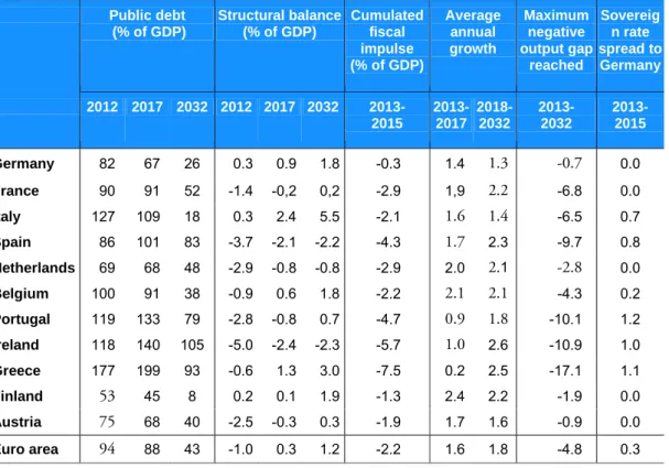
The first six columns report the public debt and the structural balance respectively in 2012, 2017 (5-year horizon) and 2032 (20-year horizon). The cumulated fiscal impulse for 2013-2015 sums up the short term fiscal stance in the euro area as it cumulates forecast variations in structural primary government spending and taxes11. We report the average annual growth rate of real GDP for 2013-2017 and 2018-2032, and the sovereign interest rate spread over Germany for 2013-2015.
Table 4 reports how tough austerity will be all over the euro area: between 2013 and 2015, all MS except Germany and Finland will achieve cyclically-adjusted primary improvements in their public deficit equal to or above 2% of GDP. Spain, Portugal, Ireland and Greece will make even stronger efforts. This highly contractionary fiscal stance will make it ever harder to achieve an output gap at or above zero in our simulation: all MS will have to wait until 2019 (Austria, Finland), 2020 (Germany, France, Italy, Spain, Portugal) or 2021 to close the output gap. Meanwhile, the aggregate euro area GDP will plummet to a maximum negative output gap of almost -5%. Hence, the cumulated fiscal impulse, starting already from negative output gaps for which fiscal multiplier effects are strong, will lead to gloomy prospects for the entire euro area. Germany and Austria will be exceptions, since
they will face almost no further real cost with their forecast fiscal strategy thanks to milder consolidation plans.
Table 4. Baseline scenario
Public debt (% of GDP)
Structural balance (% of GDP)
Cumulated fiscal impulse (% of GDP)
Average annual growth Maximum negative output gap reached Sovereig n rate spread to Germany
2012 2017 2032 2012 2017 2032 2013-2015 2013-2017 2018-2032 2013- 2032 2013- 2015
Germany 82 67 26 0.3 0.9 1.8 -0.3 1.4 1.3 -0.7 0.0
France 90 91 52 -1.4 -0,2 0,2 -2.9 1,9 2.2 -6.8 0.0
Italy 127 109 18 0.3 2.4 5.5 -2.1 1.6 1.4 -6.5 0.7
Spain 86 101 83 -3.7 -2.1 -2.2 -4.3 1.7 2.3 -9.7 0.8
Netherlands 69 68 48 -2.9 -0.8 -0.8 -2.9 2.0 2.1 -2.8 0.0
Belgium 100 91 38 -0.9 0.6 1.8 -2.2 2.1 2.1 -4.3 0.2
Portugal 119 133 79 -2.8 -0.8 0.7 -4.7 0.9 1.8 -10.1 1.2
Ireland 118 140 105 -5.0 -2.4 -2.3 -5.7 1.0 2.6 -10.9 1.0
Greece 177 199 93 -0.6 1.3 3.0 -7.5 0.2 2.5 -17.1 1.1
Finland 53 45 8 0.2 0.1 1.9 -1.3 2.4 2.2 -1.9 0.0
Austria 75 68 40 -2.5 -0.3 0.3 -1.9 1.7 1.6 -0.9 0.0
Euro area 94 88 43 -1.0 0.3 1.2 -2.2 1.6 1.8 -4.8 0.3
Sources : Eurostat, iAGS model.
Real divergence across euro area member states under this scenario will thus widen: Greece will hit the floor with a massive output gap of -17%. Ireland, Spain and Portugal will face substantial losses with output gaps reaching abnormal levels around -10%, and France and Italy will be quite harshly hit, touching the ground at -7% after austerity measures are implemented.
This multi-speed euro area in terms of output losses will also be reflected in structural balances and public debt ratios. In 2017, despite substantial fiscal efforts, Spain, the Netherlands, Portugal and Ireland will not be able to bring their cyclically-adjusted deficit under 0.5% of GDP. Spain, Portugal and Ireland will also not be able to reach the public-debt-to-GDP threshold of 60% of GDP by 2032. The case of Greece is interesting, in this respect: it would not achieve this threshold either, despite an extraordinary structural surplus of 3% of GDP and an outstanding negative fiscal impulse of 7.5% of GDP between 2013 and 2015. Fiscal efforts by this country will not be sufficient to achieve the debt target, due to a deflation between 2014 and 2018 which increases real interest rates.
Another striking result with our simulations is the degree of excess austerity implemented by most countries reaching lower debt ratio at the 5-year horizon. Though European rules require only a maximum deficit of 0.5% of GDP, Germany, Italy, Belgium, Greece and Finland achieve structural surpluses. This clearly indicates that there is leeway to perform less restrictive fiscal policies without breaching EU fiscal rules, as for these countries the debt-to-GDP ratio is below 60% of GDP in 2032.
Finally, this baseline scenario questions the issue of public debt sustainability in the euro area. Consistently with the new fiscal framework, it seems relevant to fix a 20-year horizon for assessing dent sustainability. The simulations are then carried over this horizon.
It must be acknowledged that this issue of public debt sustainability is theoretically and empirically unsettled, between promoters of investigating the statistical properties of public finances' variables on the one hand, and, on the other hand, promoters of a "return to economic thinking" (Bohn, 2007). Stated briefly, sustainability refers to the ability of the general government to pay back the domestic public debt. This ability depends on the future available scope for spending cuts and tax hikes, but also on future economic growth.
In our simulations, the public debt sustainability is assessed regarding the ability of countries to meet the objective of bringing back the debt ratio to 60 % of GDP by 2032. Though some countries in our baseline simulations do not reach this 60% threshold, it is noticeable that they achieve substantial reductions in public debt-to-GDP ratios. For instance, Greece would halve its ratio and Ireland's debt would decrease by 35 percentage points of GDP between 2017 and 2032. This downward trend in public debt implies enhanced debt sustainability stricto sensu. However the social costs as well as the cost in terms of fiscal balance could make this adjustment unrealistic. For Greece, Italy, Portugal and Belgium, it would indeed require structural primary surpluses above 3% of GDP for many years, which have rarely been achieved in history of fiscal consolidation. Debt sustainability is a relative concept and may only be assessed regarding the cost of achieving it.
However, our simulations also show that the long-run debt-to-GDP ratio in many euro area MS is astonishingly low: 26% in Germany, 18% in Italy, even 8% in Finland. It questions the relevance of fiscal austerity in these countries, because public bonds are highly demanded on financial markets, especially "risk-free" bonds like German Bunds. For this reason, it is highly probable that this baseline scenario goes too far in terms of fiscal sustainability in most euro area countries. To sum up, this scenario considers fiscal restrictions that go beyond the requirements of fiscal sustainability, beyond the requirements of EU fiscal rules and beyond the social resilience of European citizens.
The first variant that we introduce in the baseline scenario refers to "fiscal sustainability" stemming from EU treaties and regulations. Sustainability refers here to the ability of EU MS to converge towards a debt target of 60% of GDP. Therefore, we compute simulations that aim at gauging if all countries can attain the public debt target in 2032. We calculate a sequence of fiscal impulses over 2015-2032 that achieve the target, assuming that fiscal impulses for the years 2013 to 2015 are left unchanged. For simplicity, we set fiscal
impulses at -0.5 or +0.5 depending on the gap vis-à-vis the target: the fiscal impulse is positive (resp. negative) if actual debt is above (resp. below) the target. The cumulated fiscal impulse is larger than in the baseline scenario for countries which cannot achieve 60% in this scenario, whereas it is lower for the other countries. For the last group of countries, we gather some pieces of information as regards the margins for manoeuvre for future fiscal policy. Structural balance and average annual growth also indicate what would be the costs or gains in terms of fiscal adjustment and impact on economic activity of sticking to the debt target at 20-year horizon.
The question of fiscal sustainability is crucial for Greece, Ireland, Portugal and Spain since they do not attain this targeted level of debt in the baseline scenario, whereas the question of the costs of fiscal retrenchment is crucial for countries that go beyond the requirements of EU fiscal legislation in the baseline scenario.
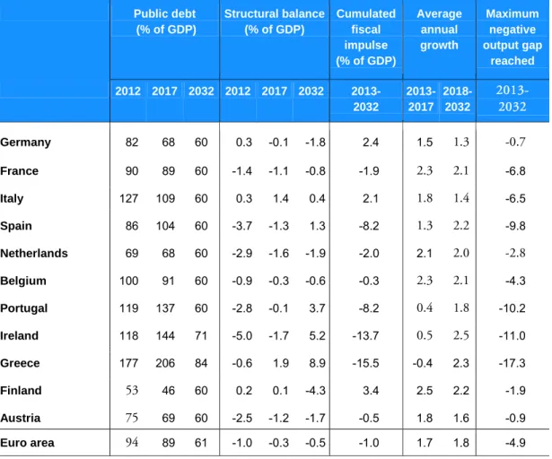
Table 5 sums up the simulation results where we add further consolidation of 0.5 point of GDP per year from 2016 in order to assess whether the 60 % debt ratio would be meet. Striking results are threefold. First, two countries—Ireland and Greece—are still unable to achieve the debt-to-GDP target. It does not preclude fiscal sustainability per se, but it entails further social unsustainability of public finances: the fiscal stance over the period 2013-2032 produces a cumulative fiscal impulse which is highly negative and twice as high (in absolute values) as in the baseline scenario. Such a fiscal stance is entirely unrealistic and inefficient: economic growth in the medium-run would be lowered substantially, and the maximum negative output gap would be even larger. This outcome ensues from the high value of the fiscal multiplier when the output gap is strongly negative, from inertial processes in economic growth once hysteresis is introduced, and from the relatively insufficient decrease in real interest rates, since these two countries suffer from low or negative inflation rates until 2020.
Second, Spain and Portugal achieve the debt target in 2032, but under substantially more restrictive fiscal stances. Fiscal adjustment under such conditions seems unrealistic and unreasonable: between 2013 and 2017, both countries would experience slower economic growth than in the baseline, hence postponing until 2025 (Portugal) and 2027 (Spain) the return to a zero output gap.
Third, countries with public debt levels below the debt target in 2032 have fiscal leeway: indeed, the cumulated fiscal impulse improves by 2.7 percentage points in Germany, 1 in France, 4.2 in Italy, 5.7 in Finland and 1.4 in Austria in this scenario compared to the baseline. Despite fiscal leeway and relatively high fiscal multipliers in the short run, the net gain in terms of economic growth is very small, however. The reason lies in the trade interactions within the euro zone: the enlarged margins for manoeuvre for some countries are compensated by the larger real difficulties incurred by the implementation of a more restrictive fiscal stance in Southern countries and Ireland.
Table 5. Is it possible to reach the target of 60% in 2032 and what is the cost incurred in terms of growth?
Public debt (% of GDP)
Structural balance (% of GDP)
Cumulated fiscal impulse (% of GDP)
Average annual growth
Maximum negative output gap
reached
2012 2017 2032 2012 2017 2032 2013- 2032
2013-2017
2018-2032
2013-
2032
Germany 82 68 60 0.3 -0.1 -1.8 2.4 1.5 1.3 -0.7
France 90 89 60 -1.4 -1.1 -0.8 -1.9 2.3 2.1 -6.8
Italy 127 109 60 0.3 1.4 0.4 2.1 1.8 1.4 -6.5
Spain 86 104 60 -3.7 -1.3 1.3 -8.2 1.3 2.2 -9.8
Netherlands 69 68 60 -2.9 -1.6 -1.9 -2.0 2.1 2.0 -2.8
Belgium 100 91 60 -0.9 -0.3 -0.6 -0.3 2.3 2.1 -4.3
Portugal 119 137 60 -2.8 -0.1 3.7 -8.2 0.4 1.8 -10.2
Ireland 118 144 71 -5.0 -1.7 5.2 -13.7 0.5 2.5 -11.0
Greece 177 206 84 -0.6 1.9 8.9 -15.5 -0.4 2.3 -17.3
Finland 53 46 60 0.2 0.1 -4.3 3.4 2.5 2.2 -1.9
Austria 75 69 60 -2.5 -1.2 -1.7 -0.5 1.8 1.6 -0.9
Euro area 94 89 61 -1.0 -0.3 -0.5 -1.0 1.7 1.8 -4.9
Sources : Eurostat, iAGS model.
Box 1: Main hypotheses for the baseline simulations
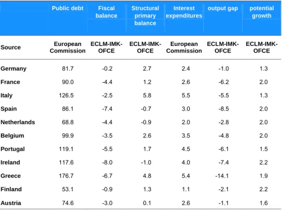
Simulations begin in 2013. To do so, we need to set some starting point values in 2012 for a set of determinant variables. Output gaps for 2012 come from ECLM-IMK-OFCE forecasts. Potential growth for the baseline potential GDP is based on Johansson et al. (2012) projections (see Table 1). Concerning fiscal policy and budget variables, the main hypotheses are as follows:
— The public debt in 2012 comes from the European Commission’s autumn 2012 forecast;
— We use the ECLM-IMK-OFCE forecasts for fiscal balance in 2012;
— We use the European Commission’s autumn 2012 forecast of interest expenditures for 2012; combined with ECLM-IMK-OFCE forecasts of output gaps in 2012, and model
estimates of the cyclical part of the fiscal balance, it gives the structural primary balance for 2012;
— Fiscal impulses come from ECLM-IMK-OFCE forecasts for 2013 (see Table 2). For 2014-2015, we use fiscal impulses implied by the Stability and Growth Pact reported in the “Assessment of the 2012 national reform programme and stability programme” for each country.
— Sovereign spreads come from ECLM-IMK-OFCE forecasts for 2013-2015 (see Table 3). We made the hypothesis that the ECB program of unlimited debt buying on the secondary market (Outright Monetary Transactions) is effective and achieves its goal to bring down interest rates for Italy and Spain. Regarding countries relying on the ESM for debt financing, we assume that Ireland will get direct access to financial markets as of 2014, Portugal as of 2015 and Greece as of 2016.
Table 1. Main hypotheses for 2012 in %
Public debt Fiscal
balance Structural primary balance Interest expenditures
output gap potential growth
Source European Commission ECLM-IMK-OFCE ECLM-IMK-OFCE European Commission ECLM-IMK-OFCE ECLM-IMK-OFCE
Germany 81.7 -0.2 2.7 2.4 -1.0 1.3
France 90.0 -4.4 1.2 2.6 -6.2 2.0
Italy 126.5 -2.5 5.8 5.5 -5.5 1.3
Spain 86.1 -7.4 -0.7 3.0 -8.5 2.0
Netherlands 68.8 -4.4 -0.9 2.0 -2.8 2.0
Belgium 99.9 -3.5 2.6 3.5 -4.8 2.0
Portugal 119.1 -5.5 1.7 4.5 -6.1 1.5
Ireland 117.6 -8.0 -1.0 4.0 -7.4 2.2
Greece 176.7 -6.7 4.8 5.4 -14.1 1.9
Finland 53.1 -0.9 1.3 1.1 -2.1 2.2
Austria 74.6 -3.0 0.1 2.6 -1.1 1.6
Sources: European Commission, ECLM-IMK-OFCE forecasts.
Table 2. Fiscal impulse in % of GDP
2013 2014 2015
Germany 0.0 -0.3 0.0
France -1.8 -0.6 -0.5
Italy -2.1 0.0 0.0
Spain -2.5 -1.2 -0.6
Belgium -0.8 -0.6 -0.8
Portugal -2.9 -0.6 -0.2
Ireland -1.8 -2.1 -1.8
Greece -3.9 -2.7 -0.9
Finland -1.3 0.0 0.0
Austria -0.9 -0.3 -0.6
Sources: ECLM-IMK-OFCE forecasts.
Table 3. Sovereign spreads relative to German interest rate on public debt in %
2013 2014 2015
Germany 0.0 0.0 0.0
France 0.1 0.0 0.0
Italy 1.3 0.8 0.0
Spain 1.5 0.8 0.0
Netherlands 0.1 0.0 0.0
Belgium 0.5 0.1 0.0
Portugal 1.4 1.2 1.0
Ireland 1.4 1.5 0.0
Greece 1.4 1.2 0.9
Finland 0.0 0.0 0.0
Austria 0.0 0.0 0.0
Sources: ECLM-IMK-OFCE forecasts.
5. Searching for a less costly alternative strategy
In this section, we address the issue of the opportunity to soften (or spread) and to delay the consolidation. The scope of alternative scenarios is inevitably infinite and any scenario reducing the strength of fiscal consolidation would improve growth but it may also undermine the sustainability of public debt12. The identification of any alternative strategy is then fundamentally based on a trade-off between growth and debt. The stronger is the consolidation, the costlier it is in terms of output losses and the more debt is reduced unless the size of the fiscal multiplier exceeds 2 (see Part 1 of this report). Conversely, a more cautious path of consolidation may delay the reduction of debt but it would improve growth.
The aim of this study is then to identify an efficient strategy, that is a strategy reducing the output losses of consolidation while keeping constant the objective for public debt. In theory, it resumes to an optimal control problem which may be solved using the appropriate algorithm. But there is no guarantee that the optimal solution may one that can be implemented in practice. This is why we are seeking a solution compatible with the spirit of the various fiscal rules governing EMU member states. Taking into account the objective of the TSCG, we maintain the objective for public debt at 60% of GDP in 2032. We also claim that the current rules leave leeway for an alternative strategy. Firstly, the minimum annual improvement of the cyclically-adjusted balance (net of one-off measures) of 0.5% of GDP is held to be consistent with the needed correction of the excessive deficit. In addition most EMU countries have scope to invoke the exceptional circumstances escape clause as they face “an unusual event” (see section 1 above).
i) Starting from this, we first consider the case where the consolidation is spread out from 2013 onwards. We implement a yearly consolidation of 0.5 point of GDP consistent with the objective of 60 % of debt in 2032 as identified in the previous section. The main difference with the scenario described in Table 5 is that we replace the scheduled consolidation path from 2013 until 2015 (see Table 2 in box 1) by a consolidation, which does not exceed 0.5% of GDP from 2013 until 2032. For those countries (Greece and Ireland) where the 60% debt ratio was not reached in 2032, we implement the same spread consolidation strategy from 2013 to 2032. The aim here is simply to check whether a milder consolidation would reduce the output losses while maintaining the objective of bringing the debt ratio back towards 60% in twenty years. In such a case, it must be noted that the strategy is not differentiated as the yearly fiscal stance will be the same for each country. The only difference is that the consolidation is stopped as soon as the 60% debt ratio is reached. In each case, we assess whether this alternative strategy leads to a reduction in the output losses. For Greece and Ireland, we may also compare the level of public debt in 2032.
ii) In a second step, we proceed the same way except that consolidation is also delayed. The start of the consolidation is chosen according to the date where it is the most efficient (see box 2 for detailed explanations on the way this optimal date is chosen).
Is it more appropriate to spread the consolidation?
The efficiency of such a strategy, where austerity is softened but not delayed, should first be assessed regarding the average growth over the period. From this, it appears clearly that on the 2013-2017 period, the average growth for the euro area as a whole is 0.6 point higher (Table 6) than in a scenario where the consolidation is not spread over time and corresponds to what has been announced by the national governments in their convergence plans (in these plans, consolidation occurs when it hurts more, that is when
the size of the fiscal multiplier is the highest). Consolidation would be spread meaning that a larger share of the consolidation would be implemented when the output gap has recovered. The negative impact on growth would then be reduced.
The main reason for this result is that there would be less consolidation since consolidation is more efficient (in terms of debt reducing) when the output gap is closed. The most striking difference is identified for Greece where the average growth between 2013 and 2017 is 3.6 points higher than if the current expected consolidation path is implemented. Besides, this strategy would enable Greece to reduce debt in 2032 more significantly even though the cumulated fiscal stance would be loosened, amounting to -3.3 points of GDP in the spread consolidation scenario against -15.5 points otherwise. It must however be noticed that from 2018 until 2032, growth would be slightly reduced in the scenario where consolidation is softened since it also involves that it is spread over a longer period of time . The situation of Greece is the most symptomatic of this ill-designed consolidation. Actually, the Greek public deficit results mainly from cyclical effects and interest payments. The structural deficit amounts to -0.6 % of GDP for 2012 which is already near the so-called "golden rule" enacted in the fiscal compact. Then it is urgent for Greece to reduce the path of consolidation. This is the only condition for growth to resume, which may contribute to the reduction of the cyclical-deficit. Such a strategy would also avoid a deflation episode in Greece. The real interest rate between 2013 and 2017 would be indeed 2 points less than in the scenario where the fiscal stance is what is currently scheduled in the convergence programme. Finally, spreading the consolidation would lead to structural surplus of 0.8% for Greece in 2017 instead of 1.9 % for the scenario where consolidation is not spread. By 2032, the structural balance would reach 3.5% of GDP, which is still quite high relative to historical standards but it is nevertheless significantly less than in the baseline scenario( 8.9% of GDP).
If we turn to the other countries, results are in the same vein even if the contrast is less striking. Thus, the average growth for the 2013-2017 period would be higher for all euro area countries except Austria, where there would no changes in growth. For the other countries, the benefit would range from 0.1 point in Germany to 2.2 points in Ireland. Portugal, Spain and Italy would be the countries benefiting the most from such a strategy.
Table 6. Is it more appropriate to spread fiscal impulses over time ?
Public debt (% of GDP)
Structural balance (% of GDP)
Cumulated fiscal impulse (% of GDP)
Average annual growth Maximum negative output gap reached
2012 2017 2032 2012 2017 2032 2013- 2032 2013-2017 2018-2032 2013- 2032
Germany 82 72 60 0.3 -1.1 -1.3 1.8 1.6 1.3 -0.5
France 90 86 60 -1.4 -1.0 -0.9 -1.3 2.6 2.1 -4,7
Italy 127 104 60 0.3 -0.6 0.9 2.4 2.6 1.2 -2.7
Spain 86 96 60 -3.7 -2.6 0.8 -6.0 2.5 2.1 -6.3
Netherlands 69 69 60 -2.9 -1.5 -1.9 -1.9 2.2 2.0 -2.3
Belgium 100 89 60 -0.9 -1.0 -0.7 0.4 2.7 2.0 -2.9
Portugal 119 119 60 -2.8 -0.9 1.9 -3.9 1.9 1.6 -4.2
Ireland 118 125 67 -5.0 -3.7 3.9 -9.5 2.7 2.3 -5.6
Greece 177 150 60 -0.6 0.8 3.5 -3.3 3.2 2.0 -8.0
Finland 53 54 60 0.2 -2.1 -3.0 2.0 2.7 2.1 -1.1
Austria 75 71 60 -2.5 -1.5 -1.5 -0.7 1.8 1.6 -0.8
Euro area 94 90 62 -1.0 -1.3 -0.4 -0.4 2.3 1.8 -3.1
Sources : Eurostat, iAGS model.
Box 2: An algorithm for a “well balanced austerity”
Simulating a (small, negative) fiscal impulse on a certain year (and no fiscal impulse for any other year) and then running the model enables to determine the level of debt in 2032. We may then compare the path of debt reduction with the alternative path of neutral budgetary policy (figure 1). It is inducing a debt reduction (as compared to the reference path) if multipliers are not too large and sufficient time is left for debt reduction to occur. As the fiscal impulse is small this is an approximation of the first derivative of debt to GDP ratio 20 years from now relative to impulse in any year from now. If the model is linear (no hysteresis and fixed fiscal multiplier), then, the graph is independent of initial conditions and derivatives are independent of the size of the impulse. If not, then the graph is a linearization of the problem on a current state of the economy (described by initial conditions or state variable at a given period) and for a small shock.
Things get a bit more complicated when one considers that the underlying dynamic for graph1 is more realistic and allows for some non linearity (hysteresis and time-varying fiscal multiplier). Figure 2 is based on a cycle (output gap) dependent multiplier and includes negative output gaps described above as initial conditions to the system. In such a model and initial conditions, multipliers are higher than a given critical value for which it is equivalent to engage fiscal restriction now or one year later, for a given amount of debt reduction. Thus postponing the negative fiscal impulse by one year or more is more efficient for debt reduction.
Figure 1. Debt reduction in 2032 for a 1.0 fiscal impulse on a given year
Figure 2. Debt reduction in 2032 for a 1.0 fiscal impulse on a given year, non linear model
Cycle dependant multiplier and hysteresis
The algorithm is then simple: given an initial debt to GDP ratio, given a timeframe for reducing debt to 60% (20 years), given a maximum fiscal impulse of Imax=±0.5, Figure 1 is
used to select the timing of the first fiscal impulse based on the maximum efficiency of fiscal impulse. Figure 1 suggest that austerity is more efficient (in terms of debt reduction) when the negative fiscal impulse is done in the first period, and thus suggest a pattern of fiscal impulses of Imax for the first years until it is sufficient to bring down debt to target
level. Such an algorithm selects the more parsimonious sequence of fiscal impulses to reduce debt.
Following dynamics represented by Figure 2, the afore-mentioned algorithm states that fiscal impulses should not start in 2013 in most countries. The necessary sequence for debt reduction would thus follow a pattern of no impulse before the inflexion date and Imax
for some time from the inflexion date, as long as necessary to reduced debt to 60% in 2032. The Table 4 indicates the date where it is optimal to start the consolidation according to these calculations.
It may happen—as we describe below- that the debt target is not achievable through this process. This means that given Imax and the underlying dynamic of the economy, the debt
target is not sustainable.. Then, it may be computed for instance what Imax would allow for
the 60% debt-to-GDP ratio to be reachable.
Following the algorithm described above, we calculate the best timing to engage in fiscal restriction. We show that in case of a large negative output gap, waiting is more efficient for debt reduction, due to the higher current value of the fiscal multiplier. Accordingly, we find that there are 6 countries for which it would be optimal to delay the start of the consolidation (Table 7). The model emphasizes that the wider is the output gap, the more it is optimal to postpone consolidation. The efficiency of the consolidation would be increased in so far as time would be given for growth to recover. Such a strategy implicitly boils down to a 2-step approach. It stresses that it is first needed to let the cyclically-adjusted deficit be reduced in line with the closing of the output gap. Then, once the output gap is closed, it becomes more efficient to undertake the fiscal consolidation per se, that is the needed reduction of the structural deficit. Thus, for Greece, it would be more efficient to start the consolidation from 2017. For France, Spain and Ireland, it would be better to implement a neutral fiscal policy until 2016. Finally, for Netherlands and Portugal, the reduction of debt would be optimized if consolidation started in 2015.
Comparing Table 7 to Table 5, we show that delaying the fiscal consolidation leads to a higher average growth in 2013-2017 in concerned countries, and for the euro zone as a whole (2.4% for the 2013-2017 period, against 1.7% without delaying the adjustment). Greece is again the country which would benefit most from delaying its fiscal consolidation. Yearly average growth would be 4.5 points higher between 2013 and 2017. Then, as the output gap would close more rapidly, the average growth would be slightly inferior from
2018 to 2032. It must also be noticed that postponing consolidation would achieve the same target for debt, relatively to the situation where consolidation is only spread over time, with a cumulated fiscal impulse that would be only half as large. This is largely explained by the cycle-dependent multiplier, which makes austerity less painful since it is postponed until the multiplier reaches a lower value. Similarly, Portugal, Spain, and Ireland combine a gain of 0.5 to 0.6 point of growth on average over the same period when they delay fiscal consolidation and implement a greater reduction in their structural deficit.. For France, the average growth would be 0.2 point higher compared to the situation where the consolidation is only spread. This improvement would stem from the better prospects of trade partners within the euro area. It remains to be said that this mild improvement would give a net gain of 0.5 point in comparison with the baseline situation where the French government sticks to its current fiscal commitments.
For Austria and Germany, the alternative strategy would not entail a significant lower consolidation. Then, on the one side, those countries would benefit from a stronger growth in the rest of the euro area. But, on the other side, interest rates would be higher as a result of a relative tightening of monetary policy, through the Taylor rule. For Germany, real interest rates would on average amount to 1.7% when consolidation is delayed in all other euro area countries against 1% in the scenario where the current commitments are respected.
Table 7. Is it more appropriate to postpone the start of fiscal adjustment
Public debt (% of GDP)
Structural balance (% of GDP)
Cumulated fiscal impulse (% of GDP)
Average annual growth Maximum negative output gap reached Starting date of fiscal impulses (sign of FI) 2012 2017 2032 2012 2017 2032 2013-
2032 2013-2017 2018-2032 2013-2032
Germany 82 74 60 0.3 -1.3 -1.1 1.6 1.6 1.3 -0.7 2013 (+)
France 90 86 60 -1.4 -1.2 -0.8 -1.1 2.8 2.1 -4,0 2016 (-)
Italy 127 107 60 0.3 -0.7 1.3 1.9 2.4 1.3 -3.0 2013 (+)
Spain 86 95 60 -3.7 -4.0 2.4 -7.3 3.1 1.9 -5.7 2016 (-)
Netherlands 69 72 60 -2.9 -2.1 -1.6 -2.1 2.3 2.0 -2.1 2015 (-)
Belgium 100 90 60 -0.9 -1.3 -0.5 0.1 2.7 2.0 -3.2 2013 (+)
Portugal 119 116 60 -2.8 -1.7 1.9 -3.3 2.4 1.6 -3.3 2015 (-)
Ireland 118 123 78 -5.0 -5.1 2.7 -8.0 3.2 2.2 -4.7 2016 (-)
Greece 177 141 60 -0.6 -0.3 2.8 -1.5 4.1 1.9 -7.1 2017 (-)
Finland 53 56 60 0.2 -2.3 -2.8 1.8 2.6 2.2 -1.3 2013 (+)
Euro area 94 88 60 -1.0 -1.6 -0.1 -0.7 2.4 1.7 -2.9 Sources : Eurostat, iAGS model.
Appendix
“Well-balanced austerity” and sensitivity to baseline hypotheses
As we have seen before, the path of fiscal consolidation determines the sustainability of public debt, and a "well-balanced" austerity helps achieving the target of 60% in 2032 without huge losses in term of growth. However, such simulations hinge on the assumption that negative output gaps are large in most countries of the euro area (see Table 1 in Box). Results strongly depend on this assumption since it implies high fiscal multipliers, and postponing the fiscal adjustment is a way to reduce them. The other strong assumption concerns yield spreads. In the baseline scenario, we assumed that the OMT program of ECB would succeed in diminishing Italian and Spanish sovereign interest rates, helping these countries to achieve sustainability of their public debt. In this part, we discuss these two assumptions.
A.1. Closed output gaps in 2012
The implications of a low output gap in our model are twofold: on the one hand, spontaneous growth is strengthened in order to close the output gap, and on the other hand, fiscal multipliers are higher, hampering growth when fiscal impulses are negative. The final outcome in term of growth is therefore ambiguous, and depends on the level of the output gap and on the size of the fiscal adjustment performed. If, in contrast, we assume that we are in a situation of "new normal", characterised by a closed output gap in 2012, average growth during the period 2013-2017 is lower in all countries except Portugal, Ireland and Greece compared to the baseline scenario, which benefit from low fiscal multipliers while making their strong fiscal adjustment (Table 8).
Table 8. What if the Output Gap were zero in 2012 (New normal)
Public debt (% of GDP)
Structural balance (% of GDP)
Cumulated fiscal impulse (% of GDP)
Average annual growth
Maximum negative output gap
reached
2012 2017 2032 2012 2017 2032 2013- 2032
2013-2017
2018-2032
2013-
Germany 82 72 39 0.3 0.0 0.8 -0.3 1.3 1.3 -0.3
France 90 89 75 -4.4 -2.1 -2.1 -2.9 1.7 2.0 -1.2
Italy 127 113 51 -2.5 0.0 2.6 -2.1 1.1 1.3 -1.3
Spain 86 97 105 -7.4 -4.1 -4.6 -4.3 1.6 2.1 -2.0
Netherlands 69 70 64 -4.4 -2.0 -2.2 -2.9 1.8 2.0 -0.8
Belgium 100 93 62 -3.5 -1.4 -0.5 -2.2 1.9 2.0 -0.7
Portugal 119 111 64 -5.5 -0.8 0.9 -4.7 1.4 1.6 -1.1
Ireland 118 118 92 -8.0 -2.9 2.2 -5.7 1.9 2.3 -1.5
Greece 177 140 42 -6.7 1.6 4.5 -7.5 1.8 1.9 -0.6
Finland 53 49 25 -0.9 -0.1 0.4 -1.3 2.1 2.2 -1.5
Austria 75 72 53 -3.0 -1.1 -0.7 -1.9 1.5 1.6 -0.4
Euro area 94 88 61 -3.2 -1.2 -0.5 -4.7 1.5 1.7 -0.9
Sources : Eurostat, iAGS model.
The most striking case is Greece, where GDP growth is on average 1.6 point higher, implying positive inflation rates and much lower real interest rates on average over the period 2013-2017 (1.7% compared to 4.4% in the baseline scenario). Higher growth and lower interest rates lead to a much stronger debt reduction over 20 years: the debt to GDP ratio is back to 42% instead of 93% in the baseline scenario, for the same cumulated fiscal impulse (-7.5%). Portugal and Ireland also end up with lower debt ratios, even if the difference with the baseline scenario is less striking.
This change in the assumption regarding current output gaps makes it clear that the plea for strong and immediate fiscal retrenchment is based upon the existence of a so-called "new normal" path of economic growth. Drawing on such an assumption, the iAGS model reports simulation results which are at odds with the current Greek state of the economy, for instance. The "new normal" assumption is pretty much normative, but it lacks empirical validity.
A.2. Higher spreads over the German sovereign bond yield
To assess the sensitivity of results to this hypothesis, we simulate the path of public debts under the alternative hypothesis that sovereign spreads above the German rate observed in 2012 persist until 2015 (see Table 9). These high spreads, especially for Greece, Portugal and Ireland, imply that these three countries would almost surely stay in the ESM (European Stability Mechanism) until 2015 to fund their debt and deficit.
In this alternative scenario, the average spread over the German rate would be higher for each country except for countries in the ESM. Specifically, we assume that the average