Electronic Supplement for Seismic Tomography of the
Uppermost Inner Core
Scott Burdick, Lauren Waszek, & Vedran Lekic
Supplement A: Damped inversion
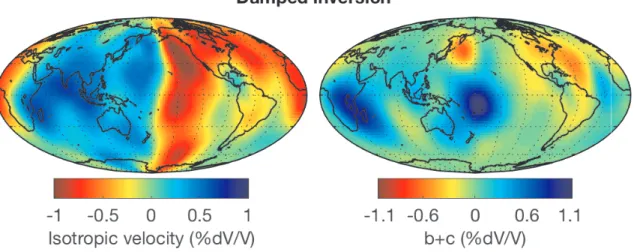
To confirm the accuracy of our forward matrix provide set a point for comparison, we first performed a damped least squares inversion of the residual travel times relative to AK135. The inversion is performed on a 3◦×3◦ grid, and smoothing is applied at a level determined by L-curve test. The resulting model is shown in Figure S1.
The isotropic model exhibits strong hemispheric structure in addition to regional vari-ations on the scale of ∼30◦, particularly in the western hemisphere. The heterogeneity in the eastern hemisphere varies from ∼0.3 %dV/V to∼0.8 %dV/V, while the variation in the west is stronger, about -1.0 %dV/V to 0.1 %dV/V. It should be noted that the locations of near-zero velocity perturbation in the west correspond to the locations without adequate ray coverage.
The isotropic hemisphere boundaries each vary strongly with latitude. The boundary beneath Africa has a westward bulge of 3–5◦ at 30◦S, while the Pacific boundary trends westward from 210◦ to 180◦ between the northern and southern ends of the boundary. As a result of lateral smoothing, the transitions between the hemispheres appear to take place
directions. We find regions of high anisotropy in Africa and the Pacific between 30◦S and the equator, coincident with fast ray paths in the axial direction. Additional regions of slower velocity in the axial direction are recovered beneath the North Atlantic and Japan.
Interpretation of the damped least squares model is complicated by several factors. First, the strength and scale of the structure and sharpness of the hemisphere boundaries is heavily influenced by the choice of damping parameters. Second, for most choices of damping, the imprint of ray coverage remains visible in the model. For instance, the isotropic velocity perturbation is found to be near zero around South America, but this is more easily attributed to lack of ray paths rather than regional structure. Finally, the variation of the boundaries in latitude may reflect variations in ray coverage rather than actual structural changes.
Supplement B: Resolution tests
B.1: Methodology
In order to test the efficacy of the tomographic method and evaluate the relationship of isotropic hemispheric and regional structure with anisotropy, we performed a series of res-olution tests. For each resres-olution test, a synthetic model was created including isotropic velocity and the axial anisotropic parameters b and c. We used one of three possible input models for each in combination: A quasi-hemispheric model with velocity values of ±1.1% dV/V and boundaries at 19◦ and 172◦ longitude, a checkerboard “regional” model with 60◦ wide sine-shaped checks with a maximum variation of ±1.1% dV/V, and a combination model with hemispheres plus checkerboard variations of±0.55% dV/V. We constrain it that
b = c, so the overall amplitude of b+c variations is twice that of the synthetic isotropic model.
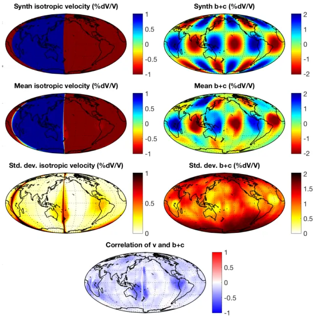
inversion. We then a perform TBI inversion for each synthetic model using the proposal and prior distributions from the data study. Each inversion consists of 20 chains of 500,000 iterations apiece. From the resulting model ensembles, we plot the mean models, standard deviations, and correlations (as in Figure 4) and the probability density functions at constant latitude slices (as in Figure 5).
B.2: Resolution Test Results
Figures S2-S15 show the results of resolution tests for several scenarios: First, we tested purely hemispheric isotropic structure, without regional anisotropy (Figures S2 and S3) and with it (Figures S4 and S5). Next, we tested isotropic structure with both hemispheric and regional variations with no anisotropy (Figures S6 and S7), regional anisotropy (Figures S8 and S9), and hemispheric anisotropy (Figures S10 and S11). Finally, we tested scenarios with no isotropic variations and hemispheric (Figures S12 and S13) and regional anisotropy (Figures S14 and S15).
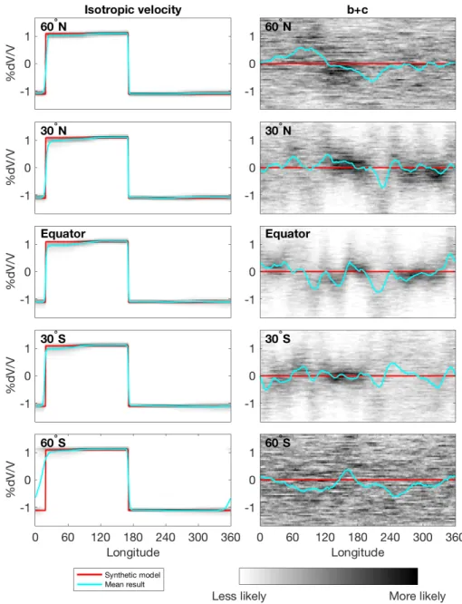
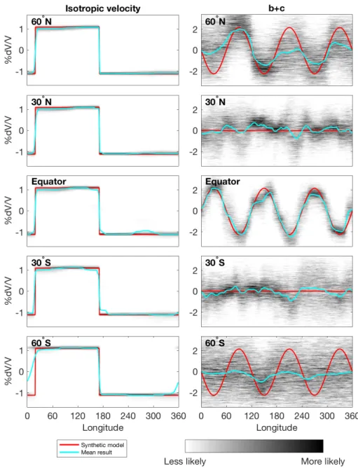
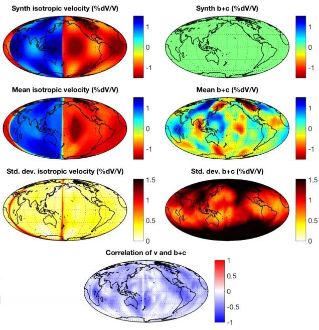
For the tests with b = c = 0 (Figures S2-S3 and S6-S7, strong isotropic variations give rise to small-scale variations in b +c. The amplitude of the variation is stronger for the hemisphere plus regional model Figure S6 than for the purely hemispheric model, but the variations are, in most locations, within 2σ of the true value of b+c = 0. The spurious
b+cvariations are of the same order as the true isotropic heterogeneity (Figure S6) or lower (Figure S2). For the model derived from real data, these variations are four times higher in amplitude, suggesting that they are not entirely due to a mis-assignment of isotropic heterogeneity.
Tests with zero isotropic velocity variation, on the other hand, demonstrate that anisotropic variations are less likely to give rise to isotropic artifacts. For both hemispheric (Figures S12-S13) and regional (Figures S14-S15), the ensemble shows low isotropic variations with a high
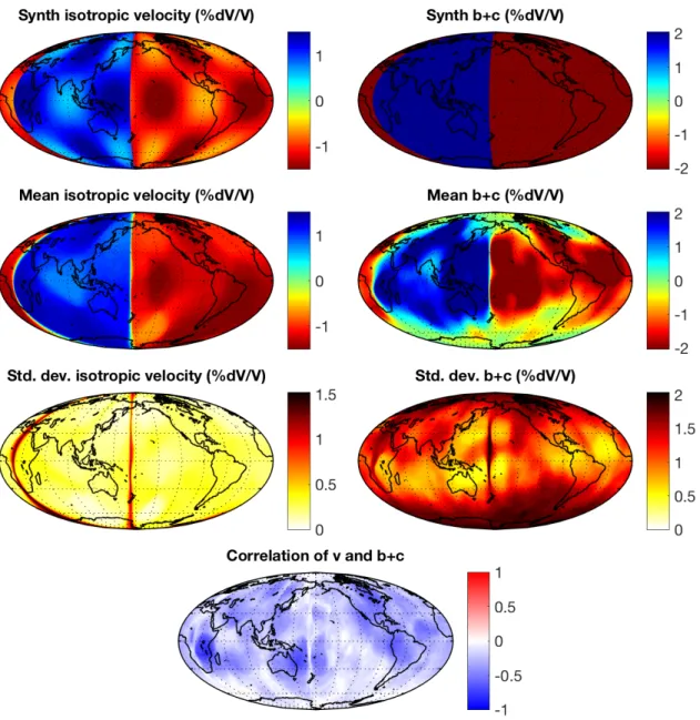
model places the Pacific boundary location with a high degree of certainty, while the African boundary is more uncertain. The mean model shows a gradient in the boundary in the longitude direction, suggesting that this feature in the real data model is driven more by geometry-based uncertainty than by a gradual transition between the hemispheres. Regional variations in both isotropic velocity (e.g. Figure S6) and anisotropy (Figures S4-S5) do have a minor effect on boundary location. These models show an increased uncertainty in boundary location and trade-off with anisotropy, but the mean average boundary location remains accurate.
In models where hemispheric anisotropy is input (Figures S10-S11 and Figures S12-S13), the hemispheres and amplitudes are well-recovered at low latitudes. This suggests that hemispheric variation in anisotropy is either not present in the data or overwhelmed by regional variation.
Figure S1: Lateral variations (in percent) of isotropic VP and anisotropy (b and c terms of
Figure S2: Resolution test for isotropic hemispheres and no anisotropy. Row 1: Input isotropic and b+c models. Row 2: Mean isotropic velocity and b+c. Row 3: Standard deviations of isotropic velocity and b+c. Row 4: Correlation between isotropic velocity and b+c.
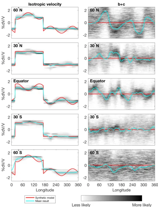
Figure S3: Probability density functions for isotropic velocity (left) and b+c (right) for models in Figure S2 at latitudes indicated by dashed grid lines. Darker grays show values more common in the model ensemble. Cyan lines show mean model values, and red lines show the true input model values.
Figure S4: Resolution test for isotropic hemispheres and regional anisotropic structure. Row 1: Input isotropic and b+c models. Row 2: Mean isotropic velocity and b+c. Row 3: Standard deviations of isotropic velocity and b+c. Row 4: Correlation between isotropic velocity and b+c.
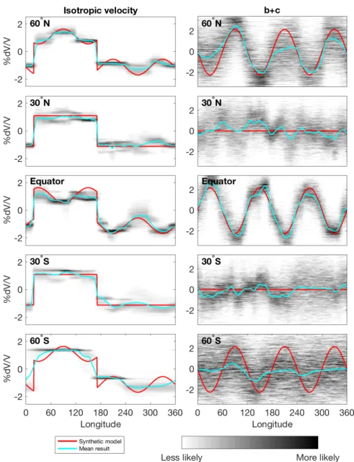
Figure S5: Probability density functions for isotropic velocity (left) and b+c (right) for models in Figure S4 at latitudes indicated by dashed grid lines. Darker grays show values more common in the model ensemble. Cyan lines show mean model values, and red lines show the true input model values.
Figure S6: Resolution test for an isotropic model with hemispheric and regional structure and no anisotropy. Row 1: Input isotropic and b+c models. Row 2: Mean isotropic velocity and b+c. Row 3: Standard deviations of isotropic velocity and b+c. Row 4: Correlation between isotropic velocity and b+c.
Figure S7: Probability density functions for isotropic velocity (left) and b+c (right) for models in Figure S6 at latitudes indicated by dashed grid lines. Darker grays show values more common in the model ensemble. Cyan lines show mean model values, and red lines show the true input model values.
Figure S8: Resolution test for an isotropic model with hemispheric and regional structure and regional anisotropic structure. Row 1: Input isotropic and b+c models. Row 2: Mean isotropic velocity and b+c. Row 3: Standard deviations of isotropic velocity and b+c. Row 4: Correlation between isotropic velocity and b+c.
Figure S9: Probability density functions for isotropic velocity (left) and b+c (right) for models in Figure S8 at latitudes indicated by dashed grid lines. Darker grays show values more common in the model ensemble. Cyan lines show mean model values, and red lines show the true input model values.
Figure S10: Resolution test for an isotropic model with hemispheric and regional structure and hemispheric anisotropy. Row 1: Input isotropic and b+c models. Row 2: Mean isotropic velocity and b+c. Row 3: Standard deviations of isotropic velocity and b+c. Row 4: Correlation between isotropic velocity and b+c.
Figure S11: Probability density functions for isotropic velocity (left) and b+c (right) for models in Figure S10 at latitudes indicated by dashed grid lines. Darker grays show values more common in the model ensemble. Cyan lines show mean model values, and red lines show the true input model values.
Figure S12: Resolution test for a model with hemispheric anisotropy and no isotropic vari-ation. Row 1: Input isotropic and b+c models. Row 2: Mean isotropic velocity and b+c. Row 3: Standard deviations of isotropic velocity and b+c. Row 4: Correlation between isotropic velocity and b+c.
Figure S13: Probability density functions for isotropic velocity (left) and b+c (right) for models in Figure S12 at latitudes indicated by dashed grid lines. Darker grays show values more common in the model ensemble. Cyan lines show mean model values, and red lines show the true input model values.
Figure S14: Resolution test for a model with regional anisotropy and no isotropic variation. Row 1: Input isotropic and b+c models. Row 2: Mean isotropic velocity and b+c. Row 3: Standard deviations of isotropic velocity and b+c. Row 4: Correlation between isotropic velocity and b+c.
Figure S15: Probability density functions for isotropic velocity (left) and b+c (right) for models in Figure S14 at latitudes indicated by dashed grid lines. Darker grays show values more common in the model ensemble. Cyan lines show mean model values, and red lines show the true input model values.