A&A 555, A45 (2013)
DOI:10.1051/0004-6361/201220885 c
ESO 2013
Astronomy
&
Astrophysics
Evolution of CO lines in time-dependent models of protostellar
disk formation
D. Harsono
1,2, R. Visser
3, S. Bruderer
4, E. F. van Dishoeck
1,4, and L. E. Kristensen
1,51 Leiden Observatory, Leiden University, PO Box 9513, 2300 RA Leiden, The Netherlands e-mail:[email protected]
2 SRON Netherlands Institute for Space Research, PO Box 800, 9700 AV Groningen, The Netherlands 3 Department of Astronomy, University of Michigan, 500 Church Street, Ann Arbor, MI 48109-1042, USA 4 Max-Planck-Institut für extraterrestrische Physik, Giessenbachstrasse 1, 85748 Garching, Germany 5 Harvard-Smithsonian Center for Astrophysics, 60 Garden Street, Cambridge, MA 02138, USA
Received 11 December 2012/Accepted 16 April 2013
ABSTRACT
Context.Star and planet formation theories predict an evolution in the density, temperature, and velocity structure as the envelope collapses and forms an accretion disk. While continuum emission can trace the dust evolution, spectrally resolved molecular lines are needed to determine the physical structure and collapse dynamics.
Aims.The aim of this work is to model the evolution of the molecular excitation, line profiles, and related observables during low-mass star formation. Specifically, the signatures of disks during the deeply embedded stage (Menv>M) are investigated.
Methods.The semi-analytic 2D axisymmetric model of Visser and collaborators has been used to describe the evolution of the density, stellar mass, and luminosity from the pre-stellar to the T-Tauri phase. A full radiative transfer calculation is carried out to accurately determine the time-dependent dust temperatures. The time-dependent CO abundance is obtained from the adsorption and thermal desorption chemistry. Non-LTE near-IR (NIR), far-IR (FIR), and submm lines of CO have been simulated at a number of time steps. Results.In single dish (10−20beams), the dynamics during the collapse are best probed through highly excited13CO and C18O lines, which are significantly broadened by the infall process. In contrast to the dust temperature, the CO excitation temperature derived from submm/FIR data does not vary during the protostellar evolution, consistent with C18O observations obtained withHerscheland from ground-based telescopes. The NIR spectra provide complementary information to the submm lines by probing not only the cold outer envelope but also the warm inner region. The NIR high-J(≥8) absorption lines are particularly sensitive to the physical structure
of the inner few AU, which does show evolution. The models indicate that observations of13CO and C18O low-Jsubmm lines within a≤1(at 140 pc) beam are well suited to probe embedded disks in Stage I (Menv<M) sources, consistent with recent interferometric observations. High signal-to-noise ratio subarcsec resolution data with ALMA are needed to detect the presence of small rotationally supported disks during the Stage 0 phase and various diagnostics are discussed. The combination of spatially and spectrally resolved lines with ALMA and at NIR is a powerful method to probe the inner envelope and disk formation process during the embedded phase.
Key words.stars: formation−accretion, accretion disks−radiative transfer−astrochemistry−methods: numerical
1. Introduction
The semi-analytical model of the collapse of protostellar en-velopes (Shu 1977; Cassen & Moosman 1981; Terebey et al. 1984) has been used extensively to study the evolution of gas and dust from core to disk and star (Young & Evans 2005;Dunham et al. 2010;Visser et al. 2009). Others have explored the effects of envelope and disk parameters representative of specific evo-lutionary stages on the spectral energy distribution (SED) and other diagnostics (Whitney et al. 2003; Robitaille et al. 2006, 2007;Crapsi et al. 2008;Tobin et al. 2011). These studies have focused primarily on the dust emission and its relation to the physical structure. On the other hand, spectroscopic observa-tions toward young stellar objects (YSOs) performed by many ground-based (sub)millimeter and infrared telescopes also con-tain information on the gas structure (Evans 1999). The molec-ular lines are important in revealing the kinematical information of the collapsing envelope as well as the physical parameters of
Appendices are available in electronic form at
http://www.aanda.org
the gas based on the molecular excitation. TheHerschelSpace Observatory and the Atacama Large Millimeter/submillimeter Array (ALMA) provide new probes of the excitation and kine-matics of the gas on smaller scales and up to higher tempera-tures than previously possible. It is therefore timely to simulate the predicted molecular excitation and line profiles within the standard picture of a collapsing envelope. The aim is to identify diagnostic signatures of the different physical components and stages and to provide a reference for studies of more complex collapse dynamics.
A problem that is very closely connected to the collapse of protostellar envelopes is the formation of accretion disks. The presence of embedded disks was inferred from the excess of continuum emission at the smallest spatial scales through in-terferometric observations (e.g.Keene & Masson 1990;Brown et al. 2000;Jørgensen et al. 2005,2009). Their physical structure can be determined by the combined modeling of the SED and the interferometric observations (Jørgensen et al. 2005;Brinch et al. 2007; Enoch et al. 2009). However, the excess contin-uum emission at small scales can also be due to other effects of a (magnetized) collapsing rotating envelope (pseudo-disk
Chiang et al. 2008). Therefore, resolved molecular line observa-tions from interferometers such as ALMA are needed to clearly detect the presence or absence of a stable rotating embedded disk (Brinch et al. 2007,2008;Lommen et al. 2008;Jørgensen et al. 2009;Tobin et al. 2012).
A number of previous studies have modeled the line profiles based on the spherically symmetry inside-out collapse scenario described byShu(1977, e.g.,Zhou et al. 1993;Hogerheijde & Sandell 2000;Hogerheijde 2001;Lee et al. 2004,2005;Evans et al. 2005). Also, numerical hydrodynamical collapse models have been coupled with chemistry and line radiative transfer to study the molecular line evolution in 1D (Aikawa et al. 2008) and 2D (Brinch et al. 2007; van Weeren et al. 2009). Best-fit collapse parameters (e.g., sound speed and age) are obtained but depend on the temperature structure and abundance profile of the model.Visser et al.(2009) andVisser & Dullemond(2010) de-veloped 2D semi-analytical models that describe the density and velocity structure as matter moves onto and through the form-ing disk. This model has been coupled with chemistry (Visser et al. 2009,2011), but no line profiles have yet been simulated. The current paper presents the first study of the CO molecular line evolution within 2D disk formation models. CO and its iso-topologs are chosen because it is a chemically stable molecule and readily observed.
Observationally, most early studies of low-mass embedded YSOs focused on the low−J(Ju ≤6) (sub-)millimeter CO lines in 20−30 beams, thus probing scales of a few thousand AU in the nearest star-forming regions (e.g.,Belloche et al. 2002; Jørgensen et al. 2002;Lee et al. 2004;Young et al. 2004;Crapsi et al. 2005). More recently, ground-based high-frequency obser-vations of large samples up toJu = 7 are becoming routinely available (Hogerheijde et al. 1998;van Kempen et al. 2009a,b,c) andHerschel-HIFI (de Graauw et al. 2010) has opened up spec-trally resolved observations of CO and its isotopologs up to
Ju = 16 (Eu = 660 K) (Yıldız et al. 2010,2012). In addition, the PACS (Poglitsch et al. 2010) and SPIRE (Griffin et al. 2010) instruments provide spectrally unresolved CO data fromJu =4 to Ju = 50 (Eu = 55−7300 K), revealing multiple tempera-ture components (e.g.,van Kempen et al. 2010;Herczeg et al. 2012; Goicoechea et al. 2012; Manoj et al. 2013). Although the interpretation of the higher lines requires additional physi-cal processes than those considered here (Visser et al. 2012), our models provide a reference frame within which to analyze the lower-Jlines.
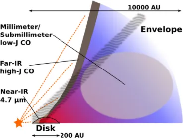
Complementary information on the CO excitation is ob-tained from near-infrared (NIR) observations of the 4.7μm fun-damental CO (v=1−0) band seen in absorption toward YSOs. Because the absorption probes a pencil beam line of sight toward the central source, the lines are more sensitive to the inner dense part of the envelope than the submillimeter emission line data, which are dominated by the outer envelope (see Fig.1). The NIR data generally reveal a cold (<30 K) and a warm (>90 K) com-ponent (Mitchell et al. 1990;Boogert et al. 2002;Brittain et al. 2005;Smith et al. 2009;Herczeg et al. 2011). The cold compo-nent is seen toward all YSOs in all of the isotopolog absorptions. However, the warm temperature varies from source to source. The question is whether the standard picture of collapse and disk formation can also reproduce these multiple temperature components.
A description of the physical models and methods is given in Sect.2. The evolution of the molecular excitation and the re-sulting far-infrared (FIR) to submm lines of the pure rotational transitions of CO is discussed in Sect.3, whereas the NIR ro-vibrational transitions is presented in Sect.4. The implication of
Disk
200 AU Near-IR
4.7 μm Far-IR high-J CO
Fig. 1.Sketch of one quadrant of an embedded protostellar system with a disk and envelope. The FIR/millimeter/submillimeter emission comes from the envelope and outflow cavity walls. On the other hand, the NIR absorption (gray shaded region) also probes the warm region close to the star through a pencil beam, illustrating the complementarity of the techniques. The dotted orange lines indicate the stellar light.
the results and whether embedded disks can be observed during Stage 0 is discussed in Sect.5. The results and conclusions are summarized in Sect.6.
2. Method
2.1. Physical structure
The two-dimensional axisymmetric model of Visser et al. (2009),Visser & Dullemond(2010) andVisser et al.(2011) was used to simulate the collapse of a rotating isothermal spheri-cal envelope into a pre-main sequence star with a circumstel-lar disk. The model is based on the analytical collapse solutions ofShu(1977, hereafter S77),Cassen & Moosman(1981, here-after CM81) andTerebey et al. (1984, hereafter TSC84). The formation and evolution of the disk follow according to theαS viscosity prescription, which includes conservation of angular momentum (Shakura & Sunyaev 1973;Lynden-Bell & Pringle 1974). The dust temperature structure (Tdust) is a key quantity for the chemical evolution, so it is calculated through full 3D continuum radiative transfer with RADMC3D1, considering the protostellar luminosity as the only heating source. The gas tem-perature is set equal to the dust temtem-perature, which has been found to be a good assumption for submm molecular lines (Doty et al. 2002;Doty et al. 2004).
The model is modified slightly in order to be consistent with observational constraints. The density atr = 1000 AU (n1000) should be at most 106 cm−3 for envelopes around low-mass YSOs (Jørgensen et al. 2002;Kristensen et al. 2012), but the in-terpolation scheme ofVisser et al.(2009) violated that criterion. To correct this, theCM81andTSC84 solutions are connected in terms of the dimension-less variableτ= Ω0tby interpolating between 100τ2and 10τ2forΩ0 =10−13Hz and between 100τ2 andτ2forΩ0=10−14Hz, whereΩ0is the envelope’s initial solid body rotation rate. The overall collapse, the structure of the disk and the chemical evolution are unaffected by this modification. The models evolve until one accretion time,tacc=M0/M˙ where 1 http://www.ita.uni-heidelberg.de/~dullemond/
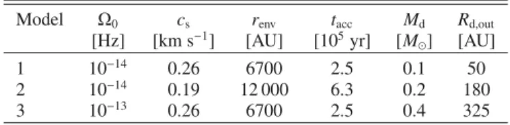
Table 1.Parameters used for the three different evolutionary models.
Model Ω0 cs renv tacc Md Rd,out [Hz] [km s−1] [AU] [105yr] [M
] [AU]
1 10−14 0.26 6700 2.5 0.1 50
2 10−14 0.19 12 000 6.3 0.2 180
3 10−13 0.26 6700 2.5 0.4 325
˙
M ∝c3
s/Gwithcs the initial effective sound speed of the enve-lope, which is tabulated in Table1.
Three different sets of initial conditions are used in this work (Table1), which are a subset of the conditions explored byVisser et al.(2009) andVisser & Dullemond(2010). Each model be-gins with a 1M envelope. The two variablesΩ0 andcs affect the final disk structure and mass. Model 1 (cs = 0.26 km s−1, Ω0=10−14Hz) produces a disk with a final mass (t/t
acc=1) of 0.1Mand a final radius of 50 AU. ChangingΩ0 to 10−13 Hz (Model 3) yields the most massive and largest of the three disks (0.4M, 325 AU). Starting with a lower sound speed of 0.19 km s−1 (Model 2) produces a disk of intermediate mass and size (0.2 M, 180 AU). The initial conditions also affect the flattened inner envelope structure. In Model 3, the flatten-ing of the inner envelope extends to>300 AU byt/tacc = 0.5 and extends up to∼1000 AU by the end of the accretion phase. In the other two models, the extent of the flattening is similar to the extent of the disk, with Model 2 showing more flatten-ing in the inner envelope than Model 1. The different evolution-ary stages are characterized by the relative masses in the diff er-ent componer-ents (Robitaille et al. 2006):Menv >> M(Stage 0,
t/tacc≤0.5),Menv<MbutMenv>Mdisk(Stage 1,t/tacc>0.5) andMenv<Mdisk(Stage 2) (see Appendix B).
Our main purpose is to investigate how the molecular lines evolve during different disk formation scenarios (Stage 0/I). Hence, the parameters were chosen to explore the formation of three different disk structures. Figure2zooms in on the final disk structures for the different models at the accretion time (t=tacc) where the red lines outline the disk surfaces. The angular ve-locities within these lines are assumed to be Keplerian while re-gions outside these lines are described by the analytical collaps-ing rotatcollaps-ing envelope solutions (Visser et al. 2009). The density structure is 2D axisymmetric with a 3D velocity field within the envelope and the disk.
2.2. CO abundance
The 12CO abundance is obtained through the adsorption and thermal desorption chemistry as described in Sect. 2.7 ofVisser et al.(2009). The main difference is that we have used both the forward and backward methods (Visser et al. 2011) to sample the trajectories through the disk and envelope. The chemistry is still solved in the forward direction.
CO completely freezes out atTd≤18 K (Visser et al. 2009). For the majority of the time steps used for the molecular line simulations, the dust temperature is well above 18 K everywhere except for the outer envelope beyond∼4000 AU. However, due to the low densities within this region, CO is still predominantly in the gas phase. Only at early time steps, early Stage 0, a large fraction of CO is frozen out within the inner envelope. Constant isotope ratios of12C/13C = 70 and16O/18O = 540 (Wilson & Rood 1994) are used throughout the model to compute the abundances of13CO and C18O.
Fig. 2.Final disk structure for the three models from Table1att = tacc. Top: gas density in the inner 500 AU. The solid line contours mark densities of 106,7,8,9 cm−3. Middle: temperature structure in the inner 500 AU. The temperature contours are logarithmically spaced from 10 to 320 K. The 20, 50 and 100 K isotherms are marked by the solid line contours.Bottom: temperature structure in the inner 200 AU. In all panels, the dotted lines illustrate the lines of sight at inclinations of 15◦, 45◦and 75◦and the red line indicates the final disk surface.
2.3. Line radiative transfer
A fast and accurate multi-dimensional molecular excitation and radiative transfer code is needed to obtain observables at a num-ber of time steps. We use the escape probability method from Bruderer et al. (2012) (based on Takahashi et al. 1983 and Bruderer et al. 2010).
The most important aspect of simulating the rotational lines is the gridding of the physical structure. There are three com-ponents in the model that require proper gridding (Fig. A.2): the outflow cavity, the envelope (>6000 AU) and the disk (<300 AU). To resolve the steep gradients between the different regions, 15 000−25 000 cells are used. A detailed description of the grid can be found in AppendixA. The line images are ren-dered at a number of time steps with a resolution of 0.1 km s−1to resolve the dynamics of the collapsing envelope and the rotating disk.
In addition to pure rotational lines in the submm and FIR, this work also explores the evolution of the NIR fundamental
The main collisional partners are p-H2 and o-H2 with the collisional rate coefficients obtained from the LAMDA database (Schöier et al. 2005;Yang et al. 2010). The dust opacities used in our model are a distribution of silicates and graphite grains covered by ice mantles (Crapsi et al. 2008). Finally, the gas-to-dust mass ratio is set to 100.
2.4. Comparing to observations
The molecular lines are simulated considering a source at a dis-tance of 140 pc. High spatial resolution in raytracing is needed for theJu ≥5 lines because of the small warm emitting region. A constant turbulent width ofb=0.8 km s−1is used in addition to the temperature and infall broadening to be consistent with the observed C18O turbulent widths toward quiescent gas surround-ing low-mass YSOs with beams>9(Jørgensen et al. 2002).
The simulated spectral cubes are convolved with Gaussian beams of 1, 9and 20with theconvolroutine in the MIRIAD data reduction package (Sault et al. 1995). The telescopes that observe the low-J rotational lines (Ju ≤ 5) typically have ≥15 beams, as does Herschel-HIFI for the higher-J lines with Ju ≈ 10. A 9 beam is appropriate for observations of
Ju >5 performed with, e.g., the ground-based APEX telescope at 650 GHz and withHerschel-PACS and HIFI for Ju > 14. A 1 beam simulates interferometric observations to be per-formed with ALMA. The submm lines are rendered nearly face-on (i ∼ 5◦) since this is the simplest geometry to quantify the disk contribution. For studies of the evolution of the velocity field, an inclination of 45◦is taken. The NIR lines are analyzed for 45◦and 75◦inclination to study the different excitation con-ditions between lines of sight through the inner envelope and the disk (Fig.2). A line of sight of 45◦probes the inner envelope and does not go through the disk while a line of sight of 75◦ grazes the top layers of the disk. Both a pencil beam approximation to-ward the center is taken as well as the full RADLite simulation to study the radiative transfer effects on those lines.
2.5. Caveats
The synthetic CO spectra were simulated without the presence of fore- and background material, such as the diffuse gas of the large-scale cloud where these YSOs are forming. The overall emission of the large-scale cloud can affect the observed line profiles within a large beam (>15), in particular theJu≤4 lines of12CO and13CO and theJ
u ≤ 2 lines of C18O. Also not in-cluded in the simulations are energetic components such as jets, shocks, UV heating and winds. These energetics strongly affect the12CO lines, especially the intensity of theJ
u ≥6 rotational transitions (Spaans et al. 1995;van Kempen et al. 2009a;Visser et al. 2012). Luminosity flares associated with episodic accre-tion events can affect the CO abundance structure as discussed inVisser & Bergin(2012). Their effect on the evolution of the CO line profile and excitation is beyond the scope of this pa-per. In general, a higher CO flux is expected during an accretion burst.
3. FIR and submm CO evolution
The FIR and submm CO lines up to the 10−9 transition (Eu = 290−304 K) have been simulated withi =5◦. The geometrical effects on the line intensities (13CO and C18O) are less than 30% for different inclinations and the derived excitation temperatures differ by less than 5%, which is smaller than the rms error on the
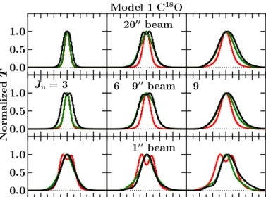
Fig. 3.Normalized C18O line profiles as functions of evolution forJ u= 3, 6 and 9 att/tacc=0.13 (red), 0.50 (green) and 0.96 (black) fori=5◦ orientation for Model 1. The lines are convolved to beams of 20(top), 9(middle) and 1(bottom).
derived temperatures. On the other hand, inclination strongly af-fects the derived moment maps and interpretation of the velocity field, therefore an inclination of 45◦is used in Sect.3.4.
3.1. Line profiles
The first time step used for the molecular line simulation is att = 1000 years (t/tacc ∼ 10−3), where the central heating is not yet turned on. The evolution of the mass and the effective temperature is shown in the AppendixB. The effective tempera-ture during this time step is 10 K and the models are still spher-ically symmetric. TheTSC84velocity profile for this time step reaches a maximum radial component of 10 km s−1 at 0.1 AU. However, CO is frozen out in the inner envelope, so the FIR and submm lines (populated up to Ju ≤ 8) show neither wing emission nor blue asymmetry as typical signposts of an infalling envelope. Instead, the CO lines probe the static outer envelope at this point, where the low density has prevented CO from freezing out.
The line profiles change shape once the effective source tem-perature increases to above a few thousand K att >104yr (see Fig.3 and AppendixBfor the line profile evolution). The line profiles become more asymmetric (Fig.B.2) toward higher ex-citation and smaller beams, because in both cases a larger con-tribution from warm, infalling gas in the inner envelope and op-tical depth affect the emission lines. The line widths are due to a combination of thermal broadening, turbulent width and ve-locity structure, but examination of models without a systematic velocity field confirm that the increase in broadening is mostly due to infall (see also Lee et al. 2004). Models 2 and 3 show narrower lines during Stage I (t/tacc ≥0.5) since they are rela-tively more rotationally dominated than in Model 1. As shown in Fig.4, the higher-J(Ju≥5) lines are broadened significantly during Stage 0.
Fig. 4.C18O 3-2 (red), 6−5 (blue) and 9−8 (black) FWHM evolution within a 9beam for the 3 different models ati=5◦orientation.
high angular resolution. A combination of CO isotopolog lines can provide a powerful diagnostic of the velocity and density structure on 10−1000 AU scales (see also Sect. 3.4).
In summary, the infalling gas can significantly broaden the optically thin gas as shown in Fig.4. The velocity profile in the inner envelope affects the broadening of the high-J (Ju > 6) line. These lines can be a powerful diagnostic of the velocity and density structure in the inner 1000 AU (≤9beams).
3.2. CO rotational temperature
The observed integrated intensities (K km s−1) are commonly an-alyzed by constructing a Boltzmann diagram and calculating the associated rotational temperature. Another useful representation is to plot the integrated flux ( Fνdν in W m−2) as a function of upper level rotational quantum number (spectral line energy distribution or SLED) to determine theJlevel at which the peak of the molecular emission occurs. The conversion between inte-grated intensities and inteinte-grated flux is given by
Fνdν= 2λk3dΩ
Tvdv. (1)
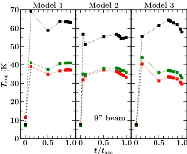
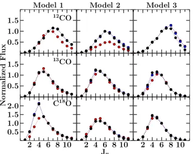
Examples of single-temperature fits through the modeled lines are shown in Fig.5for Model 1. Observationally, temperatures are generally measured fromJu = 2 to 10 (Yıldız et al. 2012, 2013) and from 4 to 10 (Goicoechea et al. 2012). The evolu-tion of the rotaevolu-tional temperatures within a 9beam is shown in Fig.6for the three models. At very early times,t/tacc <0.1, a single excitation temperature of∼8−12 K characterizes the CO Boltzmann diagrams. After the central source turns on, the exci-tation temperature is nearly constant with time. In a beam of 9, most of the flux up toJu = 10 comes from the >100 AU re-gion, which is not necessarily the>100 K gas (Yıldız et al. 2010) even for face-on orientation. Therefore, within≥9 beams, the observed emission is not sensitive to the warming up of material as the system evolves.
A value of 46 to 65 K characterizes the12CO distribution for all models. However,12CO is optically thick, which drives the temperature to higher values due to under-estimated low-J col-umn densities. The C18O and13CO distributions are fitted with similar excitation temperatures between 29 and 42 K within a 9 beam. Because Model 3 has a higher inner envelope density, the derived rotational temperature at the second time step is rela-tively high (40 K) due to an optical depth effect.
The integrated fluxes can also be used to construct CO SLEDs. The12CO SLED peaks at J
u = 6−8 with small
Fig. 5.Examples of single-temperature fits through the12CO (squares) and C18O (triangles) lines obtained from Model 1 fluxes att/t
acc=0.9 in a 9beam. The red line shows the linear fit fromJu=2 up toJu=10 while the blue line is the fit up starting fromJu =4 up toJu =10. The gray shaded regions indicate one standard deviation from the best fit.
Fig. 6. Evolution of the rotational temperature (Trot) from a single-temperature fit throughJu=2−10. The different colors are for different isotopologs:12CO (black),13CO (green) and C18O (blue). The typical errors are 15, 5 and 3 K for12CO,13CO and C18O, respectively. The different panels show the results for different models as indicated.
dependence on the heating luminosity (Fig. 7). The peak of the SLEDdoes notdepend on the beam size for beams≥9. The same applies to the 13CO and C18O SLEDs which peak at Ju = 4−5. There is no significant observable evolution in the SLEDs once the star is turned on. A passively heated sys-tem is characterized by such SLEDs regardless of the evolu-tionary state as long as the heating luminosity is ∼1−10 L (T∼1000−4500 K).
Fig. 7.Evolution of normalized CO spectral line energy distribution (SLED) in a 9beam. The CO integrated fluxes (W m−2) are normal-ized toJu=6. The different colors indicate different times:t/tacc∼0.50 (red), 0.75 (blue), 0.96 (black).
rotational temperatures are∼40−50 K. There is less spread than within the 9 beam due to the higher densities bringing the ex-citation closer to LTE. Without a significant disk contribution in a 1beam (Model 1), the13CO excitation temperature is closer to 60 K while that of C18O is similar to the other models at ∼40 K. The12CO rotational temperature isT
rot70 K in all of the models. Furthermore, the CO SLED within a 1beam peaks atJu =6,8 and 10 for C18O,13CO and12CO, respectively.
A comparison with the sample presented in Yıldız et al. (2013) indicates that the lack ofTrotevolution is consistent with observations, and our predicted values forTrotmatch the data. On the other hand, the observed13COTrotand SLED are gener-ally higher than predicted, which suggests an additional heating component is needed to excite the13CO lines. A more detailed comparison between model prediction and observation can be found inYıldız et al.(2013).
In summary, both rotational temperatures derived from Boltzmann diagrams and CO SLEDs of passively heated sys-tems do not evolve with time once the star is turned on. Optically thin13CO and C18O lines are characterized by single excitation temperatures of the order 30−40 K within a wide range of beams (≥9). The CO SLED peaks atJu=7±1 andJu=4−5 for12CO and other isotopologs, respectively. In 1beam, the peak of the SLED shifts upward by∼2Jlevels and a warmer rotational tem-perature by 10 K in the presence of a disk.
3.3. Disk contribution to line fluxes
After deriving a number of observables, an important question is, what the fraction of the flux contributed by the disk is? This contribution can be calculated from the averaged (over line pro-file and direction) escape probability of the line emissionηul, which is the probability that a photon escapes both the dust and line absorption (Takahashi et al. 1983;Bruderer et al. 2012). The escape probabilities are used to calculate the cooling rate, Γcool,ν, of each computational cell and each transition with the
following formula Γcool,ν= V
4πhνulAulnxuηul, (2)
Fig. 8. Disk contribution as a function of Ju within 1 (140 AU at 140 pc) for the three different models. The different colors correspond to different evolutionary stages:t/tacc∼0.50 (red,Menv/Mdisk≥3), 0.75 (blue,Menv/Mdisk∼1), 0.96 (black,Menv/Mdisk<1).
whereνulis the frequency of the line,Aulis the EinsteinA coef-ficient,xuis the normalized population level andnis the density of the molecule. The disk contribution is then the ratio of the sum of cooling rates from the cells in the disk compared to the cells within a Gaussian beam. The cooling rates are weighted with a Gaussian beam of size 9or 1 while the disk emitting region is defined as shown in Fig.2. The flux is then given through an integration of line of sight,Fν= Γcool,νdsLOS, which translates into the same constant factor in both disk and total fluxes.
For a single-dish 9 beam, one needs to go to higher rota-tional transitions withJu > 6 at later stages to obtain a>50% disk contribution, if the disk can be detected at all (Fig.B.5). The disk is difficult to observe directly in12CO and13CO emis-sion since the lines quickly become optically thick unless lines withJu >10 are observed. A larger disk contribution is seen in the optically thin C18O lines, but here the low absolute flux may become prohibitive.
For example, the expected C18O disk fluxes for Ju > 14 within the PACS wavelength range are ≤10−20 W m−2 which will take >100 h to detect with PACS. Herschel-HIFI is able to spectrally resolved the C18O J
u = 10 and 9 lines but has a∼20 beam, which lowers the disk fraction by a factor of 2 relative to a 9beam. Peak temperatures of only 1−8 mK dur-ing Stage 0 and 2−12 mK in Stage I phase are expected, which are readily overwhelmed by the envelope emission. The spec-trally resolved C18O spectra observed with HIFI indeed do not show any sign of disk emission, consistent with our predictions (San Jose-Garcia et al. 2013;Yıldız et al. 2012,2013).
A more interesting result is the disk contribution to the CO lines within a 1 (140 AU) region as shown in Fig. 8. The simulations suggest a significant disk contribution (>50%) for the 13CO and C18O lines within this scale, even for the
Fig. 9.13CO and C18O zeroth (left panels) and first (right panels) moment maps for Model 1 and 3 at 45◦inclination at a resolution of 1. The red
arrows indicate the direction of infall and rotationally supported disk. The velocity scale is given on theright-hand side of the left figure.
envelope within 1att/tacc=0.5. Thus, the relatively more op-tically thin CO isotopolog emission is dominated by the central rotating disk starting from the Stage 1 phase (t/tacc≥0.5).
3.4. Disentangling the velocity field
How can the rotating and infalling flattened envelope be disen-tangled from the Keplerian motion of the disk? The evolution of the rotationally dominated region is consistent with that reported byBrinch et al.(2008) based on more detailed hydrodynamics simulations. All models become rotationally dominated within 500 AU att/tacc>0.3.
The presence of an embedded disk can be inferred from the presence of elongated13CO and C18O integrated intensity maps (moment 0 of Fig.9) coupled with the moment 1 map. In the presence of a stable disk, the zeroth moment map is elongated perpendicular to the outflow axis with a double peaked structure. This feature is not seen in Model 1 (Fig.9 left) since the disk is much smaller than the 1 beam. In the case of Model 3, the relatively massive disk exhibits a double peaked zeroth moment map which is perpendicular to the outflow direction.
A velocity gradient is seen in the moment 1 maps for both Models 1 and 3. With the high resolution of the modeled spec-tra, it is possible to differentiate between the disk and envelope (Hogerheijde 2001). The presence of a velocity gradient along the major axis of the elongation in the moment 1 map is a clear sign of a stable embedded disk in the case of Model 3. In addi-tion, from the analysis in Sect.3.3, we can also attribute the bulk of optically thin emission in Model 3 to the disk. Meanwhile, the infalling rotating envelope contribution can be detected through the fact that the moment 1 map is not perfectly aligned but skewed. On the other hand, a velocity gradient without the pres-ence of elongation in the zeroth moment map such as in Model 1 (Fig.9) indicates an infalling envelope.
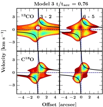
Position–velocity (PV) diagrams provide another way to study the velocity structure. Figure10shows PV slices follow-ing the direction of the major axis of the disk (PA=90◦) in the integrated intensity map in the 3−2 and 6−5 lines. A sim-ple way to analyze PV diagrams is to separate the diagram into four quadrants and examine which quadrants have considerable
Fig. 10.Position–velocity slice for the13CO and C18OJ
u=3 andJu=6 transitions along the major axis of the zeroth moment map. The solid black lines are the Keplerian velocity structure calculated from the stel-lar mass.
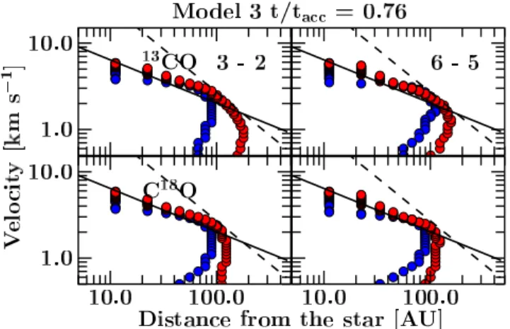
Fig. 11.Velocity as function of distance of the peak intensity position from the protostar, as measured in each channel map and for the same transitions as in Fig.10. The red and blue colors represent the red- and blue-shifted components. The solid black line indicates the expected Keplerian structure from the stellar mass in the model, where as the dashed lines indicate thev∝R−1relation as a comparison.
Focusing on Model 3 att/tacc=0.76 (near the end of Stage I) as shown in Fig.10, the C18O PV diagrams show a clearer pure rotation dominated structure than the13CO lines. They can thus be used to constrain the stellar mass as long as the inclination is known. Also, the higher-Jlines provide a better view into the ro-tating structure and should give tighter constraints on the stellar mass.
Another method is to plot the velocity as function of dis-tance of the position of the peak intensity (Sargent & Beckwith 1987). This is done for the red-shifted and blue-shifted compo-nents, plotted in Fig.11. The method is similar to the spectroas-trometry technique employed in the optical and NIR observa-tions (Takami et al. 2001;Baines et al. 2006;Pontoppidan et al. 2008). A Keplerian disk is characterized by av∝r−0.5with large contribution from the high velocity gas which is optically thin. As noted bySargent & Beckwith(1987), as long as the line is spectrally resolved (dV =0.1 km s−1), the peak position corre-sponds to the maximum radius of a given velocity. On the other hand, the emission at low velocities (dV∼V) is relatively more optically thick and is dominated by the infalling rotating enve-lope which peaks closer to the center (no offset). Such an anal-ysis can be performed directly from the interferometric data and is a powerful tool in searching for embedded rotationally stable disks out of the rotating infalling envelope.
Why is there a difference between the red-shifted and blue-shifted components in Fig. 11? At high velocities, this is due to unresolved emission hence the different velocity components simply peak at the same position and the difference reflects the uncertainty in locating the emitting region. At low velocities, the optically thick infalling rotating envelope affects the peak positions. In an infalling envelope, the blue-shifted emission is relatively more optically thin than the red-shifted emission (Evans 1999). Such difference in the optical depth causes the red- and blue-shifted emissions to be asymmetric as found in the moment 1 map.
4. NIR CO absorption lines
A complementary probe of the molecular excitation conditions is provided by the NIR CO ro-vibrational absorption lines. In this work, we concentrate on thev=1−0 band at 4.76μm. This
absorption takes place along the line of sight through the enve-lope and/or disk up to where the continuum is formed. The ab-sorption lines are therefore computed for different inclinations of 45◦ and 75◦. The inclinations were chosen such that they probe the envelope (>15◦) and the part of the disk that is not completely optically thick such that there is enough observable NIR continuum (≤75◦), i.e., lines of sight that graze the disk at-mosphere. Since our focus is on the excitation, the absorption lines have been calculated without any velocity field besides a turbulent width (Dopplerb) of 0.8 km s−1. More importantly, the formation of the 4.7μm continuum is strongly dependent on the inclination which affect the molecular absorption lines.
4.1. Evolution of NIR absorption spectra
4.1.1. Radiative transfer and non-LTE effects
The line center optical depth is one of the quantities derived from the model that can be compared to observations. This optical depth can either be determined by computing the line of sight integrated column densities and converting this to optical depth or by using a full RADLite calculation. For both approaches, the same level populations are used, i.e., the same model for the CO excitation is adopted as in Sect. 3. In the simplest method, the line center optical depth is obtained from
τ0=
c3g u
8π√πbν3g l
AulNl, (3)
whereνis the line frequency andNlis the lower level column density along the line of sight. The main difference between the methods is that RADLite solves the radiative transfer equation along the line of sight and thus accounts for continuum and line optical depth effects and scattered continuum photons, while such effects are not considered in the column density approach. In addition, RADLite accounts for the continuum formation, while a ray through the center does not. Thus, the two meth-ods effectively compare the total mass present along a ray and the observed mass as probed by the line optical depth returned by RADLite. The optical depth is extracted from the RADLite spectra using the line-to-continuum ratio at the line center.
As discussed and illustrated extensively in Appendix C.1, the two approaches can give very different results, especially for the higher J lines for which the line optical depths can differ by more than an order of magnitude. The main reason is illus-trated in Fig.C.3, which shows the region where the NIR contin-uum arises. For small inclinations, the contincontin-uum is essentially point-like, but for higher inclinations larger radii contribute sig-nificantly and the continuum is no longer a point source. Thus, for high inclinations, the high-Jlines start absorbing off-center, away from warm gas in the inner few AU that are included in the column method. The location of the continuum is typically at>10 AU ati=75◦which results in two to three orders of mag-nitude difference in total column density. For the case ofi∼45◦, the result depends on the physical structure in the inner few AU but the absorption can miss the warm high density region close to the midplane of the disk where most of theJ≥10 is located (Fig.C.2).
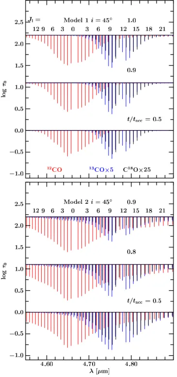
Fig. 12.Evolution of the12CO (red),13CO (blue) and C18O (black) ab-sorption lines for Model 1 ati=45◦. The evolution of the absorption lines for Model 2 is shown at thebottom panel. The lower rotational levels are indicated on top of the first spectrum. All of the13CO lines are multiplied by 5 and C18O lines by 25.
4.1.2. NIR spectra
The NIR absorptions are rendered with RADLite fort/tacc≥0.5 which starts when Menv ∼ M (Stage 0/I boundary) in or-der to have a strong 4.7μm continuum. Figure12 show the P and R branches of the CO isotopologs for Model 1 and 2 which show the greatest difference. In general, as shown in Fig. 12, the higher-Jabsorptions are stronger as the system evolves into Stage II due to the central luminosity. For Model 1, att/tacc = 0.5, the 12CO absorptions can be seen up to J = 16, and up
toJ = 9 for13CO and 7 for C18O. The number of absorption lines that are aboveτν = 3×10⁻³(the 3σobservational limit
with instruments such as VLT-CRIRES) doubles at the end of the accretion phase and the highest observableJshifts from 16 to>30 for12CO and up to∼15−20 for the isotopologs.
At early times, a similar number of lines are found for Model 3 but their optical depths are lower due to the difference in the inner envelope structure. On the other hand, the number of lines in Model 2 is much higher than in the other two mod-els due to the lower continuum optical depth in the inner enve-lope. Thus, the absorbing column starts deeper than in the other two models, which results in stronger absorption features and an increased number of detectable high-Jlines, up toJ > 40 for 12CO,J∼25 for13CO andJ∼15 for C18O (Fig.12). Thus, in principle the appearance of the NIR spectrum could be a sensi-tive probe of the inner envelope structure. In practice, the12CO absorption will be affected by outflows and winds so the13CO and C18O isotopologs are most useful for this purpose.
4.2. Rotational temperatures
A directly related observable is the rotational temperature de-rived from a Boltzmann diagram. Thus, the RADLite NIR spec-tra need to be converted into column densities. For this conver-sion, we use a standard curve-of-growth analysis (Spitzer 1989) withb = 0.8 km s−1 and oscillator strengths derived from the EinsteinAulcoefficients. By using the curve-of-growth method, it is assumed that the spectral lines are unresolved.
An example of a Boltzmann diagram is shown in Fig.C.1 together with a two-temperature fit, as commonly done in obser-vations (Mitchell et al. 1990;Smith et al. 2009;Herczeg et al. 2011). The rotational temperature of the cold component is ob-tained from fitting the P(1) to P(4) lines (El < 40 K). Lines higher than P(5) (El >40 K) are used to obtain the temperature of the warm component. Model 2 att/tacc=0.78 is used since it clearly shows the break between the two temperatures.
How do the two temperatures evolve with time? As Table2 shows, the cold component is between 20 and 35 K with no significant evolution, except in Model 2, as the disk is build-ing up. The warm component, however, increases with inclina-tion and time. The derived warm temperature component ranges from<100 up to∼520 K and traces the warming up of material in the inner region as the envelope dissipates. From the simula-tions, a>400 K warm component is a signature of an evolved system.
Table 2.NIR rotational temperatures derived fromτ0>10−3lines fori=45◦and 75◦.
12CO 13CO C18O
t/tacc i Tcold Twarm Tcold Twarm Tcold Twarm
[◦] [K] [K] [K] [K] [K] [K]
Model 1
0.50 45 21±9 80±9 18±11 49±18 19±13 ... 75 20±9 66±8 17±10 44±10 18±10 ... 0.76 45 26±10 142±21 19±11 72±20 19±14 ... 75 25±12 260±67 25±12 273±69 19±13 ... 0.96 45 28±10 201±36 28±13 207±46 21±16 ... 75 25±10 271±61 25±13 301±80 20±13 ...
Model 2
0.50 45 34±20 245±61 34±25 253±61 29±23 183±51 75 31±20 293±85 31±20 302±86 27±19 209±67 0.78 45 31±20 327±100 31±20 340±110 28±19 264±89 75 20±11 489±210 19±11 481±192 18±11 423±230 0.94 45 28±18 402±156 28±18 410±152 26±17 333±139 75 18±11 544±255 17±10 527±223 17±10 495±308
Model 3
0.50 45 21±6 193±37 16±8 42±21 19±9 ...
75 16±7 37±7 16±10 ... 16±11 ...
0.76 45 23±9 287±80 22±9 304±85 17±11 ... 75 22±8 289±81 21±8 302±83 17±10 ... 0.96 45 22±9 366±128 21±8 381±129 17±10 ... 75 18±8 361±121 18±7 371±119 16±9 ...
Fig. 13.Integrated gas column density along the different viewing an-gles for Model 2. The red and blues lines indicate the warm (T>100 K) and cold gas (T <50 K), respectively. The approximate continuum op-tical depths,τc=1 and 10, are also shown to indicate the amount ma-terial that is missed by properly solving the radiative transfer equation.
continuum optical depth, higher warm temperatures can be ob-served as the absorption probes deeper to smaller radii than the other two models.
5. Discussion
We have presented the evolution of CO molecular lines based on the standard picture of a prestellar core collapsing to form a star and 2D circumstellar disk. The main aim of this work is to study the evolution of observables that are derived from the spectra such as rotational temperatures, line profiles, and veloc-ity fields. Specifically, signatures of disk formation during the embedded stage that can be obtained with the most commonly used molecule, CO, are investigated.
5.1. Detecting disk signatures in the embedded phase
How can one determine whether disks have formed in the ear-liest Stage 0? As discussed in Sect. 3.3, it is difficult to iso-late an embedded disk component in single-dish observations. The disk contribution to the observed flux within>9beams is only significant (>60%) for the13CO and C18OJ
u >9 lines at
t/tacc>0.75. However, the absolute fluxes are too low to be de-tected. Thus, spatially resolved observations at sub-arcsec scale are needed.
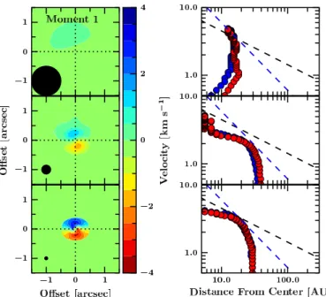
What are the signatures of an embedded rotationally sup-ported disk on subarcsecond scales? We have analyzed some of the simulated images during the Stage 0 phase at a resolu-tion of 0.1as can readily be observed with ALMA. Figure14 shows the C18O 3−2 moment-one map during the Stage 0 phase of Model 1 with a disk extending up to 20 AU at a resolution of 1, 0.3 and 0.1. Velocity gradients are present in all of the moment-one maps although it is weaker within a 1beam. The right panel of the figure shows the spectroastrometry (Fig.11) within the different resolutions. The velocity gradient within a 0.5−1beam exhibits av∝R−1relation since the inner envelope dominates the emission. Within the smaller beams, the velocity gradient is resolved into two components:v∝R−1(blue dashed line) due to envelope andv∝R−0.5(black dashed line) due to the stable disk. Av∝R−0.5can be seen when the disk is marginally resolved, however, the derived stellar mass is far below the real stellar mass. It is very important that the disk is fully resolved in order to derive the stellar mass. With the C18O lines, a resolved embedded disk in Stage 0 would have the following features:
– Elongated moment-zero map.
– A transition between an infalling envelope to a rotating disk: a skewed moment-one map.
– The Keplerian structure exhibits a clear v ∝ R−0.5 (Fig.11 and bottom of Fig.14) velocity gradient perpendicular to the outflow.
Fig. 14.C18O 3−2 moment-one (left) and spectroastrometry (right) for Model 1 at the end of Stage 0 convolved to a 1 (top), 0.3(middle) and 0.1(bottom) as shown by the solid circle. The Keplerian structure at this stage extends up to 20 AU (0.14radius). The black dashed line in the right panel shows thev∝R−0.5and the blue dashed line indicates thev∝R−1relation.
array in less than 30 min for the C18O 2−1 transition or up to 4 hours for the 6−5 transition. For Models 2 and 3, the disks have grown up to∼50 AU near the end of Stage 0 and up to twice more massive, thus it will take less than 2 h to observe them with ALMA in the 6−5 transition and less than 30 min in the 2−1 and 3−2 transitions. Therefore, ALMA will allow us, for the first time, to test whether rotationally supported disks have grown beyond 10 AU by the end of the Stage 0 phase.
The question of when rotationally supported disks form is crucial to the physical and chemical evolution of accretion disks. In our evolutionary models, the disks have radii up to 50 AU at the end of Stage 0 phase and can be as small as 20 AU.Dapp & Basu(2010) andDapp et al.(2012) numerically showed that disks do not grow beyond 10 AU during the Stage 0 phase in the presence of magnetic fields due to the magnetic breaking prob-lem (see alsoLi et al. 2011;Joos et al. 2012). This is consistent with the lack of observed rotationally supported disks toward Stage 0 objects so far (Brinch et al. 2009;Maury et al. 2010). On the other hand, there is a growing body of observational evidence for rotating disks in Stage I YSOs (Brinch et al. 2007;Lommen et al. 2008;Jørgensen et al. 2009;Takakuwa et al. 2012). The size of the rotationally supported disk depends on the initial pa-rameters of the collapsing envelope. In our models, the sizes of Models 2 and 3 are consistent with the observed Keplerian ve-locity structure in Stage I sources (Jørgensen et al. 2009).
An additional caveat is that our models lead to a Keplerian disk with a flattened inner envelope on similar scales as the stable disk. Hydrodynamical simulations, on the other hand, show a stable disk embedded in a much larger rotating flattened structure and with more turbulent structure (Brinch et al. 2008; Kratter et al. 2010). Furthermore, the 3D simulations byHarsono et al. (2011) suggest that 50% of the embedded disk is sub-Keplerian due to interaction with the envelope. The predicted moment 1 maps and spectroastrometry with the current models
should be performed for these numerical simulations for com-parison with ALMA observations.
5.2. Probing the temperature structure
The derived rotational temperatures from the submm and FIR lines (Ju=1−10) within>9beams do not evolve with time, in contrast with the continuum SED, and largely trace the outer envelope (Sect.3.2). Even though the disk structure is hotter with time, the emission that comes from within that region is much smaller than the beam. The mass weighted temperature of the system which contributes to the overall emission is constant with time. The rotational temperatures also cannot diff erenti-ate between the three different evolutionary models. In addition, the peak of the CO SLED is constant throughout the evolution atJu =4 for the13CO and C18O. The higher observed excita-tion temperatures for12CO and13CO in a wide range of low-mass protostars from submm and FIR data point to other physi-cal processes that are present in the system such as UV heating and C-shock components that affect theJ≥5 lines (Visser et al. 2012;Yıldız et al. 2012).
The NIR absorption lines toward embedded YSOs are com-plementary to the submm/FIR rotational lines. Both techniques probe the bulk of the cold envelope, but the NIR lines also probe the warm component because the lines start absorbing at the
τ∼1 surface deep inside the inner envelope. Consequently, the cold component present in the NIR lines should be similar to the component observed in the submm. Indeed, the typical ro-tational temperatures of 20−30 K found in the NIR models for C18O are comparable to the values of 30−40 K found from the submm simulations.
The warm up process is accessible through NIR molecular absorption lines. In Sect.4.2, it is found that the warm compo-nent of the Boltzmann diagram evolves with time. The derived warm temperatures have a large spread depending on inclination and density structure in the inner few AU. A higher inner enve-lope and disk density correspond to a∼100 K warm component, whereas a more diffuse inner envelope has a warmer tempera-ture that can be up to 500−600 K. Thus, as long as the incli-nation is known, the temperature of the warm component may give us a clue on the density structure of the inner few AU where the>100 K gas resides.
The predicted cold and warm temperatures can be compared with those found in NIR data toward Stage I low-mass YSOs. For the cold component, a temperature of 15 K has been found for L1489 from13CO data (Boogert et al. 2002), and 10−20 K for Reipurth 50, Oph IRS43 and Oph IRS 63 from13CO and C18O data (Smith et al. 2009;Smith et al. 2010), consistent with our envelope models. For the warm component, values ranging from 100 to 250 K are found for these sources from the iso-topolog data. These warm rotational temperatures are on the low side of the model values in Table2 for the later evolutionary stages, and may indicate either a compact envelope (high in-ner envelope densities) and/or high inclination (which effectively limits the absorption lines to probe the inner envelope compo-nent). Independent information on the inclination is needed to further test the physical structure of those sources.
6. Summary and conclusions
non-LTE molecular excitation has been computed with an es-cape probability method and spectral cubes have been simu-lated for both the FIR and NIR regimes. The gas temperature is taken to be well coupled to the dust temperature as obtained through a continuum full radiative transfer code. With the avail-ability of spectrally resolved data from single dish submillimeter telescopes, theHerschelSpace Observatory, VLT CRIRES, and ALMA, it is now possible to compare the predicted collapse dy-namics with observations. We have focused the analysis on the 13CO and the C18O lines since12CO lines are dominated by out-flows and UV heating. The main conclusions are as follows:
– Spectrally resolved molecular lines are important in compar-ing theoretical models of star formation with observations and to distinguish the different physical components. The collapsing rotating envelope can readily be studied through the C18O lines. Their FWHM probes the collapse dynamics, especially for the higher-J(Ju≥6) lines where up to 50% of the line broadening can be due to infall.
– The derived rotational temperatures and SLED from submm and FIR pure rotational lines are found to be independent of evolution and do not probe the warm up process, in contrast to the continuum SED. The predicted rotational temperatures are consistent with observations for C18O for a large sample of low-mass protostars.
– The predicted12CO and 13CO rotational temperatures and high-Jfluxes are lower than those found in observations of a wide variety of low-mass sources (Goicoechea et al. 2012; Yıldız et al. 2012,2013). This indicates the presence of ad-ditional physical processes that heat the gas such as shocks and UV heating of the cavity walls (Visser et al. 2012). – The NIR absorption lines are complementary to the
FIR/submm lines since they probe both the cold outer en-velope and the warm up process. Values obtained for the cold component are consistent with the observational data and models. For the warm component, the observed values are generally on the low side compared with the model re-sults. The high-JNIR lines are strongly affected by radiative transfer effects, which depend on the physical structure of the inner few AU and thus form a unique probe of that region. – The simulations indicate that an embedded disk in both
Stage 0 (Menv > M) and I (Menv < Mbut Mdisk < Menv) does not contribute significantly (<50%) to the emergent
Ju < 8 lines within>9 beams. Higher-Jisotopolog lines have a higher contribution but are generally too weak to ob-serve. The disk contribution is significantly higher within 1beam and the evolution within such a beam indicate rota-tionally supported disks should be detectable in Stage I phase consistent with observations (Jørgensen et al. 2009). – Embedded disks during the Stage I phase are generally
large enough to be detected with current interferometric in-struments with 1 resolution, consistent with observations. On the other hand, high signal-to-noise ALMA data at ∼0.1 resolution are needed in order to find signatures of embedded disks during the Stage 0 phase. A careful analysis is needed to disentangle the disk from the envelope. – We have shown that the rotationally dominated disk can be
disentangled from the collapsing rotating envelope with high signal-to-noise and high spectral resolution interferometric observations (Sect.3.4). The spectroastrometry with ALMA by plotting the velocity as function of peak positions can re-veal the size of the Keplerian disk. The13CO lines within in-terferometric observations may still be contaminated by the
infalling rotating envelope. Thus, more optically thin tracers are required.
The three different collapse models studied here differ mostly in their physical structure and velocity fields on 10−500 AU scales and illustrate the range of values that are likely to be encoun-tered in observational studies of embedded YSOs. It is clear that the combination of spatially and spectrally resolved molecular line observations by ALMA and at NIR are crucial in determin-ing the dynamical processes in the innermost regions durdetermin-ing the early stages of star formation. A comparison between the stan-dard picture presented here or hydrodynamical simulations and molecular line observations of Stage 0 YSOs will further test the theoretical picture of star and planet formation.
Acknowledgements. We would like to thank Steve Doty for stimulating dis-cussions on continuum and line radiative transfer and for allowing us to use his chemistry code. We are also grateful to Kees Dullemond for providing RADMC (and RADMC3D) and to Klaus Pontoppidan for RADLite. We thank the anonymous referee for the constructive comments, which have im-proved this paper. This work is supported by the Netherlands Research School for Astronomy (NOVA) and by the Space Research Organization Netherlands (SRON). Astrochemistry in Leiden is supported by the Netherlands Research School for Astronomy (NOVA), by a Spinoza grant and grant 614.001.008 from the Netherlands Organisation for Scientific Research (NWO), and by the European Community’s Seventh Framework Programme FP7/20072013 under grant agreement 238258 (LASSIE).
References
Aikawa, Y., Wakelam, V., Garrod, R. T., & Herbst, E. 2008, ApJ, 674, 984 Baines, D., Oudmaijer, R. D., Porter, J. M., & Pozzo, M. 2006, MNRAS, 367,
737
Belloche, A., André, P., Despois, D., & Blinder, S. 2002, A&A, 393, 927 Boogert, A. C. A., Hogerheijde, M. R., & Blake, G. A. 2002, ApJ, 568, 761 Brinch, C., Crapsi, A., Jørgensen, J. K., Hogerheijde, M. R., & Hill, T. 2007,
A&A, 475, 915
Brinch, C., Hogerheijde, M. R., & Richling, S. 2008, A&A, 489, 607 Brinch, C., Jørgensen, J. K., & Hogerheijde, M. R. 2009, A&A, 502, 199 Brittain, S. D., Rettig, T. W., Simon, T., & Kulesa, C. 2005, ApJ, 626, 283 Brown, D. W., Chandler, C. J., Carlstrom, J. E., et al. 2000, MNRAS, 319, 154 Bruderer, S., Benz, A. O., Stäuber, P., & Doty, S. D. 2010, ApJ, 720, 1432 Bruderer, S., van Dishoeck, E. F., Doty, S. D., & Herczeg, G. J. 2012, A&A,
541, A91
Cassen, P., & Moosman, A. 1981, Icarus, 48, 353
Chiang, H.-F., Looney, L. W. K. T., Mundy, L. G., & Mouschovias, T. C. 2008, ApJ, 680, 474
Crapsi, A., Devries, C. H., Huard, T. L., et al. 2005, A&A, 439, 1023
Crapsi, A., van Dishoeck, E., Hogerheijde, M. R., Pontoppidan, K., & Dullemond, C. 2008, A&A, 486, 245
Dapp, W. B., & Basu, S. 2010, A&A, 521, L56
Dapp, W. B., Basu, S., & Kunz, M. W. 2012, A&A, 541, A35 de Graauw, T., Helmich, F. P., Phillips, T. G., et al. 2010, A&A, 518, L6 Doty, S. D., van Dishoeck, E. F., van der Tak, F. F. S., & Boonman, A. M. S.
2002, A&A, 389, 446
Doty, S. D., Schöier, F. L., & van Dishoeck, E. F. 2004, A&A, 418, 1021 Dunham, M. M., Evans, N. J., Terebey, S., Dullemond, C. P., & Young, C. H.
2010, ApJ, 710, 470
Enoch, M. L., Corder, S., Dunham, M. M., & Duchêne, G. 2009, ApJ, 707, 103 Evans, II, N. J. 1999, ARA&A, 37, 311
Evans, II, N. J., Lee, J.-E., Rawlings, J. M. C., & Choi, M. 2005, ApJ, 626, 919 Goicoechea, J. R., Cernicharo, J., Karska, A., et al. 2012, A&A, 548, A77 Griffin, M. J., Abergel, A., Abreu, A., et al. 2010, A&A, 518, L3 Harsono, D., Alexander, R. D., & Levin, Y. 2011, MNRAS, 413, 423 Hayashi, M., Ohashi, N., & Miyama, S. M. 1993, ApJ, 418, L71
Herczeg, G. J., Brown, J. M., van Dishoeck, E. F., & Pontoppidan, K. M. 2011, A&A, 533, 112
Herczeg, G. J., Karska, A., Bruderer, S., et al. 2012, A&A, 540, A84 Hogerheijde, M. R. 2001, ApJ, 553, 618
Hogerheijde, M. R., & Sandell, G. 2000, ApJ, 534, 880
Hogerheijde, M. R., van Dishoeck, E. F., Blake, G. A., & van Langevelde, H. J. 1998, ApJ, 502, 315
Joos, M., Hennebelle, P., & Ciardi, A. 2012, A&A, 543, A128
Jørgensen, J. K., Bourke, T. L., Myers, P. C., et al. 2009, A&A, 507, 861 Keene, J., & Masson, C. R. 1990, ApJ, 355, 635
Kratter, K. M., Matzner, C. D., Krumholz, M. R., & Klein, R. I. 2010, ApJ, 708, 1585
Kristensen, L. E., van Dishoeck, E. F., Bergin, E. A., et al. 2012, A&A, 542, 8 Lee, J.-E., Bergin, E. A., & Evans, N. J. 2004, ApJ, 617, 360
Lee, J.-E., Evans, N. J., & Bergin, E. A. 2005, ApJ, 631, 351 Li, Z.-Y., Krasnopolsky, R., & Shang, H. 2011, ApJ, 738, 180
Lommen, D., Jørgensen, J. K., van Dishoeck, E. F., & Crapsi, A. 2008, A&A, 481, 141
Lynden-Bell, D., & Pringle, J. E. 1974, MNRAS, 168, 603 Manoj, P., Watson, D. M., Neufeld, D. A., et al. 2013, ApJ, 763, 83 Maury, A. J., André, P., Hennebelle, P., et al. 2010, A&A, 512, 40
Mitchell, G. F., Maillard, J.-P., Allen, M., Beer, R., & Belcourt, K. 1990, ApJ, 363, 554
Ohashi, N., Hayashi, M., Ho, P. T. P., et al. 1997, ApJ, 488, 317 Poglitsch, A., Waelkens, C., Geis, N., et al. 2010, A&A, 518, L2
Pontoppidan, K. M., Blake, G. A., van Dishoeck, E. F., et al. 2008, ApJ, 684, 1323
Pontoppidan, K. M., Meijerink, R., Dullemond, C. P., & Blake, G. A. 2009, ApJ, 704, 1482
Robitaille, T. P., Whitney, B. A., Indebetouw, R., Wood, K., & Denzmore, P. 2006, ApJS, 167, 256
Robitaille, T. P., Whitney, B. A., Indebetouw, R., & Wood, K. 2007, ApJ, 169, 328
Rothman, L. S., Jacquemart, D., Barbe, A., et al. 2005, J. Quant. Spectr. Rad. Transf., 96, 139
Saito, M., Kawabe, R., Kitamura, Y., & Sunada, K. 1996, ApJ, 473, 464 San Jose-Garcia, I., Mottram, J. C., Kristensen, L. E., et al. 2013, A&A, 553,
A125
Sargent, A. I., & Beckwith, S. 1987, ApJ, 323, 294
Sault, R. J., Teuben, P. J., & Wright, M. C. 1995, Astronomical Data Analysis Software and Systems IV, 77, 433
Schöier, F. L., van der Tak, F. F. S., van Dishoeck, E. F., & Black, J. H. 2005, A& A, 432, 369
Shakura, N. I., & Sunyaev, R. A. 1973, A&A, 24, 337 Shu, F. H. 1977, ApJ, 214, 488
Smith, R. L., Pontoppidan, K. M., Young, E. D., Morris, M. R., & van Dishoeck, E. F. 2009, ApJ, 701, 163
Smith, R. L., Pontoppidan, K. M., Young, E. D., & Morris, M. R. 2010, in Lunar and Planetary Inst. Technical Report, Lunar and Planetary Institute Science Conference Abstracts, 41, 2254
Spaans, M., Hogerheijde, M. R., Mundy, L. G., & van Dishoeck, E. F. 1995, ApJ, 455, L167
Spitzer, L., Jr. 1989, ARA&A, 27, 1
Takahashi, T., Silk, T., & Holenbach, D. J. 1983, ApJ, 275, 145 Takakuwa, S., Saito, M., Lim, J., et al. 2012, ApJ, 754, 52
Takami, M., Bailey, J., Gledhill, T. M., Chrysostomou, A., & Hough, J. H. 2001, MNRAS, 323, 177
Terebey, S., Shu, F. H., & Cassen, P. 1984, ApJ, 286, 529 Tobin, J. J., Hartmann, L., Chiang, H.-F., et al. 2011, ApJ, 740, 42 Tobin, J. J., Hartmann, L., Chiang, H.-F., et al. 2012, Nature, 492, 83
van Kempen, T. A., van Dishoeck, E. F., Güsten, R., et al. 2009a, A&A, 501, 633
van Kempen, T. A., van Dishoeck, E. F., Güsten, R., et al. 2009b, A&A, 507, 1425
van Kempen, T. A., van Dishoeck, E. F., Salter, D. M., et al. 2009c, A&A, 498, 167
van Kempen, T. A., Kristensen, L. E., Herczeg, G. J., et al. 2010, A&A, 518, A121
van Weeren, R. J., Brinch, C., & Hogerheijde, M. R. 2009, A&A, 497, 773 Visser, R., & Bergin, E. A. 2012, ApJ, 754, L18
Visser, R., & Dullemond, C. P. 2010, A&A, 519, A28
Visser, R., van Dishoeck, E. . F., Doty, S., & Dullemond, C. P. 2009, A&A, 495, 881
Visser, R., Doty, S. D., & van Dishoeck, E. F. 2011, A&A, 534, A132 Visser, R., Kristensen, L. E., Bruderer, S., et al. 2012, A&A, 537, A55 Whitney, B. A., Wood, K., Bjorkman, J. E., & Wolff, M. J. 2003, ApJ, 598, 1079 Wilson, T. L., & Rood, R. 1994, ARA&A, 32, 191
Yang, B., Stancil, P. C., Balakrishnan, N., & Forrey, R. C. 2010, ApJ, 718, 1062 Yıldız, U. A., van Dishoeck, E. F., Kristensen, L. E., et al. 2010, A&A, 521, L40 Yıldız, U. A., Kristensen, L. E., van Dishoeck, E. F., et al. 2012, A&A, 542, A86 Yıldız, U., Kristensen, L., van Dishoeck, E., et al. 2013, A&A, in press,
DOI:10.1051/0004-6361/201220849 Young, C. H., & Evans, N. J. 2005, ApJ, 627, 293
Young, C. H., Jørgensen, J. K., Shirley, Y. L., et al. 2004, ApJS, 154, 396 Zhou, S., Evans, N. J., Kömpe, C., & Walmsley, C. M. 1993, ApJ, 404, 232
1.0 km s−1
−1500 −500 0 500 1500
R [AU] −1000
−500 0 500 1000 1500
z
[A
U]
t/tacc= 0.28
104
106
108
1010
n
(H
2
)[
cm
−
3]
Fig. A.1. Gas density and velocity field for Model 3 at t/tacc = 0.13 and 0.28 within 1500 AU. The density contours start from log (n/cm−3)=5.5 and increase by steps of 0.5 up to log (n/cm−3)=9. There are vertical and radial motions in the disk, which are not captured in this figure.
Appendix A: Two dimensional RT grid
The grid needs to resolve the steep density and velocity gradi-ents at the boundaries between adjacent compongradi-ents as shown in Fig.A.1. Improper gridding can lead to order-of-magnitude difference in the high-J(J ≥6) line fluxes. The escape proba-bility code begins with a set of regularly spaced cells on a log-arithmic grid to resolve both small and large scales. Any cells where the abundance or density at the corners differs by more than a factor of 5, or where the temperature at the corners differs by more than a factor of 1.5, are split into smaller cells until the conditions across each cell are roughly constant. The full non-LTE excitation calculation takes about five minutes for a typical number of cells of 15 000 (Stage I)−25 000 (Stage 0).
FigureA.2presents an example of the gridding in our mod-els. Such gridding is most important for early time steps where the outflow cavity opening angle is small. The refining ensures that the non-LTE population calculation converges and high-J
emission which comes from the inner region can escape.
Appendix B: FIR and submm lines
FigureB.1 shows the mass evolution of the evolutionary mod-els which indicates the times at which the modmod-els enter various evolutionary stages. FigureB.2presents the C18O 9−8 lines for the three different evolutionary models convolved to a 9beam.
Fig. A.2.Example of the gridding used in the Stage 0 phase to resolve the small extent of the outflow cavity and to resolve the density and velocity gradient from the disk midplane to the envelope. The color contours are the same as in Fig.A.1. The structure shown is for Model 1 att/tacc=0.13.
Fig. B.1.Evolution of the envelope, disk and stellar mass (top), ef-fective stellar temperature (middle) and stellar luminosity (bottom) for the three different models as function of time (in units of tacc). The solid circles show the time steps (roughly around t/tacc ∼ 10−3,0.1,0.5,0.75,0.89,0.99) used for rendering the molecular lines. The adopted time steps vary per model in order to cover properly the time when the model enters Stage 1 (Menv < M) and when the
Md=Menvas indicated by the vertical dotted lines.