SETTLING OF POROUS SPHERES, AS A PROXY FOR MARINE SNOW, THROUGH DENSITY STRATIFICATION
Sungduk Yu
A thesis submitted to the faculty of the University of North Carolina at Chapel Hill in partial fulfillment of the requirements for the degree of Master of Science in the Department of Marine Sciences.
Chapel Hill 2013
Approved by: Brian L. White Carol Arnosti John M. Bane
Abstract
SUNGDUK YU: Settling of porous spheres, as a proxy for marine snow, through density stratification
(Under the direction of Brian L. White.)
ACKNOWLEDGMENTS
Contents
List of Tables . . . v
List of Figures . . . vi
Chapter 1 . . . 1
1.1. Background . . . 1
1.2. Theory . . . 3
Settling of a single porous sphere in a stratified water column . . . 4
Settling of a cloud of porous spheres in a stratified water column . . . 5
1.3. Methods . . . 7
Experimental scheme . . . 7
Numerical models . . . 11
1.4. Results . . . 14
Homogeneous column experiment . . . 14
2-Layer stratification experiment . . . 16
Settling of a cloud of porous spheres . . . 25
1.5. Discussion . . . 40
Entrainment of fluid around a sphere . . . 40
V-shaped trend ofτr . . . 42
Thin layer formation . . . 44
1.6. Conclusions . . . 45
Appendix . . . vii
List of Tables
Table
1 Sinking rates of zooplankton fecal pellets, marine snow and
List of Figures
Figure
1 Manufactured agarose spheres. . . 8
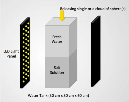
2 Experimental setup. . . 10
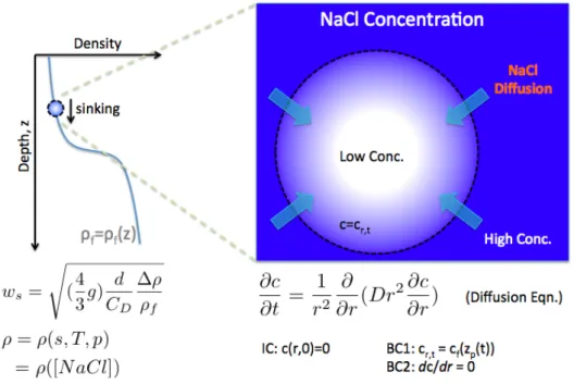
3 Schematic diagram of the numerical model. . . 12
4 Vertical trajectories of the eight agarose spheres (table 3) in a homogeneous column. . . 15
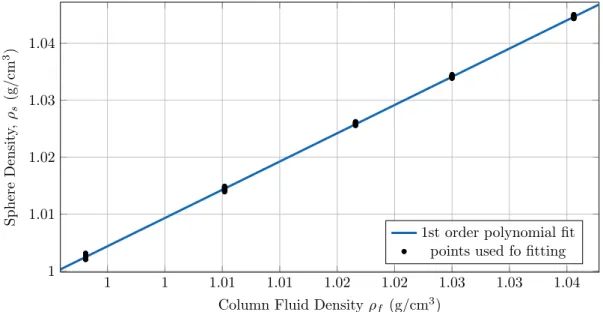
5 Linear regression between the water column density and the sphere density. . . 16
6 Density profiles of water columns used for a single sphere settling experiment. . . 17
7 Vertical trajectories of the eight agarose spheres . . . 18
8 The definition of residence time,τr. . . 20
9 τr of a settling single sphere from experiments in the stratified water columns. . . 21
10 τr of a settling single sphere from experiments in the stratified water columns. . . 21
11 Comparison of vertical trajectories of a sphere between experimental and numerical results. . . 22
12 Entrainment of fluid (adapted from Camassaet al. 2009). . . 23
13 Comparison ofτr between experimental and numerical results. . . 23
14 τr andτr/τsfrom the numerical simulation. . . 25
15 Cloud centroid vs. time. . . 27
16 τr of different clouds of spheres. . . 28
17 τr of clouds of small spheres (53–300µm in diameter). . . 28
18 Residence time of clouds of large spheres (1.00–2.80 mm in diameter). . . 29
19 Normalized residence time,τr/τs, of the clouds. . . 30
20 Power-law fitting ofτr/τs of the clouds. . . 30
21 τr of the clouds in differentN2. . . 31
22 Numerical simulation of a cloud of spheres. . . 32
24 The comparison between a large-sphere cloud and a small-sphere
cloud. . . 34 25 Centroid, standard deviation, skewness, and kurtosis of the clouds. . . 35 26 Centroid and standard deviation of a small-sphere cloud and a
large-sphere cloud. . . 37 27 The comparison of the cloud growth between the experiment and the
numerical simulation. . . 39 28 A shell of entrained fluid around a sphere. . . 40 29 Vertical trajectories of a single sphere in a 2-layered stratification from
numerical simulation with entrainment. . . 41 30 τr of a single sphere in a 2-layered stratification from numerical
simulation with entrainment. . . 41 31 Vertical trajectories of a single sphere in a linear stratification from
numerical simulation with entrainment. . . 42 32 τr of a single sphere in a linear stratification from numerical
simulation with entrainment. . . 42 33 Comparison between τr, diffusion time scale (τd), and settling time
Chapter 1
Background
Settling of marine snow, organic aggregates larger than 0.5 mm in diameter (Alldredge & Silver 1988) and a dominant form of settling particulate organic carbon (POC) (Fowler & Knauer 1986), has a central role in transporting organic carbon from the surface ocean to the interior ocean (Turner 2002). This has a direct linkage to the climate, for example, Falkowski (2000) estimated the annual export of 11–16 Gt of organic carbon from the surface to the deep ocean makes atmospheric carbon dioxide concentration 150–200 ppmv lower than the case with no primary production in the ocean. However, estimating how much organic carbon is exported is uncertain due to imperfect existing methodologies and limited sampled data (Burd et al.
2010). Studies using sediment traps, the only tool which can directly measure POC flux, gave 5.36 GtC/yr of global export production (Honjo et al. 2008). The model calculation based on the empirical relationship between sea surface temperature (SST), net primary production, and export production gave 11.1–20.9 GtC/yr depending on the model algorithms (Lawset al.2000). An alternative approach using relationship between234Th–238U and SST yielded about 5 GtC/yr (Hensonet al.2011). In contrast to many efforts to estimate the global POC flux, the physical settling process of individual POCs has been left largely unstudied. The better understanding of the physical settling processes mechanistically will contribute the better incorporation of field data and important biogeochemical processes to the model. Accordingly, it will lead to the better estimation of the global POC flux.
Gotschalk 1988). Iversen & Ploug (2010) found the excess density of marine snow to the ambient water decreases with its size, while Alldredge & Gotschalk (1988) found no correlation between them. Besides the experimental studies, models to predict settling velocity and excess density of flocculated sediment in the river and coastal environment were proposed (Kranenburg 1994; Khelifa & Hill 2006).
Table 1: Sinking rates of zooplankton fecal pellets, marine snow and phytodetritus(adapted from Turner 2002).
Regardless of whether they were experimental or in situ observational studies, the previous studies were not able to actively control the important parameters of marine snows including size, density, porosity, and shape. Considering the various origins of marine snow, ones with an identical size and shape do not necessarily have same properties. Accordingly, a systematic approach is desired to elucidate the underlying physical processes.
Deksheniekset al.2001; McManuset al. 2008; Prairieet al.2010).
Lastly, the studies based on an individual particle overlook possible interactions between particles. This issue will be especially important for the episodic settling of large numbers of particles, e.g. algal blooms.
Only a very few studies have investigated the effect of stratification on the settling of real marine particles or porous particles. MacIntyre et al. (1995) studied the vertical distribution of marine snow and its correlation with density discontinuities by analyzing observational data and using models. Kindleret al.(2010) used manufactured porous particles and they found the porous particles are trapped for some period of time at the density transition layer to exchange the interstitial and the ambient fluids by molecular diffusion. Prairie et al. (2012) conducted similar research to Kindleret al. (2010) but with natural aggregates and proposed two possible mechanisms which reduce the settling velocity of particles in the density interface: 1) by diffusion, which is also observed by Kindleret al. (2010), and 2) by entrainment of lighter fluid from the upper layer.
In this study, the settling behavior of a single and a cloud of porous spheres, which resembles the highly porous nature of marine snow, was investigated. By using manufactured porous spheres, the key factors could be studied systematically because of the exclusion of the variability and uncertainty of physical characteristics including porosity, solid matrix density, and shape.
InTheory, the governing physics will be discussed. InMethods, the experimental procedure and
the formulation of the numerical model will be introduced. InResultsandDiscussion, the results from laboratory experiment and numerical simulation will be presented and discussed. Finally,
inConclusions, the findings of this study will be summarized, and future work will be suggested.
Theory
Settling of a single porous sphere in a stratified water column
The settling of a low Reynolds number sphere is governed by the Basset-Boussinesq-Oseen (BBO) equation. When no ambient fluid motion exists, the BBO equation is expressed as
π 6ρsd
3dU dt =−
π 8ρfU
2C Dd2−
π 12ρfd
3dU dt −
3 2d
2√πρ fµ
Z t
t0 1
√
t−τ dU
dτ dτ+ π
6(ρs−ρf)d 3g (1)
whereρsis the density of the sphere,dis the diameter of the sphere,U is the settling velocity of the sphere,ρf is the density of the ambient fluid, t is time,CD is drag coefficient,µis dynamic viscosity of a fluid, and g is gravity (modified from Johnson 1998, chapter 18). The term on the left hand side is inertia, and the terms on the right hand side are drag force, added mass effect, basset force, and reduced gravity, respectively. In this study, the added mass effect and basset force are negligible (Khatri, 2012, unpublished data). Hence, equation (1) is simplified to
π 6ρsd
3dU dt =−
π 8ρfU
2C Dd2+
π
6(ρs−ρf)d
3g . (2)
As the Reynolds numbers of the spheres ranges from 0.1 to 10 in this study, a corrected Stokes drag law was used (White 1974):
CD= 24 Re+
6
1 +√Re + 0.4 (3)
(Re=ρfU d µ ).
For a stratified water column,ρf is not a constant but a function of depth,z,
ρf=ρf(z).
Accordingly, while a sphere is sinking,ρsalso changes over time since diffusive exchange occurs whenever a density difference exists between ambient fluid and the interstitial fluid of a porous sphere. The density of a porous sphere with a porosity, P, which is a volume fraction of the interstitial fluid out of the total volume of the sphere, can be defined as
ρs=P ρf0+ (1−P)ρm (4)
whereρf0 is the average density of interstitial fluid, andρmis the solid matrix density. Here,ρf0
salt concentration,C:
ρf0 =ρf0(C).
C of the interstitial fluid of a sphere can change in a stratified water column, whenever a con-centration difference exists between the ambient fluid and the interstitial fluid of the sphere. The salt concentration of the ambient fluid, Cf at the surface of a sphere, which changes over time while a sphere is settling through stratification, drives molecular diffusion of salt into the sphere. Also, the gradient of salt inside a sphere usually exists because diffusion is a slow process compared to sinking of a sphere:
C=C(r, t)
whereris the distance from the center to a point in a sphere.
The diffusive process can be described by Fick’s second law, assuming diffusion coefficient, D, is a constant.
∂C ∂t =
D r2
∂ ∂r(r
2∂C
∂r) (5)
Initial condition: C(r,0) = 0
Boundary conditions: ∂c/∂r= 0 atr= 0, and C=Cf atr=d/2
Then, the average concentration of interstitial fluid inside a sphere can be calculated.
Cavg(t) = Rd/2
0 C(r, t)πr 2dr
1 6πd
3 (6)
ρf0 =ρf0(cavg)
In this study, sodium chloride (NaCl) was used to stratify a water column. The conversion be-tweenρf0 and [NaCl] was interpolated using a density-concentration table at 20◦C(in appendix,
Mettler Toledo).
Settling of a cloud of porous spheres in a stratified water column
and the total buoyancy,Q,
Q=g0V0,
where Q is the released total buoyancy, g0 (= ρ−ρf
ρ g) is the reduced gravity, ρand V0 are the initial density and the volume of the thermal, ρf is the density of the ambient fluid, and V is the volume of the thermal. Then, dimensional study shows
b=c1z, W =c2Q1/2/z, g0=c3Q/z3,
wherebis the half horizontal length of the thermal,zis the vertical length of the front from the release point, and W is the settling speed of the thermal (Noh & Fernando 1993; Bush et al.
2003). The constants (c1,c2, andc3) can be obtained empirically.
In a homogeneous column, theoretically the thermal, which consists only of a fluid denser than the water column, can sink indefinitely satisfying the above similarity condition because it has excess negative buoyancy at any moment. However, a particle cloud, which consists of heavy particles and a fluid with density identical to that of the water column, initially forms a thermal but does not propagate indefinitely. At a certain point, the particles in the thermal will fall out, and the separated particles form a bowl-shaped cluster, which settles as a group of independent individual particle, not as a thermal (Slack 1963; Rahimipour & Wilkinson 1992; B¨uhler & Papantoniou 2001; Noh & Fernando 1993; Bushet al.2003). Accordingly, two different regimes exist: the so calledthermal regime and theparticle settling regime(Noh & Fernando 1993). Noh & Fernando’s (1993) experiment found the critical depth measured from a virtual origin,zc, where the transition between the two regimes happens, follows the relationship, zcws/ν ∼ (q/νws)α withα'0.3, wherewsis the terminal settling velocity of an individual particle,ν is kinematic viscosity, and q (= 43πa3g0N where a and ρp are the radius and the density of a particle, respectively, g0 is the reduced gravity of the particles, ρp−ρf
ρp g, and N is the number of the
released particles per unit length) is the total buoyancy of the released particles per unit length. Later, Bushet al. (2003) found another empirical relationship: zc/a= (11±2)(Q1/2/wsa)5/6.
lighter than that of the bottom layer, but it disappears soon because the particles escape while propagating and accordingly the turbidity current loses its momentum.
Bush et al. (2003) studied a cloud of particles in a linearly stratified column. They found
when the stratified cloud number,Ns=wsQ−1/4N−1/2 (Luketina & Wilkinson 1994), is bigger than unity, the cloud initially sinks as a thermal, then particles in the cloud fall out as a bowl-shaped swarm at a certain depth and the rest of fluid associated in the cloud ascends to the depth which matches its density. A vertical oscillation of the remaining fluid was observed at a frequency close to N, the buoyancy frequency of the ambient stratification. When Ns <1, the cloud initially sinks as a thermal; however, the whole cloud overshoots the neutral depth, bounces back, and intrudes at the depth of its neutral buoyancy forming a gravity current. The particles in the cloud fall out between the maximum penetration depth and the neutral depth in an irregular shape.
To the author’s knowledge, no work has been done with clouds of porous spheres, the density of which is initially lower than that of the BL fluid but higher than that of the TL fluid. If the porous sphere is large enough that the diffusive uptake of salt from the ambient fluid takes for a certain period of time until it gains an excess negative buoyancy, the porous spheres in the cloud would be temporarily trapped at their neutral depth regardless ofX orNs. On the other hand, if the porous spheres are so small that the diffusive fluid exchange occurs instantly, the settling behavior of the porous sphere cloud may be similar to the case of the solid (or non-porous) particle settling.
Methods
Experimental scheme
Porous spheres
The spheres used in this study were made of agarose. Smaller spheres (diameter: 50–300
μm) were supplied from a commercial supplier (ABT), and larger spheres were made in the
(a) (b)
Fig. 1: Manufactured agarose spheres (a) and the measurement of their sizes on a slide with 1 mm grid spacing (b).
Water column stratification
An acrylic water tank (28 cm L x 28 cm W x 60 cm H, inner dimension) was used to set up three kinds of water columns: 1) homogeneous water column, 2) sharp 2-layer stratified water column, and 3) linearly stratified water column. For a 2-layer stratification, BL fluid with a higher density was poured first, and TL fluid, which was always DI water, was introduced slowly using a diffuser, a sponge with a styrofoam rim which floats on water. For linear stratification, BL fluid was poured to a certain height, then Oster’s (1965) two vessel technique was applied to make a linearly stratified region, and finally TL fluid was introduced at the top using the diffuser. For some experiments, a same 2-layered water column sit for an extended period of time to make its stratification thicker (figure 21 (c)).
After setting up a stratified water column, temperature and conductivity were profiled every 1 cm or 0.5 cm around the density interface from the bottom to the top using a sensor (MSCTI Model 125, PME Inc.), then converted to density using Gibbs-SeaWater (GSW) Oceanographic Toolbox (McDougall & Barker 2011). However, due to the discrepancy of the composition between the real seawater and a NaCl solution, GSW Oceanographic Toolbox does not return the actual density of the NaCl solution. Accordingly, it was scaled using the actual densities of BL and TL fluids, which were measured by a density meter (DMA 35, Anton Paar).
Video imaging
taken at about 8 or 16 frames per second (figure 2). The frame size was 1,000 x 1,000 pixels at maximum with bit depth of 8 or 16 bit/pixel. The timestamp function on the software did not return the right time information due to an unknown computer error, so time information was reconstructed using an average time interval (the total number of images / [the oretime the last image was taken - the time the first image was taken]).
Experiments
Single sphere experiment. Water columns with different stratification were made, then the
Fig. 2: Experimental setup. The water tank with inner dimensions of 28 cm L x 28 cm W x 60 cm H was built of acrylic. LED lighting apparatuses were placed on each side of the tank. The water column was homogeneous or stratified according to the purpose of the experiment. A single sphere or a cloud of spheres was released from the top of the tank. For single sphere releasing experiments, an acrylic lid with a center hole sat just below the water surface in order to eliminate disturbances due to the free surface.
Cloud of spheres experiment. Experimental procedures were identical to that of the single
sphere experiment, except for the sphere preparation stage and the presence of a lid. The lid was not used, since the free surface disturbance was not as significant as in the case of the single sphere experiments. The spheres were sorted by using sieves with different mesh sizes (0.053, 0.100, 0.150, 0.180, 0.250, 0.300, 1.00, 1.40, 1.70, 2.00, 2.36, 2.80 mm, Cole-Parmer). Then, each was weighed on a balance and made into a cloud solution with a certain concentration of spheres (known weight of spheres to a total weight of the spheres and DI water). Large-sphere clouds, with the total weight of 9.2 or 10 g, were released using a stemless funnel and a plunger as decribed in Bushet al.(2003). However, clouds of small spheres, with total volume of 1 cm3, was released by a pipette slowly. The concentration of spheres in a cloud was always 25% (25% of spheres and 75% of DI water by weight).
Image processing
Preconditioning. Images were processed using MATLAB (MathWorks) and DataTank (Visual
the background image, which was usually set to be the image att= 0, was subtracted from the cropped image. Then, low-value signals under a threshold (1–2 % of the saturated value of a pixel) were removed from all pixels in each image.
Single sphere tracking. The initial location of a sphere att= 0 was picked manually, and then
the sphere was tracked automatically with the following algorithm: 1) set a small region around the sphere, 2) identify all dots in the region, 3) pick dots bigger than a certain area, which is a number of connected pixels, 4) find a dot with the largest area, which is assumed to be the sphere, and 5) if the number of dots with the largest area are more than two, find a dot which is the closest to the previous sphere position. The centroid of the connected pixels in a dot was set as a position of the sphere. Finally, the trajectory was smoothed using a Butterworth filter in order to remove fluctuations due to a fairly large pixel size that is comparable to the size of the sphere.
Cloud of spheres tracking. The centroid of the whole cloud was tracked for each image using
the following equation,
Zc(t) = Z zn
0 z
Rxn
0 i(x, z, t)dx Rxn
0 Rzn
0 i(x, z, t)dzdx !
dz (7)
whereZcis the vertical location of centroid,zn is the vertical length of the image in pixels,xn is the horizontal length of the image in pixels, andi(x, z, t) is the signal intensity at (x, z) at time t. Also, 2nd, 3rd, and 4th moments were calculated to investigate the shape of a cloud:
Standard deviation, SD(t) = v u u t
Z zn
0
(z−Zc(t))2 Rxn
0 i(x, z, t)dx Rxn
0 Rzn
0 i(x, z, t)dzdx !
dz, (8)
Skewness(t) = 1 SD(t)3
Z zn
0
(z−Zc(t))3 Rxn
0 i(x, z, t)dx Rxn
0 Rzn
0 i(x, z, t)dzdx !
dz, (9)
Kurtosis(t) = 1 SD(t)4
Z zn
0
(z−Zc(t))4 Rxn
0 i(x, z, t)dx Rxn
0 Rzn
0 i(x, z, t)dzdx !
dz. (10)
Numerical models
Sinlge sphere model
The model calculates the location of a porous sphere at each time step (schematic diagram of the model is shown in figure 3). Letting the center of ambient stratification be atz= 0 and z increases toward the direction of gravity, the settling velocity of the sphere is
wherezp is the position of the sphere. Then, it is discretized with a forward time scheme,
zpt+1=zpt+ ∆t·Ut.
dU
dt was discretized from equation (2) with forward time scheme,
Ut+1=Ut+ ∆t
−3ρfCDU
2
8ρsa
+ρs−ρf ρs
g
whereais the radius of a sphere. The initial velocity,U0, is an arbitrarily assigned small number sinceCD cannot be defined whenU = 0.
Fig. 3: Schematic diagram of the numerical model. The left shows a density profile of a stratified water column. When a porous sphere settles in a stratified water column, it experiences a change in
∆ρ, the density difference between the sphere and the ambient fluid. ∆ρis a key control factor
of settling speed. Because all experiments were performed at room temperature and the water column height was only 60 cm, density of fluid becomes a function of the concentration of salt (NaCl) in this study. As the sphere was porous, salt molecules are diffused from the ambient fluid to into the sphere since the settling sphere has lighter interstitial fluid than the ambient fluid at depth. The diffusion equation was adapted to our model with an initial condition that the salt concentration ([NaCl]) is initially zero and two boundary conditions: 1) [NaCl] of the interstitial fluid on the sphere’s surface is identical to that of the surrounding ambient fluid and 2) the gradient of [NaCl] at the center of sphere is zero.
In the presence of ambient stratification, a porous particle changes its density until equilib-rium as long as the density of interstitial fluid of a sphere (ρf0) is different than that of ambient
fluid (ρf). Diffusion equation (equation (5)) was discretized with forward time and central space schemes,
k1= D r∆r +
D
∆r2, k2=− 2D
∆r2, k3=− D r∆r+
D ∆r2,
whereCr,tis a concentration of salt at a point with a distance ofrfrom center and at time oft, ∆ris a spatial grid spacing, and ∆tis a time step spacing. The initial salt concentration of the interstitial fluid was assumed to be zero. For each time step, the boundary conditions change. To calculate theCr,t+1,C0,tandCa,twere substituted withCdr,tandCf(zp(t)), respectively.
The average concentration of salt of the interstitial fluid,Cavg, was calculated using equation (6),
Cavg(t) = nr−2
X
i=0 4
3π[(dr·(i+ 1))
3−(dr·i)3]Cdr·(i+1),t−Cdr·i,t 2
where nr is the number of spatial grid points along the radial axis, and dr is the spatial grid spacing. Then,Cavg was converted toρf0. Then,ρswas calculated using equation (4).
White’s (1974) empirical drag law (equation (3)) was used for CD. The ambient density profileρf was approximated to a fitted curve from each experiment. An error function fit was used for 2-layered stratification,
ρf(z/
√
4Dt∗) =ρf+∆ρf
2 erf(z/
√
4Dt∗)
wheret∗is the characteristic time which best fits the measured density profile. Also, a piecewise
cubic Hermite interpolating polynomial function fit was used for linear stratification.
Cloud model
Results
Three main sets of laboratory experiment were conducted to investigate the settling behavior of porous spheres in the present of stratification: 1) settling of single spheres in homogeneous water columns, 2) settling of single spheres in stratified water columns, and 3) settling of sphere clouds in stratified water column. Porous spheres made of agarose were used as a proxy for marine snow, and sodium chloride was used as a stratifying agent. By using these laboratory-manufactured spheres, the potential uncertainties caused by the irregular shape, porosity, and solid matrix density of real marine snow could be excluded while maintaining key parameters (e.g. porosity and stratification type). The parameters utilized in the experiments were sphere size, type of density stratification, and porosity (table 2). In addition, numerical simulation was conducted to demonstrate both settling of a single sphere and of a cloud of spheres. Then, results from the lab experiments were compared with that from the numerical simulation.
ID Radius (mm) ρT L(g/cm3) ρBL(g/cm3) Homogeneous Column
1†
table 3
0.9982 —
2† 1.0108 —
3† 1.0216 —
4† 1.0300 —
5† 1.0407 —
2-Layer Column 6
table 3 0.9987 1.0214
7 0.9982 1.0413
Linear Column 8
table 3 0.9982 1.0216
9 0.9986 1.0407
(a)Single sphere experiment list. (†: the experiment were repeated three times.)
ID Diameter (mm) Releasing Amount Sphere
Concentration (%) ρT L (g/cm3)
ρBL (g/cm3) 2-Layer Column
10 1.00–1.40, 1.40–1.70, 1.70–2.00 2.00–2.36, 2.36–2.80
10 g
25% spheres + 75% TL fluid
0.9979 1.0225
11 10 g 0.998 1.02
12‡ 0.150–0.106, 1.40–1.70 1ml, 9.2g 0.9983 1.0220
13
0.053–0.106, 0.106–0.150 0.180–0.250, 0.250–0.300
1ml 0.9980 1.040
14 1ml 0.9980 1.0201
15 1ml 0.9980 1.0101
(b)Cloud experiment list. (‡: the experiment was conducted with five different density interface
thick-nesses.)
Table 2: List of experiments.
Homogeneous column experiment
repetitive experiments were done.
Sphere ID 1 2 3 4 5 6 7 8
Radius (mm) 0.4266 0.4451 0.5380 0.6260 0.6576 0.7826 0.8512 0.9413 Rein Fresh Water 1.3246 1.5287 2.3631 3.4739 3.8325 5.6344 6.9021 8.5932
Table 3: Agarose spheres used for a single sphere experiment. The ID, radius, and Reynolds number of each sphere are shown in the first, second, and third rows, respectively.
The vertical position of a sphere was plotted for the entire time domain. However, in some cases, fluctuation existed near the bottom. Accordingly, the top 50 pixels and the bottom 300 pixels were cropped (figure 4). The trajectories in the cropped region were each fit with a line by the least squares method, and the slope of each curve was the terminal settling velocity,ws. As each experiment was repeated three times, the mean value of the three became the final settling velocity used for further analysis.
0 50 100 150 200 250 300 350 400
0
200
400
600
800
1,000
Time,t (s)
V
ertical
P
osition,
z
(p
x)
1 2 3 4 5 6 7 8
Fig. 4: Vertical trajectories of the eight agarose spheres (table 3) in a homogeneous column with 1.0406
g/cm3. Each different color marks a different sphere whose ID number is shown in the box at
the top right corner. Only the middle section between the two dashed lines was used to calculate the settling velocity of each sphere.
Equation (2) withdU/dt= 0 andU =ws is rearranged to
ρs= (3CDws 2
4dg + 1)ρf.
The total density of each sphere was calculated with the above equation usingwsfrom experi-ment.
between ρ0f and ρs using equation (4). As the spheres were hydrated in the same fluid of the water column before experiment,ρ0
fwas identical toρf. The porosity was 0.9916 and the matrix density was 1.5215 g/cm3(figure 4). These values were used for the numerical model simulation.
1 1 1.01 1.01 1.02 1.02 1.03 1.03 1.04
1 1.01 1.02 1.03 1.04
Column Fluid Densityρf (g/cm3)
Sphere
Densit
y
,
ρs
(g/cm
3)
1st order polynomial fit points used fo fitting
Fig. 5: Linear regression between the water column density and the sphere density.
Ac-cording to equation (4), the slope of the linear regression line is the porosity (P)
of agarose spheres, and the y-intersect is the product of (1 − P) and the
den-sity of matrix, ρm. P = 0.9916 with 95% confidence interval [0.9886,0.9947], ρm =
1.5215 with 95% confidence interval [0.8624,2.1806], R2= 0.9997.
2-Layer stratification experiment
1 1.01 1.02
−10
0
10
Density (g/cc)
Depth
(cm)
Fit Raw
(a)2 Layer (BL 1.0216 g/cc)
1 1.02 1.04
−10
−5
0
5
10
Density (g/cc)
Depth
(cm)
Fit Raw
(b)2 Layer (BL 1.0406 g/cc)
1 1.01 1.02
−10
0
10
20
Density (g/cc)
Depth
(cm)
Fit Raw
(c)Linear (BL 1.0216 g/cc)
1 1.02 1.04
−20
−10
0
10
20
Density (g/cc)
Depth
(cm)
Fit Raw
(d)Linear (BL 1.0406 g/cc)
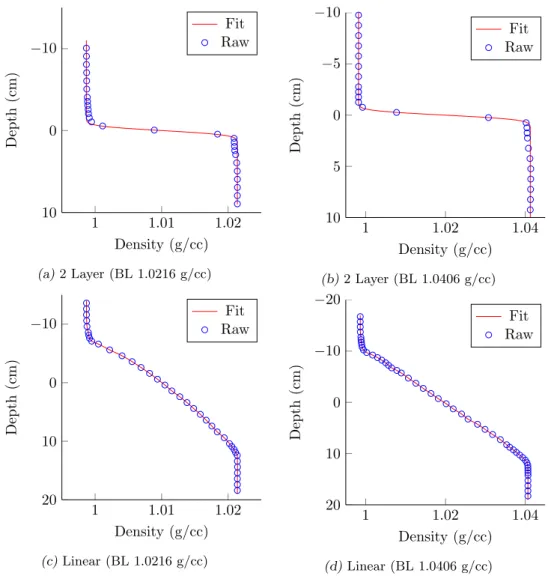
Fig. 6: Density profiles of water columns used for a single sphere settling experiment. The blue circles are the measured densities using a CT probe, and the red lines are the fitted curves—an error function was used for a and b, and a piecewise cubic Hermite interpolating polynomial function
was used for c and d. ρtopwas always fresh water, whileρbottomwas 1.0216 g/cm3 (a and c) and
1.0406 g/cm3 (b and d). Experiments were done in both sharp 2-layered stratification (a and b)
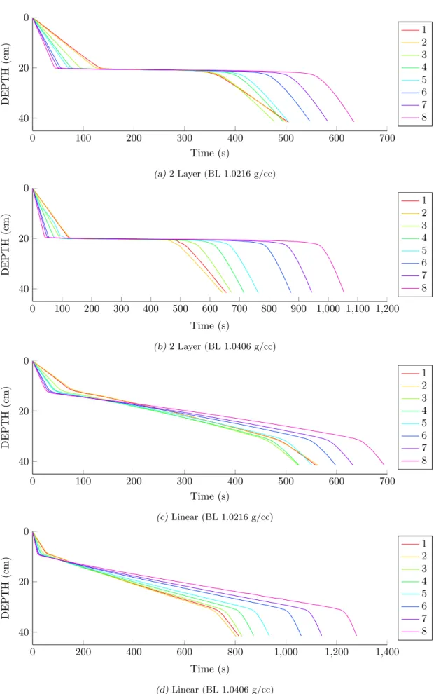
0 100 200 300 400 500 600 700 0 20 40 Time (s) DEPTH (cm) 1 2 3 4 5 6 7 8
(a)2 Layer (BL 1.0216 g/cc)
0 100 200 300 400 500 600 700 800 900 1,000 1,100 1,200 0 20 40 Time (s) DEPTH (cm) 1 2 3 4 5 6 7 8
(b)2 Layer (BL 1.0406 g/cc)
0 100 200 300 400 500 600 700
0 20 40 Time (s) DEPTH (cm) 1 2 3 4 5 6 7 8
(c)Linear (BL 1.0216 g/cc)
0 200 400 600 800 1,000 1,200 1,400
0 20 40 Time (s) DEPTH (cm) 1 2 3 4 5 6 7 8
(d)Linear (BL 1.0406 g/cc)
The single most important parameter is a time scale of delayed settling due to stratification, because it has important ecological implications—e.g. the amount of POC remineralized or consumed by microbes and zooplankton is related to the time that POC spends in the water column. To measure the time scale, residence time,τr, was introduced (figure 8). τrwas defined as the time taken to settle through a stratified region. The stratified region was defined as the region where the local density gradient is equal to or greater than one thousandth the maximum local density gradient (z where dρf
dz ≥0.001max( dρf
dz ), figure 8 (c)). In addition, residence time normalized by settling time scale, τr/τs, was used when necessary. The settling time scale, τs was defined as
τs=1 2(
lbox wT L +
lbox
wBL) (11)
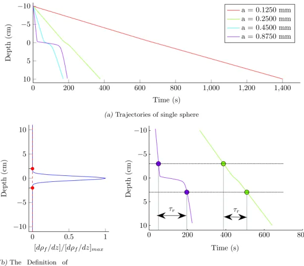
0 200 400 600 800 1,000 1,200 1,400
−10
−5
0 5 10
Time (s)
Depth
(cm)
a = 0.1250 mm a = 0.2500 mm a = 0.4500 mm a = 0.8750 mm
(a)Trajectories of single sphere
0 0.5 1
−10
−5
0 5 10
[dρf/dz]/[dρf/dz]max
Depth
(cm)
(b)The Definition of
Stratified Region
0 200 400 600 800
−10
−5
0
5
10
Time (s)
Depth
(cm)
τr τr
(c)Residence Time
Fig. 8: The definition of residence time, τr. The vertical position of a sphere over time (from the
numerical simulation using profile of figure 6 (a), where the center of stratification is located at the zero depth) is shown in (a). The vertical length of the density region is defined as the
region wheredρf/dzis equal to or higher than 0.1% of the maximumdρf/dz(b). The residence
time is the difference in two time points when a sphere passes the upper boundary and the lower boundary of the density interface (c).
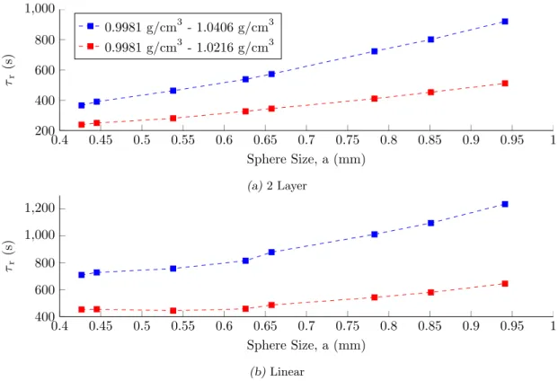
0.4 0.45 0.5 0.55 0.6 0.65 0.7 0.75 0.8 0.85 0.9 0.95 1 200
400 600 800 1,000
Sphere Size, a (mm) τr
(s)
0.9981 g/cm3 - 1.0406 g/cm3 0.9981 g/cm3 - 1.0216 g/cm3
(a)2 Layer
0.4 0.45 0.5 0.55 0.6 0.65 0.7 0.75 0.8 0.85 0.9 0.95 1
400 600 800 1,000 1,200
Sphere Size, a (mm) τr
(s)
(b)Linear
Fig. 9: τrof a settling single sphere from experiments in 2-layer stratification (a) and in linear
stratifica-tion (b). The density difference between top and bottom layers (∆ρf) was∼0.04 g/cm3 (blue)
and∼0.02 g/cm3 (red). The spheres in table 3 were used.
0.4 0.45 0.5 0.55 0.6 0.65 0.7 0.75 0.8 0.85 0.9 0.95 1
200 400 600
Sphere Size, a (mm) τr
(s)
Linear stratification 2-layered stratification
(a)(BL 1.0216 g/cc)
0.4 0.45 0.5 0.55 0.6 0.65 0.7 0.75 0.8 0.85 0.9 0.95 1
400 600 800 1,000 1,200
Sphere Size, a (mm) τr
(s)
(b)(BL 1.0406 g/cc)
Fig. 10: τr of a settling single sphere from experiments in ∆ρf ∼= 0.02 (a), ∆ρf ∼= 0.04 (b). Water
column stratification was linear (blue) and 2-layered (red). This figure and figure 9 share same data, but organized differently. The spheres in table 3 were used.
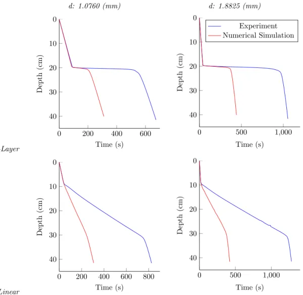
per-fectly. However, it seems to predict the tendency well, although the τr was significantly lower in the numerical simulation result than the experimental result (figure 13). The main reason is likely to be the entrainment of the buoyant TL fluid (Srdic-Mitrovic et al. 1999; Abaid et al.
2004; Camassaet al.2009, 2010). The entrained fluid from the TL forms a shell of lighter fluid (figure 12) around a sphere, which acts as a barrier to molecular diffusion. Because the [NaCl] of the entrained fluid is lower than that of the ambient fluid, it slows down the diffusive exchange process.
d: 1.0760 (mm) d: 1.8825 (mm)
2-Layer
0 200 400 600
0
10
20
30
40
Time (s)
Depth
(cm)
0 500 1,000
0
10
20
30
40
Time (s)
Depth
(cm)
Experiment Numerical Simulation
Linear
0 200 400 600 800
0
10
20
30
40
Time (s)
Depth
(cm)
0 500 1,000
0
10
20
30
40
Time (s)
Depth
(cm)
Fig. 11: Comparison of vertical trajectories between experimental (blue) and numerical (red) results
in 2-layer stratification (top) and linear stratification (bottom) with ∆ρf ∼= 0.04g/cm3. Left
Fig. 12: Entrainment of fluid (adapted from Camassaet al.2009). A sphere with 0.635 cm radius and a density heavier than BL fluid was released from the top in a stratified fluid column in a acrylic cylinder with 9.45 cm radius. The pictures were taken every 10 seconds. The TL fluid was the
mixture of pure corn syrup and dye with the density of 1.37661 g/cm3, while the BL fluid was
the mixture of pure corn syrup and salt with the density of 1.38384 g/cm3.
BL: ∼=1.02 g/cm3 BL: ∼=1.04 g/cm3
2-Layer
0.4 0.6 0.8 1
0 200 400 600
Sphere Size, a (mm)
Residence
T
im
e
(s)
Experiment Numerical Simulation
0.4 0.6 0.8 1
0 500 1,000
Sphere Size, a (mm)
Residence
T
im
e
(s)
Linear
0.4 0.6 0.8 1
0 200 400 600
Sphere Size, a (mm)
Residence
T
im
e
(s)
0.4 0.6 0.8 1
0 500 1,000
Sphere Size, a (mm)
Residence
T
im
e
(s)
Fig. 13: Comparison ofτr between experimental (blue) and numerical (red) results in 2-layer
stratifica-tion (top) and linear stratificastratifica-tion (bottom). The density difference between top and bottom
layers (∆ρf) is∼0.02 g/cm3 (left) and∼0.04 g/cm3 (right). The spheres in table 3 were used.
small particle was not implementable with the current experimental setup. In addition, porous spheres in this size range could not be manufactured with the same method in the laboratory. When a sphere is smaller than a certain size,τrdecreases with the size of the sphere (figure 14 (a) and (c)). On the other hand, the opposite is true for a sphere that is larger than a certain size. When a porous sphere is smaller than a certain size, it seems that a diffusive process is less important for a smaller sphere than a larger sphere that because equilibration occurs relatively faster due to a lesser volume of interstitial fluid. In such a case, physical settling rates would be more important. A smaller sphere has a smaller settling velocity, and accorindingly, it has a longer time to settle through the stratified region. This can be also seen usingτr/τs (figure 14 (b) and (d))—for smaller spheres,τr/τsis∼1.
τr τr/τs
2-Layer
0 0.5 1 1.5
0 200 400 600 800
Sphere size, a (mm)
Residence
Time
(s)
∆ρf ∼= 0.04 g/cm 3
∆ρf ∼= 0.02 g/cm3
0 0.5 1 1.5
0 50 100 150 200 250
Sphere size, a (mm)
Normalized
Residence
Time
(a) (b)
Linear
0 0.5 1 1.5
0 500 1,000 1,500 2,000 2,500
Sphere size, a (mm)
Residence
T
im
e(s)
0 0.5 1 1.5
0 5 10 15 20 25
Sphere size, a (mm)
Normalized
Residence
Time
(c) (d)
Fig. 14: τr andτr/τs from the numerical simulation. The water column density profile of experiment
#6–9 in table 2 was used (figure 6). The vertical lengths of density interface region was 3.09 (blue) and 3.97 (red) cm for 2-layer stratifications (top) and 26.00 (blue) and 29.00 (red) cm for linear stratifications (bottom).
Settling of a cloud of porous spheres
0 100 200 300 400 500 600 700 800 900 1,000 1,100 1,200 0 10 20 30 Time (s) Depth (cm) 0.250-0.300 mm 0.180-0.250 mm 0.106-0.150 mm 0.053-0.106 mm
(a)Small-sphere cloud in 2-layer stratification (∆ρ∼= 0.01g/cm3).
0 200 400 600 800 1,000 1,200 1,400 1,600 1,800 2,000 2,200 2,400 0 10 20 30 Time (s) Depth (cm) 0.250-0.300 mm 0.180-0.250 mm 0.106-0.150 mm 0.053-0.106 mm
(b)Small-sphere cloud in 2-layer stratification (∆ρ∼= 0.02g/cm3).
0 100 200 300 400 500 600 700 800 900 1,000 1,100 1,200 1,300 1,400 0 10 20 30 Time (s) Depth (cm) 0.250-0.300 mm 0.180-0.250 mm 0.106-0.150 mm 0.053-0.106 mm
(c)Small-sphere cloud in 2-layer stratification (∆ρ∼= 0.04g/cm3).
0 100 200 300 400 500 600 700 800 900 1,000 1,100 1,200 1,300 1,400 0 20 40 Time (s) Depth (cm) 2.36-2.80 mm 2.36-2.00 mm 1.70-2.00 mm 1.40-1.70 mm 1.00-1.40 mm
(d)Largel-sphere cloud in 2-layer stratification (∆ρ∼= 0.02g/cm3).
0 50 100 150 200 250 300 350 400 450 500 550 600
0 20 40 Time (s) Depth (cm) 2.36-2.80 mm 2.36-2.00 mm 1.70-2.00 mm 1.40-1.70 mm 1.00-1.40 mm
(e)Largel-sphere cloud in 2-layer stratification (∆ρ∼= 0.02g/cm3).
Fig. 15: Cloud centroid vs. time. ∆ρf was ∼ 0.02g/cm3 in both experiments. The total releasing
amount was 1 cm3 (a, b, and c) and 8–10 g (d and e), while the sphere concentration was same
10−1 100 0
200 400 600 800 1,000 1,200
Median Diameter of Sphere (mm) τr
(s)
4% Agarose,∆ρf=0.01g/cm 3
4% Agarose,∆ρf=0.02g/cm3 4% Agarose,∆ρf=0.04g/cm
3
1% Agarose,∆ρf=0.02g/cm3 2% Agarose,∆ρf=0.02g/cm
3
1% Agarose,∆ρf=0.02g/cm3 (s.) 1% Agarose,∆ρf=0.04g/cm
3 (s.)
Fig. 16: τr of different clouds of spheres. τr of single sphere experiment are also plotted for comparison
(yellow and dark grey). More details are in figure 17 and figure 18.
7.95·10−2 0.13 0.22 0.28
0 200 400 600 800
Median Diameter of Sphere (mm) τr
(s)
∆ρf=0.01g/cm 3
∆ρf=0.02g/cm3 ∆ρf=0.04g/cm
3
Fig. 17: τr of clouds of small spheres (53–300 µm) in different ∆ρf. The total volume of each cloud
was 1 cm3 (25% of spheres and 75% of TL fluid (w/w)). The size range of each cloud was
53–106, 106–150, 180–250, 250–300µm in diameter. Different colors show different ∆ρf. The
1.2 1.55 1.85 2.18 2.58 200
400 600 800 1,000
Median Diameter of Sphere (mm) τr
(s)
1% Agarose, ∆ρf=0.02g/cm 3
2% Agarose, ∆ρf=0.02g/cm3 1% Agarose (s.), ∆ρf=0.02g/cm
3
1% Agarose (s.), ∆ρf=0.04g/cm3
Fig. 18: Residence time of clouds of large spheres (1.00–2.80 mm in diameter) with different porosity. Porosity of spheres was higher for 1% agarose spheres (blue) than 2% agarose spheres (red). The total weight of each cloud was 8–10 g (25% of spheres and 75% of TL water (w/w)). The size range of each cloud was 1.00–1.40, 1.40–1.70, 1.70–2.00, 2.00–2.36, 2.36–2.80 mm in diameter.
τr of single sphere experiment are also plotted for comparison (yellow and dark grey).
10−1 100 100
101 102
Median Diameter of Sphere (mm) τr
/
τs
4% Agarose,∆ρf=0.01g/cm3 4% Agarose,∆ρf=0.02g/cm
3
4% Agarose,∆ρf=0.04g/cm3 1% Agarose,∆ρf=0.02g/cm
3
2% Agarose,∆ρf=0.02g/cm3
Fig. 19: Normalized residence time,τr/τs, of the clouds of spheres.
100 100.1 100.2 100.3 100.4 101
102
Median Diameter of Sphere (mm) τr
/
τs
1% Agarose, ∆ρf=0.02g/cm3 2% Agarose, ∆ρf=0.02g/cm3 1% Agarose (s.), ∆ρf=0.02g/cm3 1% Agarose (s.), ∆ρf=0.04g/cm3
τr/τs ∼ d2.487 τr/τs ∼ d2.427 τr/τs ∼ d2.504 τr/τs ∼ d2.699
Fig. 20: Power-law fitting ofτr/τs of the clouds of spheres. τr of the clouds of spheres (blue and red)
and the single spheres (yellow and dark grey).
4.21 5.37 6.14 8.62 15.2 500
1,000 1,500
N2 (1/s2) τr
(s)
Dia.: 1.40-1.70(mm) Dia.: 0.106-0.150(mm)
4.21 5.37 6.14 8.62 15.2 0
10 20 30
N2 (1/s2) τr
/
τs
(a) (b)
1 1 1.01 1.01 1.02 1.02 1.03
−10
−5
0 5 10
Density (g/cm3)
Depth
(cm)
N2=15.2(s-2) N2=8.62(s-2) N2=6.14(s-2) N2=5.37(s-2) N2=4.21(s-2)
(c)
Fig. 21: τr of the clouds in differentN2. The dotted line in red showsτr (a) andτr/τs(b) from clouds
of large spheres of 1% agarose, and the dotted line in blue shows a result from clouds of small spheres of 4% agarose in the five different stratifications (c). Releasing amount was 9.2g for a
large sphere cloud and 1 cm3 for a small sphere cloud, while the concentration of spheres in
both clouds was identical (25% of spheres + 75% of TL water (w/w)). ∆ρf was∼0.02 g/cm3.
The numerical model of a porous sphere cloud was an ensemble of numerical simulation results of individual spheres (figure 22). The settling of individual spheres of various sizes with a uniform increment was simulated, and a sphere of each different size was weighted using a hypothetical size distribution. Then, the distribution of all spheres were recorded at every time step.
decreases since the initial momentum is diluted with entrained ambient fluid over time. However, the numerical model assumes every sphere in a cloud was initially at rest and accordingly had zero momentum. Hence, the numerical model result did not reproduce the same evolution of the sinking process.
Second,τris significantly shorter in the numerical simulation result than in the experimental result (figure 23). The numerical model is an ensemble of results from single sphere settling model simulations, so it inherently has the same problem as the single sphere model—the absence of entrainment of lighter fluid from the top layer. However, it predicted the overall tendency ofτr over the sphere size in clouds (figure 23).
0 50 100 150 200 250 300
0
20
40
Time (s)
Depth
(cm)
(a)
1.7 1.8 1.9 2
2 4
·10−2
Radius (mm)
Probabilit
y
Densit
y
(b)
0 100 200 300 400 500 600 700 800 900 1,000
0
20
40
Time (s)
Depth
(cm)
Experiment Numerical Simulation
(c)
Fig. 22: Numerical simulation of a cloud of spheres. (a) Trajectories of individual spheres (d: 1.71– 2.00 mm with 0.01 mm increment) from numerical simulation. The size distribution is shown on the right graph. Color scheme corresponds. (b) Size distribution (pdf) of spheres in a
cloud. Normal distribution was assumed with dmean = dmedian and 2σ = dmedian−dmin.
(c) Comparison between experiment and numerical simulation. Experiment conditions were
∆ρf ∼= 0.02g/cm3, sphere size range: 1.70–1.20 mm, and releasing amount 10g (2.5g sphere +
1.00–1.400 1.40–1.70 1.70–2.00 2.00–2.36 2.36–2.80 200
400 600 800 1,000 1,200
Sphere diamter range in a cloud (mm) τr
(s)
Experiment Numerical Model
Fig. 23: Comparison between the experiment and numerical results of the clouds. Experimental
condi-tions were ∆ρf ∼= 0.02g/cm3, sphere size range 1.70–2.00 mm, and releasing amount 10g (2.5g
sphere + 7.5g TL water) as found in #10 in table 2.
0 16.5 33 49.5 0 16.5 33 49.5 0 0.1 0.2 0.3 0.4 0.5 0.6 0.7 0.8 0.9 1 0 16.5 33 49.5 0 16.5 33 49.5 0 0.1 0.2 0.3 0.4 0.5 0.6 0.7 0.8 0.9 1
(a)Zc= 8(cm),tL= 2.15(s),tR= 23.5(s) (d)Zc= 26(cm),tL= 140(s),tR= 617(s)
0 16.5 33 49.5 0 16.5 33 49.5 0 0.1 0.2 0.3 0.4 0.5 0.6 0.7 0.8 0.9 1 0 16.5 33 49.5 0 16.5 33 49.5 0 0.1 0.2 0.3 0.4 0.5 0.6 0.7 0.8 0.9 1
(b)Zc= 13(cm),tL= 5.57(s),tR= 51.5(s) (e)Zc= 26(cm),tL = 712(s),tR= 808(s)
0 16.5 33 49.5 0 16.5 33 49.5 0 0.1 0.2 0.3 0.4 0.5 0.6 0.7 0.8 0.9 1 0 16.5 33 49.5 0 16.5 33 49.5 0 0.1 0.2 0.3 0.4 0.5 0.6 0.7 0.8 0.9 1
(c)Zc= 24(cm),tL= 27.2(s),tR= 436(s) (f)Zc= 31(cm),tL= 838(s),tR= 1210(s)
Fig. 24: The comparison between a large-sphere cloud and a small-sphere cloud. Zc: position of centroid,
tL: the record time for left pictures, andtR: the record time for right pictures. In each pair of
pictures, the left one is a cloud with 1.70–2.00 mm spheres, and the right one is a cloud with 0.106–0.150 mm spheres (more details are in table 2 #10 and #15). For better visualization,
the intensity was amplified 1.5×and 3×respectively for large-sphere cloud and small-sphere
cloud pictures.
interface, but not to zero. This is because the spheres in small- and large- sphere clouds are in different regimes—settling regime and diffusion regime, respectively.
0 20 40 60 80 0 10 20 30 σ(cm) Cen troid (cm)
0 5001,0001,5002,000 0 10 20 30 Time (s) Cen troid (cm) 0.250-0.300 mm 0.180-0.250 mm 0.106-0.150 mm 0.053-0.106 mm
0 10 20
0 10 20 30 γ Cen troid (c m)
0 200 400 0 10 20 30 κ Cen troid (cm) (a)
0 50 100 150 200 0 20 40 σ (cm) Cen troid (c m)
0 5001,0001,5002,000 0 20 40 Time (s) Cen troid (cm ) 2.36-2.80 mm 2.36-2.00 mm 1.70-2.00 mm 1.40-1.70 mm 1.00-1.40 mm
−20 0 20 40 0 20 40 γ Cen troid (cm) 0 1,0002,000 0 20 40 κ Cen troid (cm) (b)
0 2 4 6 8 10 0 20 40 σ(cm) Cen troid (cm )
0 100 200 300 400 0 20 40 Time (s) Cen troid (c m)
−6−4−2 0 2 0 20 40 γ Cen troid (c m)
0 20 40
0 20 40 κ Cen troid (cm) (c)
Fig. 25: Centroid (in the first column), standard deviation (in the second column), skewness (in the
third column), and kurtosis (in the fourth column) of the clouds of spheres. (a) Small-sphere
clouds (#14 in table 2). (b) Large-sphere clouds (#10 in table 2). (c) Large-sphere clouds
0 500 1000 1500 0
10
20
30
40
Time (s)
Depth
(cm)
centroid +−σ stratification
(a)
0 200 400 600 800
0 10 20 30 40 50
Time (s)
Depth
(cm)
(b)
Fig. 26: Centroid and standard deviation of a cloud with 0.106–0.150 mm spheres (a) and 1.70–2.00 mm
spheres (b) in 2-layer stratification (∆ρf = 0.02 g/cm3). The stratified regions are within the
two dotted lines. The red line is the centroid, and the green region shows the±one standard
deviation of the cloud.
On the other hand, the same pattern of the different moments was not observed in the small-sphere clouds, although their standard deviation was minimum around the density interface (figure 25 (a)). This is likely to be due to the absence of pancaking at the density interface. However, the slight decrease of standard deviation and the small increase of kurtosis around the density interface would indicate that the diffusive exchange of lighter interstitial fluid and denser ambient fluid still happens, although it is in a settling regime. The skewness of the small-sphere clouds generally decreases over depth.
d= 1.70−2.00(mm) d= 2.36−2.80(mm)
0 0.02 0.04 0.06
0 5 10 15 20 25 30 35 40 45 50
N o r m a l i z e d I n t e n s i ty
D e p t h ( c m ) Model Experiment Centroid 0 0.1 0.2 0.3 0.4 0.5 0.6 0.7 0.8 0.9 1
0 0.01 0.02 0.03 0.04 0 5 10 15 20 25 30 35 40 45 50
N or m al i z e d I n t e n s i ty
D e p t h ( c m ) Model Experiment Centroid 0 0.1 0.2 0.3 0.4 0.5 0.6 0.7 0.8 0.9 1
(a)Zc = 13(cm),tm= 26.9(s),texp= 5.6(s) (b)Zc = 13(cm),tm= 41.8(s),texp= 7.97(s)
0 0.1 0.2 0.3 0.4 0 5 10 15 20 25 30 35 40 45 50
N or m al i z e d I n t e n s i ty
D e p t h ( c m ) Model Experiment Centroid 0 0.1 0.2 0.3 0.4 0.5 0.6 0.7 0.8 0.9 1
0 0.05 0.1 0.15 0.2 0 5 10 15 20 25 30 35 40 45 50
N o r m a l i z e d I n t e n s i ty
D e p t h ( c m ) Model Experiment Centroid 0 0.1 0.2 0.3 0.4 0.5 0.6 0.7 0.8 0.9 1
(c)Zc= 26(cm),tm= 105.3(s),texp= 140.1(s) (d)Zc= 26(cm),tm= 91.0(s),texp= 139.2(s)
0 0.02 0.04 0.06
0 5 10 15 20 25 30 35 40 45 50
N o r m a l i z e d I n t e n s i ty
D e p th ( c m ) Model Experiment Centroid 0 0.1 0.2 0.3 0.4 0.5 0.6 0.7 0.8 0.9 1
0 0.01 0.02 0.03 0.04 0 5 10 15 20 25 30 35 40 45 50
N or m al i z e d I n t e n s i ty
D e p th ( c m ) Model Experiment Centroid 0 0.1 0.2 0.3 0.4 0.5 0.6 0.7 0.8 0.9 1
(e)Zc= 31(cm),tm= 218.6(s),texp= 808.1(s) (f)Zc= 31(cm),tm= 109.8(s),texp= 1147(s)
Discussion
Entrainment of fluid around a sphere
To test if entrainment can prolong the residence time of a settling sphere in stratified envi-ronment, numerical simulation was performed with a modified momentum equation. Assuming the thickness of entrained fluid shell is fixed during the settling of a sphere, the entrained fluid shell was added in inertia and reduced gravity terms in equation (2):
M∗dU dt =−
π 8ρfU
2CDd2+M∗g−ρfV∗g (12)
whereM∗is the total mass of sphere and entrained fluid, π6ρsd3+π6ρf(d∗3−d3),V∗is the total volume of sphere and entrained fluid, π
6ρfd
∗3, and d∗ is the outer diameter of entrained fluid
shell (figure 28).
d∗ d
Fig. 28: A shell of entrained fluid around a sphere. A shell of entrained fluid (blue) wraps up a porous
sphere (gray). d∗is an effective diameter of the settling sphere with a diameter ofd.
In the modified numerical simulation, a porous sphere with an entrained fluid shell stayed longer within a stratified zone (figure 29 and figure 31). A larger entrained shell made τr larger for all spheres; however, the normalized thickness of an entrained fluid shell ((d∗−d)/d), which matches τr from laboratory experiment, decreases with the size of a sphere in the 2-layered stratification (e.g. τr of the smallest sphere from laboratory experiment lies between that from numerical simulation with d∗ = 1.4d and d∗ = 1.5d, while τr of the largest sphere from laboratory experiment lies between that from numerical simulation with d∗ = 1.2d and d∗= 1.3din figure 30). However, in the linear stratification, it does not decrease monotonically
with a sphere size, but increase with a sphere size and then decrease beyond a certain sphere size (figure 32).
size of sphere which is one of important variables determining settling velocity, can be directly related to the thickness of the entrained fluid shell. In such a case, the thickness of an entrained fluid shell will be adjusted according to the settling velocity of the sphere. This needs further investigation since it contradicts the assumption of the fixed thickness of the entrained fluid shell.
0 100 200 300 400 500 600 700
−20
−10
0
10
20
Time (s)
Depth
(cm)
experiment d*=1.1d d*=1.2d d*=1.3d d*=1.4d d*=1.5d d*=1.6d
Fig. 29: Vertical trajectories of a agarose sphere with diameter, 0.1076 cm, from laboratory experiment (black) and numerical simulation with different entrained fluid shell thicknesses (colored). The
experiment was performed in the 2-layered water column (∆ρf = 0.02 g/cm3, #6 in table 2).
The numerical simulation was performed with a stratification and a sphere size identical to the experiment condition.
8·010−2 0.1 0.12 0.14 0.16 0.18 0.2
500 1,000 1,500
Sphere Diameter (cm) τr
(s)
experiment d*=1.1d d*=1.2d d*=1.3d d*=1.4d d*=1.5d d*=1.6d
Fig. 30: τr of a agarose sphere from laboratory experiment (black) and numerical simulation with
dif-ferent entrained fluid shell thicknesses (colored). The experiment was performed with eight
agarose spheres (table 3) in the 2-layered water column (∆ρf = 0.02 g/cm3, #6 in table 2).
0 100 200 300 400 500 600 700
−20
−10
0
10
20
Time (s)
Depth
(cm)
experiment d*=1.1d d*=1.2d d*=1.3d d*=1.4d d*=1.5d d*=1.6d
Fig. 31: Vertical trajectories of a agarose sphere with diameter, 0.1076 cm, from laboratory experiment (black) and numerical simulation with different entrained fluid shell thicknesses (colored). The
experiment was performed in the linear water column (∆ρf = 0.02 g/cm3, #8 in table 2).
The numerical simulation was performed with a stratification and a sphere size identical to the experiment condition.
8·10−2 0.1 0.12 0.14 0.16 0.18 0.2
500 1,000 1,500
Sphere Diameter (cm) τr
(s)
experiment d*=1.1d d*=1.2d d*=1.3d d*=1.4d d*=1.5d d*=1.6d
Fig. 32: τr of a agarose sphere from laboratory experiment (black) and numerical simulation (colored).
The experiment was performed with eight agarose spheres (table 3) in the linear water
col-umn (∆ρf = 0.02 g/cm3, #8 in table 2). The numerical simulation was performed with a
stratification and a sphere size identical to the experiment condition.
The settling velocity in both the top and bottom layers increases when the entrainment of a fluid shell is included (e.g. compare the black and blue lines in figure 29). This would be resulted from our rough assumption about entrainment, but it might be attributed to the way that the entrainment was incorporated in the momentum equation. In equation (12), the entrainment was introduced to the inertia and buoyancy terms, but not to the drag term.
V-shaped trend of τr
can be roughly interpreted as the sum of the settling time scale,τsand the diffusion time scale, τd (defined as a2/2D) (figure 33). In the numerical simulation with zero entrainment, when the spheres were very small, the τr was exactly identical to τs because τd was comparatively negligible. However, when the spheres were large, the trend ofτrwas dictated by that ofτd, but the values ofτrand (τd+τs) did not match. This would be due to the simple representation of τdand the exclusion of the entrainment of lighter fluid in the vicinity of a sphere (Srdic-Mitrovic
et al. 1999; Abaid et al. 2004; Camassa et al. 2009; Yick et al. 2009; Camassa et al. 2010).
Nonetheless, the shift in dominant physical phenomena controllingτrover the sphere size range can be observed. The transition point between the settling regime (τr ∼τs) and the diffusion regime (τr∼τd) lies somewhere around the sizes whereτs=τd. It seems that, in a given water column depth and a given stratification, neither a very small nor very large particle stays the shortest time in the ocean, but some particle size in the middle does.
BL: ∼=1.02 g/cm3 BL: ∼=1.04 g/cm3
2-Layer
0 0.5 1 1.5
0 200 400 600
Sphere Radius (mm)
Time
(s)
τd τs τd+τs
τr
0 0.5 1 1.5
0 200 400 600 800
Sphere Radius (mm)
Time
(s)
Linear
0 0.5 1 1.5
0 500 1,000 1,500 2,000
Sphere Radius (mm)
Time
(s)
0 0.5 1 1.5
0 500 1,000 1,500 2,000 2,500
Sphere Radius (mm)
Time
(s)
Fig. 33: Comparison betweenτr, diffusion time scale (τd), and settling time scale (τs) in 2-layer
stratifi-cation (top) and linear stratifistratifi-cation (bottom). The density difference between top and bottom
layers (∆ρf) is∼0.02 g/cm3 (left) and∼0.04 g/cm3 (right). τd= a
2
τr/τsof a clouds of spheres from the laboratory experiment generally increases with the size range of spheres in the cloud (figure 19). The trend agrees well with the result of the single sphere numerical simulation (see red dots in figure 33). However, whileτr/τs of a single sphere from numerical simulation is always larger than 1 (>1.007), that of small-sphere clouds from laboratory experiment are in the range of 0.54–1.85. The value of smaller-than-unityτr/τswould be artifact due to the normalization using a settling time of a single sphere—τr of a cloud of spheres was calculated using its centroid, although that of a single sphere was calculated using its actual position. In addition, the value of smaller-than-unityτr/τsmight be partly attributed to the overly simplified scaling of τs, just using two terminal velocities in the top and bottom layers.
Thin layer formation
Thin layers are the patches of marine particles including phytoplankton and marine snow within a limited vertical extent (e.g. less than 5 meters) above a certain concentration of particles (e.g. 2–3 times higher than the background concentration) (Dekshenieks et al. 2001; Sullivan
et al.2010). The fine-scale phenomena has been observed in various locations thanks to the recent
progress in detection instruments and techniques, and the mechanisms of thin layer formation has been suggested (Durham & Stocker 2012). Considering thin layers are often associated with pycnocline in the ocean (Deksheniekset al.2001; Alldredgeet al.2002; Prairieet al.2010), the delayed settling of porous spheres at stratification in this study can be one of possible scenarios related to the formation and dissipation of thin layers.
The laboratory experiments and numerical simulations in this study were conducted in strat-ifications with ∆ρf =O(10−2g/cm3), which is an order of magnitude higher than stratification of open sea. Accordingly, the retention of spheres within such a weak stratification would be different from that of this study. However, environment similar to the experimental condition in this study can be found in stratified estuaries (MacDonald & Horner Devine 2008; Kasaiet al.
2010). Even more extreme stratifications are also found in the ocean. The density interface of brine pools have stratification with ∆ρf =O(10−1g/cm3) (Shokeset al.1977; Ederet al.2001). In these cases, the settling behavior of marine porous particles might be comparable to the result of this study.
Conclusions
Through experimental and computational work, the settling behavior of both an individual porous sphere and a cloud of porous spheres in different stratified environments was investigated. The porosity of spheres and the presence of density stratification introduce unique settling be-havior compared to a non-porous sphere settling. For example, if the density of a non-porous sphere is between those of TL fluid and BL fluid, it will be stuck in the density interface as long as the stratification persists. However, if it is a porous sphere, it will eventually escape the density interface after gaining excess density through diffusive exchange between the sphere’s lighter interstitial fluid and the denser ambient fluid. Therefore, the time scale of delayed settling in the stratified region is of key interest in this study. Residence time (τr) was used to measure the delayed settling. τr is defined as the time taken to settle through a stratified region, which is defined by density gradient dρf
dz ≥0.001( dρf
dz )max, (figure 8 (c) and (d)).
Theτrof a single sphere decreases with its size when the sphere is smaller than a certain size (settling regime). However, when the sphere is larger than that size, τr increases with its size (diffusion regime). Accordingly, it forms a v-shaped curve if τr to the size of sphere is plotted (figure 14). This is because the time scale of delayed settling,τr, is mainly governed by settling processes and molecular diffusion. Therefore, these time scales can be considered roughly as a sum of the settling time scale (τs) and the diffusion time scale (τd) (figure 33). If the size of the sphere is the same,τrincreases with ∆ρf (figure 9). If ∆ρf is the same,τrwas longer in a linear stratification than in a sharp 2-layered stratification (figure 10).
of small-sphere clouds was longer with smallerN2 (figure 21). In addition toτr, the evolution of cloud shapes was studied (figure 24–27).
Before including the entrainment of a fluid shell, the numerical simulation results for both a single sphere and a sphere cloud did not exactly match the experimental results (figure 11 and 22 (c)). The τr from the numerical model were smaller than the experimental result in all cases (figure 13 and 23). However, the model could predict the tendency ofτr, e.g. the v-shaped trend (figure 14). Specifically for a cloud of spheres, the vertical migration rate of the centroid of a cloud in the top layer was slower in the numerical model than in the experiments, since the initial turbulent thermal phase was not included in the model (figure 22(c)).
The modified numerical model, which included the shell of entrained fluid in our model (figure 28), predictedτrbetter than the original model for a single sphere settling. The thickness of entrained fluid shell seemed to vary over the size of spheres (figure 30 and figure 32). However, our assumption that the entrained fluid shell thickness does not change during settling needs to be investigated further. Although the cloud model simulation with entrainment was not conducted, it is very likely thatτrof sphere clouds will also increase in the numerical model with entrainment because the cloud model is the ensemble of single sphere model simulation results. The delayed settling of porous spheres in the stratified region would be a possible mecha-nism of thin layer formation in the ocean. Previously, a hypothesis was proposed that marine porous aggregates might accumulate at the stratified region due to the time taken for density equilibration (MacIntyreet al.1995). Also, some laboratory experiments, which can support the hypothesis, were performed using porous spheres and real aggregates (Kindleret al.2010; Prairie
et al. 2012). However, we showed the prolonged accumulation of a cloud of porous spheres at
the density interface, which is more similar to thin layers in nature.
In order to understand the settling problem better, the following work needs to be done. First, further laboratory experiments, which were not conducted due to the technical issues, will enhance our knowledge. Single sphere settling experiments for very small spheres (< 0.8 mm diameter) will let us find the transition point where the dominant regime (diffusion vs. settling) changes. Also, cloud settling experiments in a linear stratification will let us know ifτris longer in a linear stratification than in a 2-layer stratification. Third, the numerical model needs to be improved especially for the estimation of the entrained fluid shell thickness and the incorporation of the entrainment fluid shell into the numerical model.
Appendix
A. Skewness and kurtosis
Skewness is a measure of asymmetry of a distribution. If a distribution has a positive skew-ness, it has a longer tail on the right side than that on the left side, and its mass lies more on the left side. On the other hand, if a distribution has a negative skewness, it has a longer tail on the left side than that on the right side, and its mass lies more on the right side. The third standardized moment is commonly used for a measure of skewness:
Skewness = PN
i=1(xi−µ) 3
(N−1)σ3
whereN is the sample size,xiis the value of theithsample,µis the mean, andσis the standard deviation.
−7 −6 −5 −4 −3 −2 −1 0 1 2 3 4 5 6 7
0 5·10−2 0.1 0.15 0.2 0.25 0.3 0.35
Fig. 34: Probability distributions with zero skewness (green), a negative skewness (red), and a positive skewness (blue).
Kurtosis is a measure of how peaked a distribution is compared to a normal distribution. If a distribution has a high kurtosis, it has a sharper peak around its mean with a fatter tail compared to a normal distribution. On the other hand, if a distribution has a low kurtosis, it has a blunter peak around its mean with a thinner tail compared to a normal distribution. The fourth standardized moment is comonly used for a measure of kurtosis:
Kurtosis = PN
. A normal distribution has a kurtosis of 3; therefore, a distribution with a kurtosis higher (or lower) than 3 is more peaked (or less peaked) than a normal distribution.
−5 −4 −3 −2 −1 0 1 2 3 4 5
0 0.1 0.2 0.3 0.4 0.5
Fig. 35: Probability distributions with a kurtosis of 3 (green), a kurtosis smaller than 3 (red), and a kurtosis higher than 3 (blue).
B. NaCl concentration–density conversion table
(Source: Mettler Toledo, http://us.mt.com/us/en/home/supportive content/application editor-ials/Sodium Chloride de e.html).
[NaCl] (% by wt.) Density (g/cm3)
0.10 0.9989
0.20 0.9997
0.30 1.0004
0.40 1.0011
0.50 1.0018
0.60 1.0025
0.70 1.0032
0.80 1.0039
0.90 1.0046
1.00 1.0053
[NaCl] (% by wt.) Density (g/cm3)
1.20 1.0068
1.30 1.0075
1.40 1.0082
1.50 1.0089
1.60 1.0096
1.70 1.0103
1.80 1.0110
1.90 1.0117
2.00 1.0125
2.10 1.0132
2.20 1.0139
2.30 1.0146
2.40 1.0153
2.50 1.0160
2.60 1.0168
2.70 1.0175
2.80 1.0182
2.90 1.0189
3.00 1.0196
3.10 1.0203
3.20 1.0211
3.30 1.0218
3.40 1.0225
3.50 1.0232
3.60 1.0239
3.70 1.0246
3.80 1.0254
3.90 1.0261
4.00 1.0268
4.10 1.0275
4.20 1.0282
[NaCl] (% by wt.) Density (g/cm3)
4.40 1.0297
4.50 1.0304
4.60 1.0311
4.70 1.0318
4.80 1.0326
4.90 1.0333
5.00 1.0340
5.20 1.0355
5.40 1.0369
5.60 1.0384
5.80 1.0398
6.00 1.0413
6.20 1.0427
6.40 1.0442
6.60 1.0456
6.80 1.0471
7.00 1.0486
7.20 1.0500
7.40 1.0515
7.60 1.0530
7.80 1.0544
8.00 1.0559
8.20 1.0574
8.40 1.0588
8.60 1.0603
8.80 1.0618
9.00 1.0633
9.20 1.0647
9.40 1.0662
9.60 1.0677
9.80 1.0692
[NaCl] (% by wt.) Density (g/cm3)
10.50 1.0744
11.00 1.0781
11.50 1.0819
12.00 1.0857
12.50 1.0894
13.00 1.0932
13.50 1.0970
14.00 1.1008
14.50 1.1047
15.00 1.1085
16.00 1.1162
17.00 1.1240
18.00 1.1319
19.00 1.1398
20.00 1.1478
21.00 1.1558
22.00 1.1640
23.00 1.1721
24.00 1.1804
25.00 1.1887