Lilly_unc_0153M_19500.pdf

(1)

INVESTIGATING GENETIC CONFOUNDING OF THE RELATIONSHIP BETWEEN

COLLEGE DEGREE ATTAINMENT AND HEALTH

Adam G. Lilly

A thesis submitted to the faculty at the University of North Carolina at Chapel Hill in partial

fulfillment of the requirements for the degree of Master of Arts in the Department of Sociology

in the College of Arts and Sciences.

Chapel Hill

2020

Approved by:

Kenneth A. Bollen

Guang Guo

(2)

(3)

iii

ABSTRACT

Adam G. Lilly: Investigating Genetic Confounding of the Relationship between College Degree

Attainment and Health

(Under the direction of Kenneth A. Bollen and Guang Guo)

Until recently, it was difficult for researchers interested in the relationship between

college degree attainment and health to directly test for genetic confounding. This study

investigates that question using three separate health outcomes (depression, body mass index

(BMI), and self-rated health). To test for genetic confounding, I use a structural equation

modeling approach with polygenic scores (PGSs) to compare the effect of a college degree on

health across various model specifications. I also conduct analyses using propensity scores to

investigate whether PGSs continue to be useful controls over and above a long list of common

covariates available in large social science datasets. Results provide evidence for genetic

confounding of the relationship between college degree attainment and health when examining

BMI and self-rated health, and weaker evidence when examining depression. Propensity scores

estimated using widely available covariates seem to account for the entire genetic effect captured

(4)

iv

ACKNOWLEDGEMENTS

This research uses data from Add Health, a program project directed by Kathleen Mullan

Harris and designed by J. Richard Udry, Peter S. Bearman, and Kathleen Mullan Harris at the

University of North Carolina at Chapel Hill, and funded by grant P01-HD31921 from the Eunice

Kennedy Shriver National Institute of Child Health and Human Development, with cooperative

funding from 23 other federal agencies and foundations. Information on how to obtain the Add

Health data files is available on the Add Health website (http://www.cpc.unc.edu/addhealth). No

direct support was received from grant P01-HD31921 for this analysis. I am grateful to the

Carolina Population Center for training support (T32 HD091058) and for general support (P2C

HD050924).

I would like to thank Elizabeth Lawrence for generously providing the code used to

generate the variables used in some of these analyses. I would also like to thank participants at

the 2019 Population Association of America Annual Meeting, the 2019 Integrating Genetics and

the Social Sciences conference, and in the Thursday Interdisciplinary Workshop at the Carolina

Population Center for helpful comments on previous versions of this project. Finally, I would

like to thank my advisors, Ken Bollen and Guang Guo, and my other committee member, Kathie

Harris, for the all of the advice and feedback they provided during the process of writing this

(5)

v

LIST OF FIGURES...vi

LIST OF TABLES...vii

LIST OF ABBREVIATIONS...viii

INTRODUCTION...1

LITERATURE REVIEW...3

The Relationship between Educational Attainment and Health...3

Genetic Correlation (rG)...7

Pleiotropy...9

Polygenic Scores (PGSs)...10

DATA AND MEASURES...12

METHODS...18

Estimation...22

RESULTS...24

CONCLUSIONS AND DISCUSSION...33

FIGURES AND TABLES...36

(6)

vi

LIST OF FIGURES

Figure 1 - Conceptual diagrams representing two types of pleiotropy...33

Figure 2 - Measurement model of depression...34

(7)

vii

LIST OF TABLES

Table 1 - Summary statistics...36

Table 2 - Correlation matrix of primary variables of interest...39

Table 3 - Fit statistics for depression models...40

Table 4 - Structural equation models predicting depression...41

Table 5 - Fit statistics for BMI models...42

Table 6 - Structural equation models predicting BMI...43

Table 7 - Fit statistics for self-rated health models...44

Table 8 - Structural equation models predicting self-rated health...45

Table 9 - Structural equation models with propensity scores predicting depression...46

Table 10 - Structural equation models with propensity scores predicting BMI...47

Table 11 - Structural equation models with propensity scores predicting self-rated health...48

(8)

viii

LIST OF ABBREVIATIONS

Add Health

The National Longitudinal Study of Adolescent to Adult Health

BIC

Bayesian information criterion

BMI

Body mass index

CFI

Comparative fit index

GCTA

Genome-wide complex trait analysis

GWAS

Genome-wide association study

IPTW

Inverse probability of treatment weight

LD

Linkage disequilibrium

MLR

Robust maximum likelihood

PGS

Polygenic score

rG

Genetic correlation

RMSEA

Root mean square error of approximation

SEM

Structural equation model

TLI

Tucker-Lewis index

(9)

1

INTRODUCTION

Social and behavioral scientists have a long history of studying the social determinants of

physical and mental health, and have advocated for increased attention to social conditions as

fundamental causes of health across all fields of research (Link and Phelan 1995; Phelan, Link,

and Tehranifar 2010). One of the most widely studied of these social determinants has been

educational attainment (Ross and Wu 1995). While educational attainment is almost always

shown to be strongly associated with measures of health, the extent to which this association

reflects an underlying causal relationship remains in question (Hermann et al. 2011; Miech and

Shanahan 2000; Mirowsky and Ross 2008). One possible omitted variable in studies that

consider this relationship is an individual's genetic makeup.

There is some evidence that common genetic variants have effects on both educational

attainment and health outcomes (Boardman, Domingue, and Daw 2015). Recent estimates of

genetic correlation (rG), which I define below, suggest that some genetic variants positively

associated with education are also positively associated with self-rated health, and negatively

associated with BMI and depression (Boardman et al. 2015; Harris et al. 2017; Okbay et al.

2016; Wray et al. 2018). These variants could confound the education-health relationship. I use

polygenic scores (PGSs) to measure the genetic contributions to education and my health

outcomes of interest. PGSs are an index that represents the additive genome-wide influence of

individual genetic variants on an outcome.

The purpose of this paper is to assess the importance of genetic confounding for research

(10)

2

either for education or a health outcome have direct effects on both receipt of a college degree

and three separate health outcomes. I draw on data from the National Longitudinal Study of

Adolescent to Adult Health (Add Health). The effects of the PGSs are first estimated net of

adolescent's parental socioeconomic status. Then, I re-estimate the effects of the PGSs after

conditioning on a propensity score for college degree attainment that is hypothesized to control

for many genetic and non-genetic confounders.

I first briefly review the literature on the relationship between education and health and

efforts to better understand the causal association between the two. I also review the concept of

genetic correlation (rG) and explain when it could result in genetic confounding. I then describe

the models I will use to test whether or not genetic confounding should be a conern. Finally, I

estimate multiple specifications of three models examining the relationship between receipt of a

college degree and the three health outcomes of BMI, depression, and self-rated health. Results

provide evidence for genetic confounding of the relationship between college degree attainment

and both BMI and self-rated health, and weak evidence for genetic confounding of the

(11)

3

LITERATURE REVIEW

The Relationship between Educational Attainment and Health

Sociologists and other social scientists have long been interested in documenting the

associations between social conditions and various health outcomes. These associations persist

across time and space and are some of the most robust findings in the social sciences. Given the

strong associations between social conditions and health outcomes, social conditions such as

education have been conceptualized as a fundamental cause of health inequality by social

scientists. Link and Phelan’s Fundamental Cause Theory states that social conditions can provide

individuals with resources that allow them to both minimize disease incidence and to maximize

positive health outcomes (Phelan et al. 2010). This process can occur through multiple

mechanisms which is why the association tends to remain across many different contexts (Link

and Phelan 1995). Link and Phelan define resources broadly as “money, knowledge, power,

prestige, and the kinds of interpersonal resources embodied in the concepts of social support and

social network” (1995:87). While the types of resources or characteristics that Link and Phelan

identify certainly are affected by social conditions such as education, many of them plausibly

have genetic sources as well.

In order to provide stronger evidence for the argument that education is a social

determinant of health, researchers have moved beyond demonstrating associations between

education and various health outcomes to better understanding the causal relationship. These

efforts have included controlling for possible selection or confounding factors, using within

(12)

4

instrumental variable models that allow for the estimation of a causal effect of education (Amin,

Behrman, and Kohler 2015; Boardman and Fletcher 2015; Davies et al. 2018; Fletcher 2015;

Kane et al. 2018; Zheng 2017).

Studies using monozygotic or identical twins rely on the fact that monozygotic twins are

genetically identical, and they assume that their family backgrounds will be equal if they grow

up in the same home. Past studies using within-twin fixed effects designs have yielded mixed

evidence regarding the existence of a causal effect of education on health (Amin et al. 2015;

Behrman et al. 2011; Behrman, Xiong, and Zhang 2015). Amin and colleagues used this

approach to estimate the causal effect of education on a number of health outcomes in three

separate samples of identical twins in the United States, and found that education did not have a

significant effect on any of the health outcomes, with the exception of self-rated health (2015).

This lends support to earlier findings from a Danish twin cohort where no association between

education and mortality was found after controlling for unobserved factors using the same

within-twin pair estimator (Behrman et al. 2011). However, in a Chinese twin cohort, Behrman

and colleagues found that negative associations between education and smoking behaviors

remained after controlling for unobserved factors common to a twin pair. They also found that

controlling for unobserved factors uncovered a positive causal effect of education on mental

health that did not appear in cross-sectional associations (Behrman et al. 2015). As this was the

first use of the within-twin fixed effects methodology in a developing country context, it

suggests that patterns found in the United States or other developed countries may not apply

universally.

While the use of identical twins to estimate the effect of education on health is useful in

(13)

5

twins for causal inference is not without its limitations. The external validity of studies using

samples of twins is suspect, as twins are a selective group who are not representative of the

population at large (Boardman and Fletcher 2015).

Another approach to estimating the causal effect of education on health is the use of

instrumental variables or regression discontinuity designs. Most of the studies that use

exogenous variation in education to estimate a causal effect rely on the increasing age of

mandated schooling that unfolded as the 20

th

_{century progressed (Fletcher 2015). Results from}

studies using these approaches in the United States generally find support for a causal

relationship between education and health in the United States. In perhaps the most well-known

example of this, Lleras-Muney (2005) estimates a causal effect of education on mortality in the

expected direction. While these findings have been questioned by Mazumder (2010), more recent

evidence suggests that the original findings hold for several measures of health (Fletcher 2015).

In an even more recent study using UK Biobank data, Davies, Dickson, Smith, van den Berg,

and Windmeijer (2018) find that additional education has an effect on both the risk of diabetes

and mortality.

However, studies using the raising of the minimum school leaving age also suffer from

various limitations. Such a strategy results in the estimation of the effect of an additional year of

high school education, in most cases, on health and mortality in later life. However, causal

effects from receiving a high school diploma or from additional years of college education

cannot be estimated using such approaches, and past research suggests that these effects may

differ from those of additional years of high school education (Montez, Hummer, and Hayward

2012). For example, Montez and colleagues find that the association between educational

(14)

6

mortality risk. Additional years of education beyond high school are again linearly associated

with mortality, but the effect of each additional year is larger (Montez et al. 2012).

While a popular identification strategy, the raising of the minimum school leaving age is

not the only instrument that can identify the effect of education or other measures of human

capital. As an example, Kane et al. (2018) find causal effects of human capital on health, and

metabolic syndrome more specifically, by using a number of measures of neighborhood quality

as instruments. This instrumental variable application, and others like it, do not suffer from the

criticism above, in that the exogenous variation does not only come from an additional year of

high school education. However, instrumental variable methods regardless of the instrument only

estimate the local average treatment effect (Deaton 2009). In other words, we can only know the

average effect of education for individuals whose education is affected by the instrument.

Both approaches discussed above are powerful and have much to offer for our

understanding of the causal effect of education on health. However, as discussed, they are not

without their limitations and study of the education-health relationship should not be limited to

those approaches. In fact, researchers regularly employ methods of covariate adjustment to

attempt to control for possible confounding factors. Many of the recent studies concerned with

the causal relationship between education and health that control for possible selection or

confounding factors use propensity score methods (Rosenbaum and Rubin 1983). Two recent

studies use this approach to attempt to account for selection into a college degree and to estimate

the causal effect of a college degree on obesity (Lawrence 2017), and self-rated health and

depression (Zheng 2017). Importantly, neither study includes any genetic measures when

modeling selection into receipt of a college degree. Because they each aim to characterize

(15)

7

study here, they can be informative regarding important control variables to include in my

analysis. This is especially true for Lawrence as she uses Add Health data and includes 54

measures at Wave I (2017). In order to account for as many selection factors as possible and

because it is the basis of propensity score analyses, both Zheng and Lawrence include a “kitchen

sink” of potentially relevant variables measured before the respondents enter college (Lawrence

2017; Zheng 2017).

After accounting for selection into college degree attainment, they find that the estimated

effect of a college degree on obesity is reduced by 54% (Lawrence 2017), while the estimated

effects of a college degree on self-rated health and depression are reduced by about 53% and

70% respectively (Zheng 2017). These results make it clear that non-genetic measures

substantially confound the relationship between education and health. However, many of the

variables included in these analyses are likely to be partial proxies for direct genetic measures, as

both authors mention that genetic factors could be possible confounders. For example, Zheng

(2017) includes measures of both cognitive and non-cognitive skills, and earlier measures of

health. Lawrence (2017) also includes earlier measures of health and a measure of cognitive

ability, as well as a scale of high school grades.

Recently, researchers have begun to employ PGSs to test for genetic confounding in a

number of contexts (Gaydosh et al. 2018; Liu 2019; Wertz et al. 2019). Below, I explain why

and when genetics could be an important confounder of the relationship between education and

health.

Genetic Correlation (rG)

Education and the health outcomes such as BMI, self-rated health, and depression, have

(16)

8

models and molecular genetic methods (Boardman et al. 2015; Haberstick et al. 2010; Johnson et

al. 2002; Leinonen et al. 2005). There is also evidence that education and each of the above

health outcomes have at least some common genetic influences, as indicated by genetic

correlation (rG). Genetic correlation is a measure of the average correlation of the effect sizes of

individual genetic variants across two different traits (Bulik-Sullivan, Finucane, et al. 2015).

Wedow, Zacher, Huibregtse, Harris, Domingue, and Boardman (2018) provide an excellent

explanation of rG by example which I borrow from in my explanation below. In order to

understand rG intuitively, it may be helpful to think of situations in which two phenotypes are

almost perfectly genetically correlated or are genetically independent from one another. BMI and

waist circumference, are two anthropometric measures that are usually highly correlated, and

also share an estimated rG of over .9 (Zheng et al. 2017). This means that almost all the genetic

variants influencing BMI also influence waist circumference in the same direction. We can also

consider schizophrenia and smoking behavior, which are associated but have an rG that cannot

be distinguished from zero (Bulik-Sullivan, Loh, et al. 2015). This means that any association

between these traits is not due to genetic factors.

In an early attempt to use molecular genetic data to explore the possibility for genetic

confounding in the education-health association, Boardman et al. (2015) tested for the possibility

of genetic confounding in the three education-health relationships by estimating rG between

education and each measure of health in the Health and Retirement Study (ages 50 and above)

genetic data. Using genome-wide complex trait analysis (GCTA), a method for estimating rG

using molecular genetic data in unrelated individuals, they estimate a positive rG between

education and self-rated health and a negative rG between education and depression, but find no

(17)

9

The disadvantage to estimating rG using GCTA is that it requires very large sample sizes

to produce precise estimates and requires individual genetic data. For example, with a sample

size of 4,233, Boardman and colleagues (2015) estimate a genetic correlation between education

and depression of 0.746, but the 95% confidence interval of their estimate ranges from 1 to

-0.201. The recent development of cross-trait linkage disequilibrium (LD) score regression has

made rG estimation possible using summary statistics from genome-wide association studies

(GWAS) rather than individual genetic data (Bulik-Sullivan, Finucane, et al. 2015). This allows

for more precision in the estimation of rG because researchers can exploit the summary statistics

from very large GWAS. Using this method, researchers have since estimated an inverse rG

between both education and BMI (Okbay et al. 2016) and education and depression (Wray et al.

2018), as well as a positive rG between education and self-rated health (Harris et al. 2017). The

negative rG between education and BMI indicates that genetic variants that have a positive effect

on education tend to have a negative effect on BMI on average. However, estimates of rG do not

in themselves provide evidence for genetic confounding as they can reflect either mediated or

biological pleiotropy as discussed below.

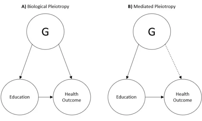
Pleiotropy

These estimates of rG between education and each health outcome provide suggestive

evidence for the presence of pleiotropy, which occurs when one or more genetic variants

influence two or more separate traits or phenotypes (Solovieff et al. 2013). Both Boardman et al.

(2015) and Wedow et al. (2018) also outline a clear distinction between two different types of

pleiotropy, which I adopt here because of its utility for explaining when rG could result in

genetic confounding. Figure 1 can be referenced for a visual representation of the concepts

(18)

10

health outcome have an indirect effect on the health outcome that is mediated through education.

This is defined as mediated pleiotropy (Figure 1B). If measured education completely mediates

the relationship between the pleiotropic variants and the health outcome of interest, rG between

education and that health outcome would not contribute to genetic confounding of the

education-health relationship.

The other possibility is that the genetic variants associated with both education and the

health outcome influence a trait that is a proximate determinant of both education and the health

outcome, such as conscientiousness. That trait would then have a direct effect on both education

and the health outcome. This is defined as biological pleiotropy (Figure 1A). In the case of

biological pleiotropy, because the effect of the genetic variants is not mediated through

education, rG is likely to confound the education-health association. A potential partial solution,

which I test in this paper, is to include polygenic scores for education and the health outcome as

control variables in the model.

Polygenic Scores (PGSs)

An ideal measure to test for genetic confounding would capture all common genetic

influences of education and each health outcome. Because there are no available methods that

can do this, I rely on three separate polygenic scores (PGS) for educational attainment, BMI, and

dep

r

_{ession. A PGS is an additive measure of the effects of individual variants across the genome}

on a phenotype. It can be conceptualized as an additive whole-genome measure of genetic

influence on some outcome (Belsky and Israel 2014; Dudbridge 2013). I include a PGS for

education in all models. I also include PGSs for BMI and depression in models that include BMI

and depression as dependent variables to ensure that as much of the association between

(19)

11

for self-rated health is not available, I include both the PGS for BMI and for depression in all

models that include self-rated health as a dependent variable. This is motivated by the

understanding that self-rated health tends to reflect both physical and mental health (Bailis,

Segall, and Chipperfield 2003).

PGSs are also able to provide some information about the type of pleiotropy that is

occurring. They cannot provide any information about pleiotropy at the level of an individual

genetic variant, but if a PGS is associated with both college degree attainment and health, the

reason for that association is informative for pleiotropy at the level of genome-wide genetic

influence. If the PGS has an indirect effect on health mediated by college degree attainment, this

is evidence for mediated pleiotropy. If the PGS has direct effects on both college degree

attainment and health, this is evidence for biological pleiotropy as previously defined.

While controlling for PGSs does not result in a causal estimate of the effect of a college

degree on health, we still learn a number of things about how genetics factor into the relationship

between college degree attainment and health. If we find evidence for genetic confounding, this

tells us that the observed rG between education and health is at least partly driven by biological

pleiotropy, and we can estimate the proportion of the effect that is confounded. This will be

informative for researchers studying the education-health relationship in the future when making

methodological decisions to account for potential confounders. If we do not find evidence for

genetic confounding, this tells us that the observed rG is driven mostly by mediated pleiotropy,

(20)

12

DATA AND MEASURES

I draw on data collected by the National Longitudinal Study of Adolescent to Adult

Health, hereafter referred to as Add Health (Harris et al. 2009). Add Health is a nationally

representative longitudinal study of adolescents in the United States who were in grades 7-12 in

1994-1995 during Wave I. Data are available for four waves, and data for Wave V of the study

was recently released. Because the Wave V data was released during my analysis, I use data

from Waves I, II and IV. In Wave IV, respondents were between the ages of 24 and 32.

Genotyping was performed in Wave IV, and of the 15,701 participants in Wave IV,

approximately 12,200 were genotyped using two Illumina platforms. Approximately 80% of the

sample were genotyped using the Illumina Omni1-Quad BeadChip and 20% were genotyped

with the Illumina Omni2.5 - Quad BeadChip. Genotyped data were available on 609,130 SNPs

for 9,974 individuals after applying standard quality control procedures. Quality Control

Analysis of Add Health GWAS Data documentation (Highland et al. 2018) provides more

information on the genotyping procedures in Add Health. To account for population

stratification, I restrict my analysis to individuals of European genetic ancestry, bringing the size

of the analytic sample to 5,629 after excluding individuals without valid sampling weights

(Braudt and Harris 2018).

Add Health is an ideal data set to use both because of the available genetic measures in

the data set and because the sample consists of a younger cohort that was representative of the

United States middle- and high-school enrolled population at the time of sampling in 1994-95.

(21)

13

while also providing genetic data on a large portion of its respondents. In addition, in some

respects it has an advantage over other larger datasets with genetic data like the UK Biobank in

that it began with a nationally representative sample of adolescents. While there are other social

science datasets with genetic data that are nationally representative like the Health and

Retirement Study, Add Health provides the opportunity to examine a cohort who has more

recently experienced their educational attainment. Given evidence that genetic effects are

conditional on the environmental context (Tropf et al. 2017), it is important to assess genetic

confounding for different cohorts who experience their educational environments in different

time periods. It is important to note that while Add Health was designed to be nationally

representative, my analysis is restricted to individuals with European genetic ancestry. Therefore,

the results cannot be generalized to populations with non-European genetic ancestry.

I measure educational attainment in Wave IV in order to capture the highest level of

education that respondents have attained at the age of 24-32. I use receipt of college degree

rather than years of education in order to facilitate the propensity score analysis described below.

While neither parameterization is likely to perfectly represent the functional form of the

relationship between education and health, there is some evidence that college education is

uniquely important for health (Montez et al. 2012).

Because Wave V data on the full sample were not available at the time of this analysis, I

also measure the three health outcomes of interest at Wave IV. While it would be ideal for the

measurement of education to occur at a time point before the health measurements, most of the

respondents will not have finished their educations at Wave III. I use the constructed measure of

body mass index (BMI) as a continuous variable. This was calculated using the height and

(22)

14

and BMI calculated from those measures, have been shown to be highly reliable in Add Health

(Hussey et al. 2015). To measure self-rated health, respondents were asked “In general, how is

your health?” and were able to choose between “excellent”, “very good”, “good”, “fair”, and

“poor”. I treat self-rated health as an ordinal variable.

To measure depression, I use a measurement model with four indicators drawn from the

Center for Epidemiological Studies Depression Scale (CES-D Scale) (Radloff 1977). The subset

of items I am using were originally part of a measurement model proposed and validated by

Perreira et al. which, in line with measurement theory, is composed of only the effect indicators

in the original scale while excluding any causal indicators or outcomes of depression (Perreira et

al. 2005). Because this is a rare case in which a measurement model has already been tested and

validated in the dataset I am using, it makes sense to begin with this as my initial specification.

Figure 2 is the path diagram representing the model. Respondents were asked, “How often was

the following true during the past seven days?” and then given the following four prompts. “You

could not shake off the blues, even with help from your family and your friends.” “You felt

depressed.” “You felt happy.” “You felt sad.” Respondents were given a “0” if they chose “never

or rarely”, a “1” if they chose “sometimes” a “2” if they chose “a lot of the time”, and a “3” if

they chose “most of the time or all of the time”. I treat each of these indicators as an ordered

categorical variable.

Because genotype is determined at birth and PGSs are a summary genetic measure, it

may seem unnecessary to include control variables if we are interested in estimating effects of

the PGSs. However, the effects of PGSs are known to be confounded by family background

because parents both transmit their genetics to their children and influence their educational

(23)

15

background, the effect of genetic confounding could be overestimated. Furthermore, a secondary

aim of this study is to investigate genetic confounding that would not be captured by variables

that researchers commonly have access to in large social science surveys.

To accomplish both goals, I estimate two sets of models. The first set of models includes

covariates only meant to control for the confounding effects of family background at Wave I. I

do not include individual characteristics of the adolescents in this set of models because they

may mediate the effects of the PGSs. In the second set of models I attempt to control for many

potential confounders of the relationship between college degree attainment and health in the

Wave I and II data.

1

_{Because Lawrence (2017) previously attempted a similar strategy to account}

for selection into college degree attainment in Add Health, the first set of models includes the

following subset of the variables used by Lawrence.

Parents’ education is measured using an average of resident parent years of education.

When data do not exist for both parents, I use the education level of one parent. Parent

occupation is measured using two binary indicators of whether the resident mother and father

each have professional jobs. As a measure of family income, I follow Lawrence (2017) and use a

categorical income-to-needs ratio variable. This ratio is calculated by dividing the household

income by the poverty threshold in 1994 for the adolescent’s household size. I create a separate

missing category for this variable because 18% of the respondents have missing information.

Other household level controls at Wave 1 include whether the respondent had health insurance,

whether the parent interviewed received public assistance, whether there was a smoker in the

household, and the household size. Controls for parent health behaviors include whether the

1_{While many of these covariates likely confound the relationship between college degree attainment and health, they} also likely mediate the effect of the PGSs on college degree attainment and health respectively. I therefore do not include all covariates used by Lawrence (2017) in the first set of models because it would result in the

(24)

16

parent smoked and the frequency of parent heavy drinking. Age, sex, and whether the respondent

was born in the United States are also included as control variables in all models.

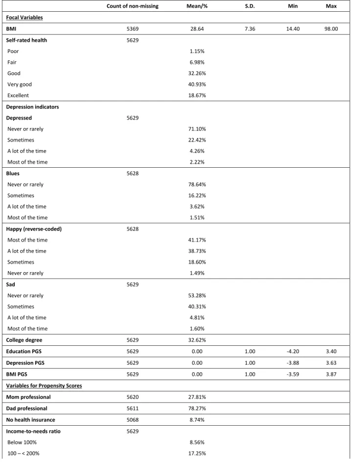
As a control variable for the second set of models, I estimated propensity scores using the

list of variables in Table 1 under the “variables for propensity scores” heading, which includes

the variables described above. These are the same variables included in Lawrence’s (2017)

analysis. To handle missing data, ten datasets were imputed using the data imputation command

in Mplus version 8.2.

To measure genetic contributions to the outcomes of interest in this study, I rely on three

publicly available PGSs from Add Health for educational attainment, BMI, and major depressive

disorder, respectively (Braudt and Harris 2018; Lee et al. 2018; Locke et al. 2015; Wray et al.

2018). Each polygenic score represents the cumulative additive genetic influence on the

phenotype of interest (Belsky and Israel 2014). The PGS for an individual

𝑖

is calculated as:

𝑃𝐺𝑆 =

𝛽 𝑆𝑁𝑃

where,

𝑆𝑁𝑃

is the number of alleles of the

𝑗

SNP for the

𝑖

individual and

𝛽

is the estimated

association between SNP

𝑗

and the phenotype as reported in the summary statistics for a GWAS

of that phenotype based on an independent sample. The PGSs are then standardized to have a

mean of 0 and a standard deviation of 1. For more information on the calculation of the PGSs

used in this study, see Braudt and Harris (Braudt and Harris 2018).

Even in samples restricted on ancestry, population stratification can still create spurious

associations between PGSs and outcomes (Price et al. 2006). This occurs because ancestral

differences within populations may be associated with but causally unrelated to outcomes of

(25)

17

of PGSs. A common method for addressing this, which I use here, is to regress the original PGSs

scores on the first ten ancestry-specific principal components of the genetic data, save the

(26)

18

METHODS

While past studies have estimated non-zero rG between education and these health

outcomes in other datasets, it is preferable to provide evidence of this in Add Health before

moving on to more complicated analyses. I do this by estimating bivariate correlations between

all variables of primary interest in the analysis, which include the PGSs, college degree

attainment, and the three health outcomes.

2

I begin the analysis examining the relationship between receipt of a college degree and

depression with the estimation of the confirmatory factor analysis model (measurement model)

for depression described above and illustrated in Figure 2. “You felt depressed” is used as the

scaling indicator.

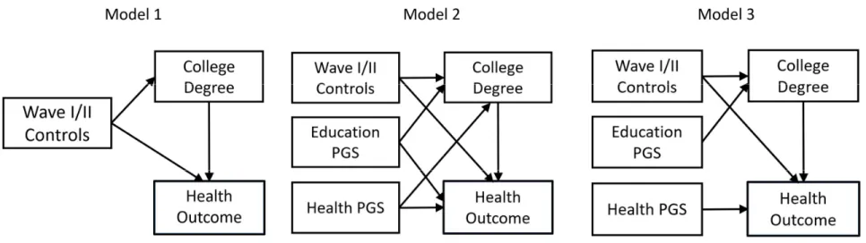
I then estimate a series of structural equation models (SEMs). The general path diagrams

representing these models are in Figure 3. The purpose of each is to test whether genetics

confound the relationship between receipt of a college degree and each of the three health

outcomes (depression, BMI

3

_{, and self-rated health). The right side of each diagram includes}

variables measured in Wave 4 and depicts the relationship between education and the health

outcome of interest. There are a few reasons why SEM is preferred for this analysis. For one,

depression is best modeled as a latent variable to control for measurement error, which is easily

done in an SEM framework. Because the depression models are overidentified, I am also able to

take advantage of various model fit statistics. Furthermore, the tradition of presenting path

2_{I declare college degree attainment and self-rated health to be categorical variables before estimating the}

correlations.

(27)

19

diagrams with SEM analyses, which I do here, helps with interpretation of the model results. The

models that do not include the latent measure of depression are fully recursive, so the results

would be no different if they were estimated one equation at a time using standard regression

models. Finally, as explained below, I exploit a feature of structural equation modeling software

used for mediation analysis to formally test for a confounding effect.

In the first round of models, the controls on the left sides of the diagrams are possible

confounders of the effects of the PGS and the reason for including them is discussed above. All

control variables are entered separately in the models and can correlate but are represented in the

path diagrams as one observed variable for parsimony.

In the second round of models, I replace the smaller set of control variables with a

propensity score to represent the joint confounding effects of all covariates that were included in

the first round of models plus the variables under the heading “variables for propensity scores” in

Table 1. Lawrence (2017) applies propensity scores estimated using these same covariates to

account for selection into a college degree, and she acknowledges in her limitations section that

she was not able to account for genetic factors. Some of the variables used to estimate the

propensity scores will likely mediate the influence of the PGSs in this analysis. For example,

Wave I measures of the health outcomes are included in the estimation of the propensity scores.

However, the purpose of the propensity score analysis is to see whether any evidence of genetic

confounding remains after controlling for a wide range of possible confounders measured at

Waves I and II. This is therefore a conservative test of genetic confounding, as many of the

covariates included in the propensity score model will inadvertently capture some genetic

(28)

20

regression model of the receipt of a college degree on relevant variables listed in Table 1 and

saving the propensity scores. This was done separately for each of the 10 imputed datasets.

The direct effects of the education PGS on the health outcome and the direct effect of the

relevant health PGS on receipt of a college degree are the primary coefficients of interest for this

analysis. For example, there is likely to be a significant non-zero direct effect of the education

polygenic score on receipt of a college degree. This would not indicate genetic confounding. If

this same polygenic score also influenced depression however, this would then make education

linked genetics a possible confounder in the relationship between receipt of a college degree and

depression. We would also expect the PGS for BMI to have a significant non-zero direct effect

on BMI, but if it has a significant non-zero direct effect on receipt of a college degree, this

indicates possible genetic confounding.

For each health outcome under consideration, I fit models using two different

specifications. Path diagrams for each specification are in Figure 3 where they are labeled as

Model 1 and Model 2. The equation predicting the health outcome in Model 1 can be understood

as a regression of the health outcome on receipt of a college degree with controls for observed

covariates, no PGSs are included. The effect of a college degree on health in this model will be

treated as a baseline for comparison with the effects from the second model.

Model 2 adds direct paths from both PGSs to both education and the health outcome,

which is the test of genetic confounding. If one PGS has a direct effect on both education and the

health outcome, it confounds the association. This would provide evidence for genetic

confounding. Model 3 includes PGSs for both education and the health outcome but assumes that

each polygenic score only has a direct effect on the outcome it is optimized to predict. For

(29)

21

depression, but not to education. Likewise, it includes a direct path from the PGS for education

to college degree, but not to depression.

To formally test for genetic confounding, I exploit a common feature of structural

equation modeling programs that is commonly used for mediation analysis. To test for mediation

in structural equation models, it is common to estimate an indirect effect by taking the product of

the direct effects that lie along the path of meditation (Bollen 1989). Variability of the indirect

effect can then be estimated using the delta method or bootstrap methods (Bollen and Stine 1990;

Sobel 1982). It is well known that mediation and confounding are statistically equivalent, and

that the only way to distinguish between the two processes is by using theoretical knowledge

about the causal ordering of variables (MacKinnon, Krull, and Lockwood 2000). Therefore, I test

for the significance of the confounding effect by testing for the significance of an indirect effect

of college degree attainment on health in an “incorrect” model where the PGSs serve as

mediators rather than confounders. Each equation in this model includes as covariates those

control variables that are present in the corresponding “correct” model.

For symmetry between the analyses using observed covariates and propensity scores, I

use the propensity score as a covariate to adjust the models described above. While this is a

common approach in the literature, some have discouraged this use of the propensity score

because it assumes a linear relationship between the propensity score, the treatment, and the

outcome (Austin 2011). As a robustness check, I use the propensity score to calculate inverse

probability of treatment weights (IPTW) to weight the sample so that it is balanced on the

(30)

22

effect of a college degree on the health outcomes.

4

_{I can then test for genetic confounding in}

cases where it remains after including the propensity score as a covariate in the model.

Estimation

All analyses were performed in Mplus version 8.2. For all depression and BMI models, I

first estimated them using a robust weighted least squares estimator using a diagonal weight

matrix (WLSMV in Mplus) to handle both the categorical nature of the depression indicators and

the college degree variable and because this estimation method provides a wide array of fit

statistics. However, when using WLSMV in models with categorical mediators, the continuous

latent response variable rather than the categorical itself is used as the covariate in the regression

of the outcome on the mediator. Because college degree is a categorical mediator in all models,

this would affect the interpretability of the college degree coefficient. In models estimated using

WLSMV, the college degree coefficient gives the expected change in the outcome that

corresponds to a one-unit change in a latent variable underlying the binary college degree

variable. This coefficient is not directly interpretable as the effect of a college degree. To solve

this problem, I also estimated all depression and BMI models using maximum likelihood with

robust standard errors (MLR in Mplus), which uses the observed mediator as the covariate and

allows for the direct interpretation of the effect of a college degree.

For models predicting self-rated health, I estimate each equation of the model separately

which is reasonable because the model is fully recursive. I use MLR to estimate the equation

predicting receipt of a college degree as was done in other models, but I use WLSMV to estimate

the equation predicting self-rated health. This is done because self-rated health is an ordinal

4_{Individuals with propensity scores equal to zero or one were excluded from these analyses. Individuals with}

(31)

23

variable and WLSMV in Mplus provides y-standardized coefficients. Y-standardizing the

coefficients allows for an interpretation of coefficients that is analogous to linear regression. It

also allows for the comparison of the effect of a college degree across different self-rated health

models, as this method of interpretation is not affected by the rescaling problem that comes with

comparing odds ratios across different nonlinear probability models (Breen, Karlson, and Holm

2018). However, I cannot estimate the full model using WLSMV because of the problems

discussed above.

5

_{All analyses account for the complex sampling design of Add Health through}

sampling weights, stratification, and clustering.

5_{I used a binary measure of education to facilitate the creation of propensity scores, but it is important to note that}

(32)

24

RESULTS

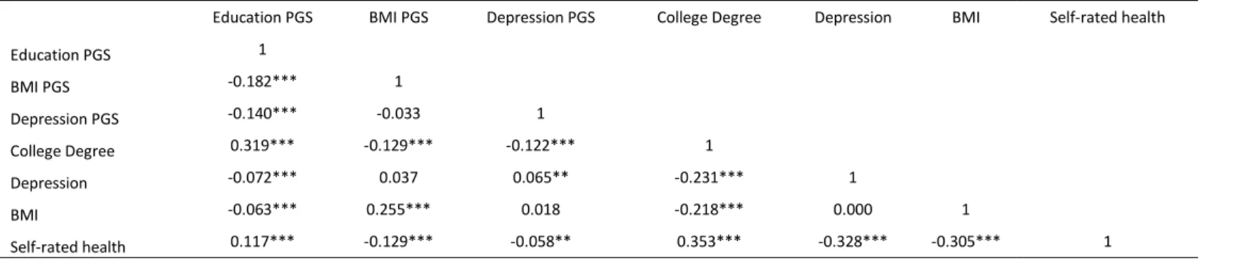
Beginning with the indirect tests of rG, we can see in Table 2 that the educational

attainment PGS correlates with the BMI PGS at -0.182 and the depression PGS at -0.140. These

are relatively weak in magnitude but statistically significant. This suggests that on average, the

genetic variants associated positively with educational attainment tend to be negatively

associated with BMI and depression, at least for the variants captured in the PGS. On the other

hand, the correlation between the PGS for BMI and the PGS for depression is -0.033 and not

statistically significant, suggesting that there is no clear relationship between the genetic variants

associated with BMI and depression. While there may be relationships between individual

variants captured by the PGSs, a correlation between the two PGSs would not necessarily show

this.

We can also examine the correlations between the PGSs and relevant outcomes in the

same table. Starting with the relationships between the health PGSs and college degree

attainment, the BMI PGS and college degree attainment are significantly correlated at -0.129 and

the depression PGS and college degree attainment are significantly corelated -0.122. The

education PGS is also significantly correlated at -0.072 with depression, -0.063 with BMI, and

0.117 with self-rated health. Taken together with the past studies of rG previously reviewed,

these results provide evidence for rG between educational attainment and these three health

outcomes in the Add Health cohort. While the correlations estimated here are modest, they are an

(33)

25

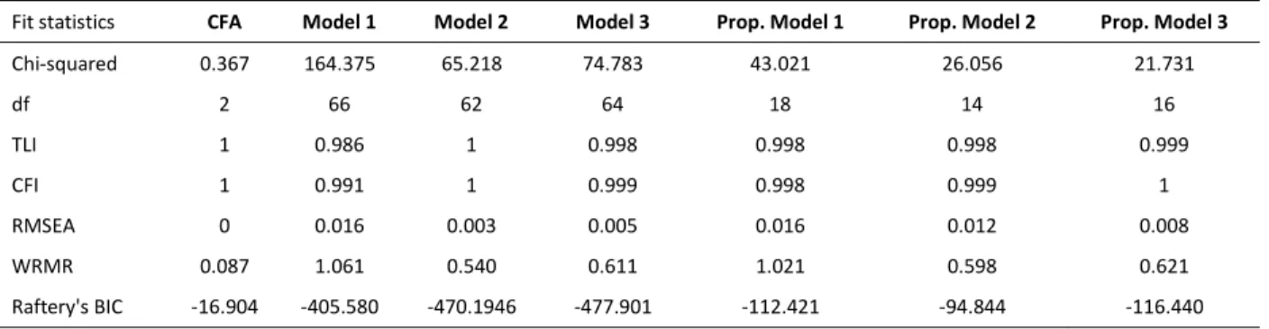
The first model to be fit is a confirmatory factor analysis of depression as outlined above.

As shown in Table 3, the model fits the data very well. The TLI and CFI are both equal to 1, and

the RMSEA is 0. The chi-squared statistic

6

_{is small and the BIC (Bollen et al. 2014; Raftery}

1995) is around -17. The R

2

_{values of the indicators range from .519 to .879, which means that}

the latent variable of depression is explaining a relatively large amount of the variance in the

underlying indicators. After determining that the measurement model fits well, we can now turn

to the fit of the structural equation models predicting depression.

The main paths of interest in this model are the direct paths from the polygenic scores to

education and depression, so each specification of the model sets some of these paths to be

estimated and some others to be zero. The columns in Table 3 are labeled according to the model

specifications pictured in Figure 3. Model 1, which constrains the direct effects of both PGSs on

both college degree and depression to be zero, has the worst fit according to all the fit statistics

presented. Model 2, which frees all paths that were constrained in Model 1, has a fit that is

almost indistinguishable from Model 3, which constrains the effect of the depression PGS on

college degree and the effect of the education PGS on depression to zero. This means that the

structure of Model 3 is assuming that there is no direct effect of the polygenic score for

education on depression, and there is no direct effect of the polygenic score for depression on

education. Model 2 however, is assuming that the PGSs operate as confounders, having direct

effects on both college degree attainment and depression. Because the fit statistics between

Model 2 and Model 3 are very similar, examining the regression coefficients of the models

6_{All fit statistics reported for the depression models are means averaged over the ten imputed datasets. For this}

(34)

26

provides more information to judge whether genetic factors are a possible confounder of the

relationship.

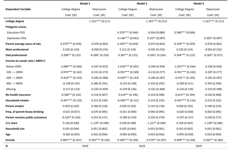
The results for the models predicting depression are presented in Table 4. In Model 1,

which does not include PGSs, having a college degree is associated with a 1.352 unit decrease in

depression. In Model 2, both PGSs are included as potential confounders of the relationship, as a

confounder should have a significant direct effect on both education and depression. While the

education PGS only has a direct effect on college degree attainment, the depression PGS has a

significant direct effect on both college degree attainment and depression, providing some

evidence for genetic confounding by the depression PGS. If the PGSs were confounders of the

association, a failure to control for them would result in a biased estimate of the effect of

education and we would therefore expect the effect estimate to change as they were added to the

model. In Model 2, the college degree coefficient is associated with a 1.301 unit decrease in

depression, which is a change of about 4% from model 1. Using the method described above to

estimate the total indirect effect, the estimate of the confounded effect was not determined to be

statistically significant (p = 0.126). However, a small specific indirect effect through the

depression PGS was detected (β = -0.035; p = 0.046), which suggests that the depression PGS

could operate as a partial confounder of the relationship between college degree attainment and

depression. Overall, the evidence for genetic confounding here is relatively weak, as is the

evidence for biological pleiotropy as an explanation for rG. However, failing to control for PGSs

in this context could result in a slight overestimate of the effect of a college degree on

depression. In the relationship between college degree attainment and depression, observed

college degree attainment also mediates the relationship between the education PGS and

(35)

27

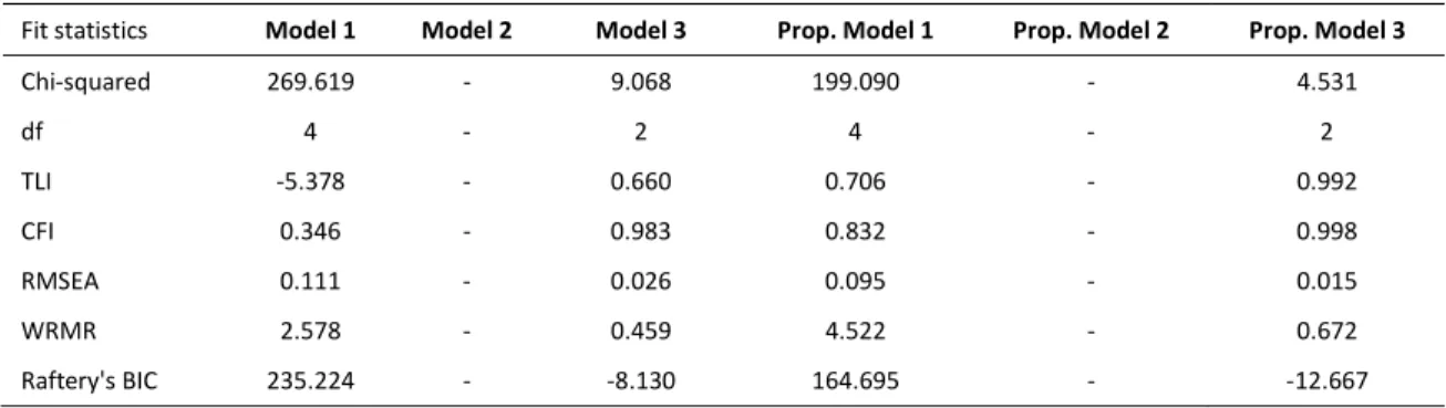
For the models focused on the relationship between college degree attainment and BMI

and between college degree attainment and self-rated health, Model 2 is exactly identified and so

it has no fit statistics. However, it is the saturated model that is automatically compared with

Models 1 and 3 through their fit statistics. The fit statistics for the BMI models are in Table 5.

Model 1, which constrains all the effects of the PGSs, has a terrible fit. Model 3, which freely

estimates the effects of the PGSs only on their corresponding phenotypes, has a much better fit,

but still has room for improvement, especially on the TLI.

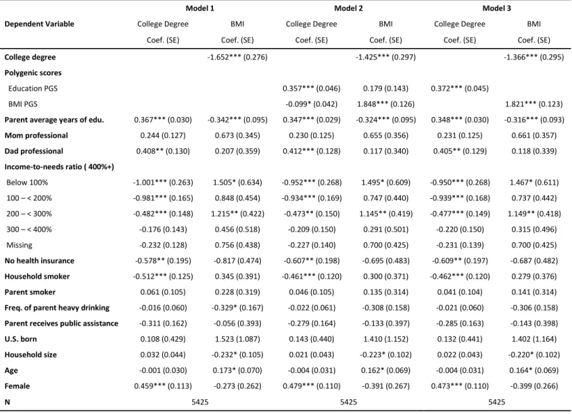
The regression results from the models predicting BMI are displayed in Table 6. After

controlling for the education PGS and the other observed covariates in Model 2, the BMI PGS

has a significant direct effect on both college degree attainment and BMI. Furthermore, we can

compare the regression coefficients on college degree between Model 1 and Model 2. In Model 1

graduation from college is associated with a decrease in BMI of 1.652 units, while in Model 2 it

is associated with a decrease in BMI of 1.425 units. The absolute value of the coefficient

decreases by about 14% (p = 0.008). This provides evidence for genetic confounding, as the

estimated effect of education weakens significantly after controlling for the PGS. The substantial

statistically significant decrease in the effect of a college degree on BMI between the two

models, the significant direct effect of the BMI PGS on college degree attainment and BMI in

Model 2, and the less than ideal fit of Models 1 and 3 provide evidence for genetic confounding

of the relationship between college degree attainment and BMI. While we find evidence for

genetic confounding, and therefore biological pleiotropy likely partially contributes to the rG

between education and BMI, we can also see that the PGS for education has an indirect effect on

(36)

28

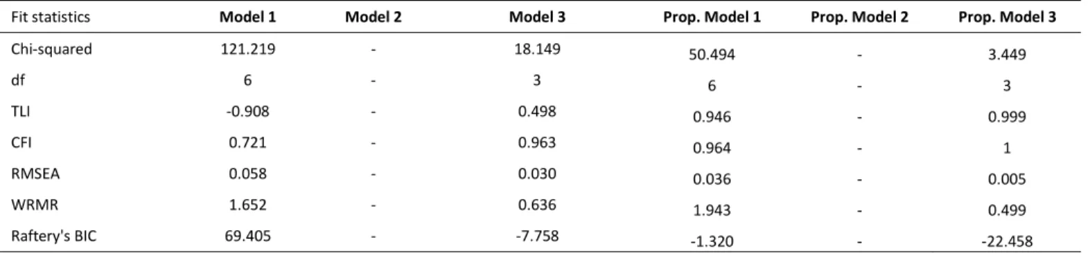
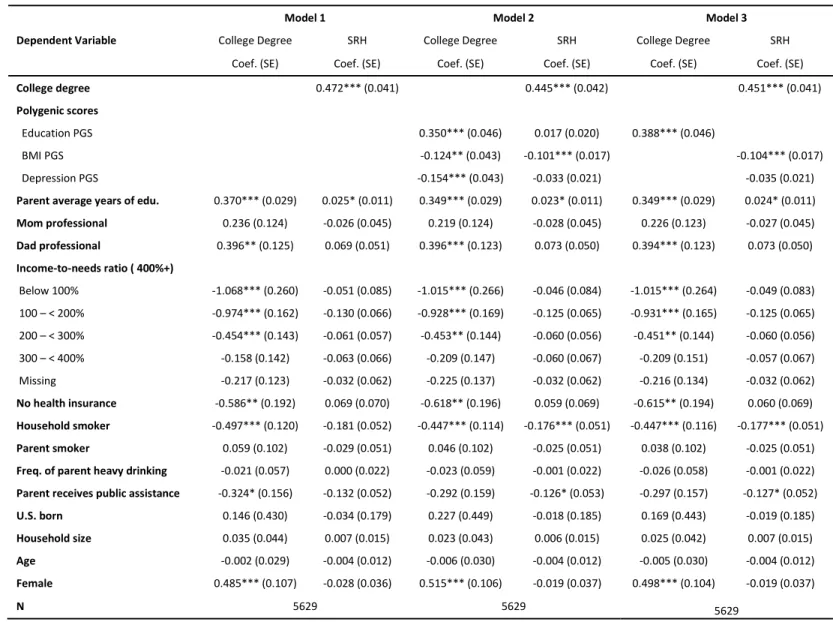
Turning to the fit statistics for the self-rated health models in Table 7, we can observe

that they are patterned similarly to the fit statistics for the BMI models. Model 1 again has a

terrible fit, and Model 3 is better but shows room for improvement. This provides suggestive

evidence for genetic confounding, but the regression estimates provide additional evidence. In

Model 1 predicting self-rated health (Table 8), graduating from college is associated with a 0.449

(

0.472 𝜎

⁄

∗

)

standard deviation increase in self-rated health. In Model 2, after controlling for the

education, BMI, and depression PGSs, graduating from college is associated with a 0.421

(

0.445 𝜎

⁄

∗

)

standard deviation increase in self-rated health.

Given that the model predicting self-rated health is an ordinal probit, we cannot directly

calculate the percent decrease in the effect of education on self-rated health from the coefficients

as we move from Model 1 to Model 2 in Table 6. This approach is inappropriate in nonlinear

probability models such as ordinal logistic regression because adding additional variables to

these models will affect both the residual variance of the model and the true effects of the

variables in the model. The change in the coefficient captures both effects, so it does not allow us

to distinguish between true confounding and a change in the residual variance. This is not a

problem in linear regression because the residual variance is estimated separately (Breen et al.

2018). In order to retrieve unbiased estimates of genetic confounding, I divide the college degree

coefficient by the estimated standard deviation of the continuous latent variable underlying

self-rated health (Breen et al. 2018).

Using the product coefficient method described above, about 6% (p < 0.001) of the effect

of college degree attainment on self-rated health is confounded by PGSs for education, BMI, and

depression. In Model 2, the PGS for BMI also has a statistically significant direct effect on both

(37)

29

is smaller than in the college degree and BMI relationship, failing to control for common genetic

factors results in a small overestimate of the effect of a college degree on self-rated health. As in

the models predicting depression and BMI, we also observe evidence for mediated pleiotropy in

the relationship between college degree attainment and self-rated health, as the education PGS

has an indirect effect on self-rated health that is mediated through observed education.

The above analyses are informative because they only include additional controls that

represent the respondent’s family background in Wave I. They are unlikely to mediate the effects

of the PGSs in this case. However, given the rich information available in Add Health and in

many other social science surveys, one might wonder whether the evidence for genetic

confounding presented above remains after controlling for variables that may inadvertently

capture genetic effects. This question motivated the analyses using propensity scores reviewed

below.

Table 3 also includes the fit statistics from the three depression models that include a

propensity score. The only difference between these models and the previous three depression

models is that a propensity score, saved from a probit regression of college degree attainment on

the covariates in Table 1, replaces the covariates in the previous models.

7

_{Unlike the first round}

of depression models, Model 1, which constrains the effects of the PGSs to zero, is no longer

clearly the worst fitting model, and all three of the models seem to fit well. However, if one

model were to be chosen based on the fit statistics alone, Model 3 seems to be the best fitting

model. As a reminder, Model 2 allowed all coefficients to be freely estimated, while Model 3

constrained the effect of the education PGS on depression and the effect of the depression PGS

(38)

30

on college degree attainment to be zero. This provides some evidence that the small confounding

effect of the depression PGS might have been blocked by the propensity score.

We can also examine the regression coefficients for these models in Table 9. The first

thing to notice is that the depression PGS no longer has a significant direct effect on college

degree attainment or depression in Model 2. In addition, graduating from college is associated

with a .632 unit decrease in depression in Model 1, which is a 53% decrease from the original

specification of Model 1 that did not include a propensity score. This is a much larger decrease

than occurred after including the PGSs in the original models, suggesting that the propensity

score is accounting for more confounding than were the PGSs. After controlling for the PGSs in

the propensity score models, the college degree coefficient still declines by about 2% from

Model 1 to Model 2, but neither the total indirect effect nor either of the specific indirect effects

estimated using the product method are statistically significant. When we also consider the lack

of differences in fit across models and the non-significant direct effect of the depression PGS on

college degree attainment and depression in Model 2, we can conclude that any small

confounding effect of the depression PGS was blocked by the propensity score.

For the propensity score models predicting BMI, Model 1 has a noticeably worse fit than

Model 3, but Model 3 fits well and only has a small amount of room for improvement (Table 5).

This is suggestive evidence that the propensity score may be capturing at least some of the

genetic confounding effect from the first series of BMI models. The estimated effect of a college

degree is also much smaller in Model 1 compared to the same model without the propensity

score. In Table 10, graduating from college is associated with a 1.071 unit decrease in BMI,

which is a 35% absolute decrease from the same coefficient reported in Table 6. As in the

(39)

31

than the PGSs alone. In Model 2, the effect of the BMI PGS on college degree attainment is no

longer significant like it was in Model 2 without the propensity score and graduating from

college is associated with a 0.964 unit decrease in BMI. Moving from Model 1 to Model 2 in

Table 8, the coefficient on college degree decreases by about 10%. While this change might

seem relatively large, the total indirect effect estimated through the product method is not

statistically significant (p = 0.217). As with depression, it appears as if controlling for the

propensity score blocks the genetic confounding effect that was found in the previous round of

models.

The fit of the models predicting self-rated health with propensity scores is like that of the

BMI models with propensity scores, in that Model 3 fits very well, while Model 1 does not fit as

well (Table 7). Again, this suggests that the propensity score may be blocking at least a portion

of the previously identified genetic confounding. In Table 11, we can see that the y-standardized

effect of a college degree on self-rated health decreased from 0.449 (