School of Computing and IT, Makerere University, Kampala, Uganda; [email protected] 2 AI Lab, Makerere University, Kampala, Uganda; [email protected]
* Correspondence: [email protected]
Abstract:Rapid increase in digital data coupled with advances in deep learning algorithms is opening unprecedented opportunities for incorporating multiple data sources for modeling spatial dynamics of human infectious diseases. We used Convolutional Neural Networks (CNN) in conjunction with satellite imagery-based urban housing and socio-economic data to predict disease density in a developing country setting. We explored both single (uni) and multiple input (multimodality) network architectures for this purpose. We achieved maximum test set accuracy of 81.6 per cent using a single input CNN model built with one convolutional layer and trained using housing image data. However, this fairly good performance was biased in favor of specific disease density classes due to an unbalanced data set despite our use of methods to address the problem. These results suggest CNN are promising for modeling spatial dynamics of human infectious diseases, especially in a developing country setting. Urban housing signals extracted from satellite imagery seem suitable for this purpose, under the same context.
Keywords:Convolutional Networks; satellite imagery; predictive modeling; disease density; urban housing; developing country
1. Introduction
Data-intensive computing (big data in concert with advanced machine learning) is projected to play an important role in shaping the future of research in public health generally and computational epidemiology in particular. Several application areas are earmarked in which big data together with deep learning are expected to make significant impact including disease surveillance, medical imaging, medical informatics, bio-informatics, and pervasive sensing [1], [2], and [3]. Current research in this area is however, mostly focused on applications in disease surveillance. For example, Garimella et al. [4] used deep neural networks (DNN) and images posted on social media to infer national health statistics on lifestyle diseases. Ong et al. [5] applied deep recurrent neural networks (DRNN) to predict concentration of particulate matter using textual environmental monitoring data. RNN were also used by Dernoncourt et al. [6] to de-identify patients in textual medical records. Kendra et al. [7] used DNN to analyze and determine discourse on health-related topics using text-based social media content. DNN (skip-gram) were used by Zou et al. [8] on social media data (text) to detect and quantify cases of infectious intestinal diseases. Mobile phone meta-data were used as input data to a Convolutional Neural Network (CNN) [9] and a combination of CNN with Support Vector Machines (SVM) to predict demographic characteristics (age and gender) by Felbo et al. [10]. Lastly, Deep Bayesian Networks (DBN), especially Social Restricted Boltzmann Machines (SRBM) were proposed by Phan et al. [11] for understanding human behavior in health social networks. Communication data consisting of text was used as input to the model.
As can be seen from the example works cited above, research in potential applications of deep learning for disease surveillance is dominated by use of data extracted from social media and other online sources. While an important source that has demonstrated great promise, their applicability in a study may be limited to geographical regions where social media and the Internet are widely used as
source of health information. For other regions and for population-based risk-related investigations however, alternative sources of digital data must be explored for disease surveillance within the context of digital epidemiology.
In this article we explore opportunities afforded by recent advances in deep learning (DL) for studying disease dynamics using alternative data sources than social media. Specifically, we use Convolutional Neural Networks (CNN) together with satellite imagery-based housing and socio-economic data to predict disease density in a developing country urban setting. Indoor overcrowding (for which we use housing crowding as proxy) and socio-economic well-being are the most important risk factors for our case study disease i.e.Tuberculosis(TB), especially for urban settlements in the study area [12]. TB is a leading cause of death among HIV/AIDS patients in Uganda [13] [14], our study area. The advantage of using DL over conventional machine learning methods is that features used for analysis and prediction are learned automatically from raw input data, thus saving model development complexity. Secondly, DL network architectures especially CNN support simultaneous data input and processing, which is necessary for prediction tasks based on multiple concurrent variables. The contribution of this work is two-fold as follows,
1. We propose a CNN model for predicting disease density. The model takes as input, data from single (or multiple concurrent) source(s) and outputs an estimate of per ca-pita disease density for a geographical region of interest. We instantiated the model by using as input, image data for urban housing and poverty to predict TB in a developing country setting. Our model may be used for infectious disease surveillance and for public health intervention planning.
2. We have established the relative suitability of housing crowding signals extracted from satellite imagery for the purpose of predicting disease density using CNN in a developing country urban setting. This result broadens currently available sources of data for investigating phenomena associated with infectious diseases using machine learning techniques.
The remainder of this paper is structured as follows. Results, discussion, materials and methods are presented in Sections2,3, and4, respectively. We draw conclusions in section5.
2. Experimental Results
The evaluation of our model was done in two phases. First, we evaluated all candidate network architectures for our proposed CNN model on the basis of predictive accuracy. The purpose was to identify architectures that were optimal for the nature and size of our data set from among the single-(unimodality) and multiple (multimodality) input architectures. The top three candidates with highest accuracy were then selected for further optimization using a set of hyperparameters to build a robust CNN model for predicting disease density. Results of evaluating various architectures on prediction accuracy are shown in Table1and2, respectively.
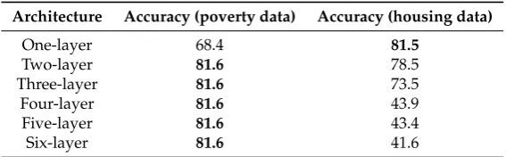
Table 1.Test set accuracy (%) for single input CNN models.
Architecture Accuracy (poverty data) Accuracy (housing data)
One-layer 68.4 81.5
Two-layer 81.6 78.5
Three-layer 81.6 73.5
Four-layer 81.6 43.9
Five-layer 81.6 43.4
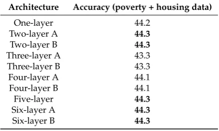
Three-layer A 43.3
Three-layer B 43.3
Four-layer A 44.1
Four-layer B 44.1
Five-layer 44.3
Six-layer A 44.3
Six-layer B 44.3
The results are also summarized using bar plots in Figure1,2, and3, respectively.
Figure 1.Bar plot showing overall accuracy for single-input CNN models trained on poverty data.
Figure 2.Bar plot showing overall accuracy for single-input CNN models trained on housing data.
Figure 3.Bar plot showing prediction accuracy for multi-input CNN models trained on concurrent input of housing and poverty data.
cent, respectively, among the single input architectures (see bold text results in Table1. On the other hand, the 2-, 5-, and 6-layer architectures performed best all at 44.3 per cent among the multi-input architectures, Table2. However, accuracy for the best multiple input model at 44.3 per cent was far worse than that for the best single input model at 81.6 per cent. For this reason we selected for further optimization the 1-layer single input model trained on housing data and the 2- and 3-layer models trained on poverty data, based on the principle of parsimony. Our objective here was to squeeze further improvement in predictive accuracy from the three selected architectures.
Hyperparameters we considered for optimizing our three best-performing candidate models include convolution type, kernel size, and filter count. These are some of the important hyperparameters that were not optimized in previous experiments. Further experiments were thus carried out to optimize these trainable parameters on the three candidate models. For convolution type, we adopted the use of depthwise separable convolutions [15] instead of standard convolutions. The former architecture "separates the learning of spatial and channel-wise features" [16]. The result is a lightweight, faster, and more accurate model on the task at hand. Depthwise separable convolutions are also said to learn better representations using small training sets. Three optimization experiments based on depthwise separable convolutions were carried out for each of the three selected models for a total of nine experiments. The results showed zero to negligible improvement in predictive performance for all models, see Table3.
Table 3.Accuracy (%) on Standard and Depth-wise separable convolutions.
Architecture Standard Depthwise Gain (%)
One-layer 81.5 81.6 0.1
Two-layer 81.6 81.6 0
Three-layer 81.6 81.6 0
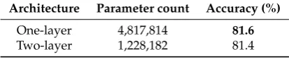
We also wanted to know if larger kernel size and filter count would lead to improvement in prediction accuracy. So we tried out a kernel size of 7 x 7 (instead of a 3 x 3 one used in previous experiments) and filter count of 128 (instead of 64) on the 1- and 2-layer architectures (selected for their simplicity). Recall that other important hyperparameters such as learning rate, learning rate scheduling, weight decay, etc were already being applied to the previous training processes, so their values were simply maintained throughout these optimization experiments. Three experiments were completed per architecture based on this new hyperparameter configuration for a total of six experiments. Average results are reported in Table4.
Table 4.Test accuracy (%) for larger kernel size and filter count for two overall best models.
Architecture Parameter count Accuracy (%)
One-layer 4,817,814 81.6
Two-layer 1,228,182 81.4
Figure 4. Confusion matrix plot for our overall best model. Key: 0 - high disease density, 1 - low disease density, 2 - moderate disease density.
Figure 5.Area under receiver operating characteristic curve (AU-ROC) plot for our overall best model. Key: 0 - high disease density, 1 - low disease density, and 2 - medium disease density.
Table 5.Precision, recall and f1-score values for our overall best model.
Disease class Precision Recall F1-Score
High disease density 0.83 0.58 0.69 Moderate disease density 0.68 0.84 0.75 Low disease density 0.87 0.78 0.83
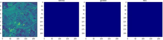
Figure 6. Visualizing features used in predicting class: high disease density. Case where learned features were visually perceptible.
Figure 7. Visualizing features used in predicting class: high disease density. Case where learned features were visually imperceptible.
Figure 8.Visualizing features used in predicting class: moderate disease density. Case where learned features were visually perceptible.
Figure 9.Visualizing features used in predicting class: moderate disease density. Case where learned features were visually imperceptible.
Figure 11. Visualizing features used in predicting class: low disease density. Case where learned features were visually imperceptible.
In general, it is clear from our visualizations of class activation maps (columns 2, 3, and 4) in Figures6,8, and10that our model is learning (and using), more so correctly, features associated with housing to make classification decisions.
3. Discussion
The goal of this work was to develop a CNN model for predicting disease density. The primary model objective was therefore, prediction accuracy followed by transparency. To attain this goal we needed to,
• Identify a CNN network architecture that was optimal for the nature and size of data set we had, • Tune a set of hyperparameters to build a model with high predictive accuracy and ability to
generalize well on data previously not seen by the model.
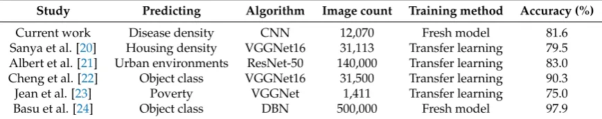
For the first task we evaluated an architecture search space consisting of 10, 2-branch multi-input and 6, single-input architectures up to 6 layers deep. We found that a 1-layer single-input architecture constructed with a depthwise separable convolution is most optimal when trained on housing satellite image data. A model built using this architecture gave the highest test set accuracy of 81.6 per cent using hyperparameter values and/or methods specified in Table12, in addition to using a kernel size of 3 x 3 and filter count of 64. The model also performed well in terms of predicting individual classes (Figure4), exactness (precision), and completeness (recall), Table5. The accuracy attained by our model, more over with a small training set, falls within range of current state-of-the-art results obtained elsewhere on similar data sets. For example, [20], [21], [22], [23], and [24] all worked with satellite imagery data and CNN (or other deep learning framework) for different classification problems and obtained accuracy between 75 and 97 per cent (Table6).
Table 6.Classification accuracy on different satellite scene image data sets.
Study Predicting Algorithm Image count Training method Accuracy (%)
Current work Disease density CNN 12,070 Fresh model 81.6
Sanya et al. [20] Housing density VGGNet16 31,113 Transfer learning 79.5 Albert et al. [21] Urban environments ResNet-50 140,000 Transfer learning 83.0 Cheng et al. [22] Object class VGGNet16 31,500 Transfer learning 90.3 Jean et al. [23] Poverty VGGNet 1,411 Transfer learning 75.0 Basu et al. [24] Object class DBN 500,000 Fresh model 97.9
These seemingly low accuracy rates compared to other well-researched image data sets such as Imagenet [25] attests to the difficulty of the task when using remotely sensed imagery to classify scenes using high-level, subjective semantic concepts given that this field of research is still in its early stages. The difficulty arises from the fact that scene images are a complex phenomenon due to high inter-class similarity and intra-class diversity, and using high-level subjective descriptions for classification makes it even a harder task for deep learning algorithms.
means that we must be able to explain the model’s decisions in terms of housing information. Indeed, it was found that the model was learning the correct features i.e., those associated with ’buildings’ in the input images to make decisions for disease density classification. However, visualization results were a mixed bag of success in that it was not possible to ’visually explain’ all learned features since some were not perceptible to the visualization algorithm. This is understandable since it is shown in [18] that visualizations tend to be poor at shallow convolutional layers but get progressively better at deeper ones. The reason suggested for this is that deeper convolutional layers learn higher-level semantic features and also keep spatial information, while shallower layers have small receptive fields and focus on local features used by next layers.
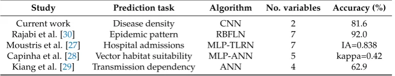
With respect to predicting epidemiological phenomena, a number of other studies have used artificial neural networks (ANN). For example, Moustris et al. [27] and Capinha et al. [28] applied Multi-layer Perceptrons (MLP) [26] to predict asthma admissions and habitat suitability for malaria vectors, respectively, using environmental and related variables. In an earlier study, Kiang et al. [29] used ANN to predict malaria transmission dependency on four environmental factors. The work most related to ours is that of Rajabi et al. [30] who used Radial Basis Functional Link Nets (RBFLN) [31] with environmental variables to predict Visceral Leishmaniasis distribution patterns. They posted 92 per cent accuracy, which is better than what is scored in the current study (81.6 per cent). This however, is expected given that the former study used a large number of risk variables (7) in their prediction model compared to what is used in the present study (2 risk variables for the case study disease [12]), see Table7.
Table 7.Classification accuracy (%) for ANN models on epidemic prediction tasks.
Study Prediction task Algorithm No. variables Accuracy (%)
Current work Disease density CNN 2 81.6
Rajabi et al. [30] Epidemic pattern RBFLN 7 92.0
Moustris et al. [27] Hospital admissions MLP-TLRN 7 IA=0.838 Capinha et al. [28] Vector habitat suitability MLP-ANN 5 kappa=0.42
Kiang et al. [29] Transmission dependency ANN 4 62.9
4. Materials and Methods
4.1. Data set
4.1.1. Population data
Figure 12.Population distribution data for year 2015 covering the study area.
4.1.2. Socio-economic data
The socio-economic data [33], a publicly available data set provides estimates of the proportion of poor people living in a 1kmx 1kmgrid in Uganda for the year 2015. Measurement of well-being is based on a multi-dimensional poverty index (MPI), which adopts a broad definition of well-being proposed by Alkire et al. [34]. The data in raster file format (geotiTIFF) was down-sampled from 1kmx 1kmto 250mx 250mgrid so as to be consistent with our spatial unit of analysis. The data was used as input for training our CNN models. The original data set was downloaded from the WorldPop website http://www.worldpop.org/.
4.1.3. Housing data
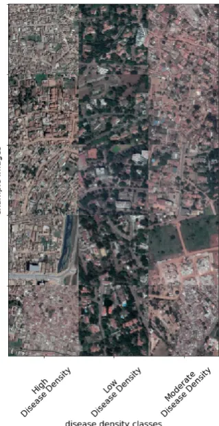
Figure 13.Example housing image data for study area extracted from Google Static maps API.
4.1.4. Epidemic data
The disease used as case study in this work isTuberculosis(TB), a high burden infectious disease and a leading cause of death among HIV/AIDS patients in Uganda [13] [14]. The data consists of monthly disease case counts for the year 2015 reported at sub-county level. It was acquired from the Health Management Information System version 2 (HMIS2), Ministry of Health, Uganda. The epidemic data was disaggregated from sub-county level counts to 250mx 250mgrid estimates using a method described in Section4.2.2.
4.2. Methods
4.2.1. Study area
The study area includes two large urban areas namely Kampala (the capital city) and Masaka in Uganda. Uganda lies between 10 29’ South and 40 12’ North latitude, 290 34 East and 350 0’ East longitude. These two urban centers are highly urbanized, have large populations, and report high infectious disease occurrence (especially TB and HIV/AIDS), which makes them suitable for the kind of analyses in this work. The spatial unit of analysis is a grid (cell) of size 250mx 250m(approx. 224 x 224 pixels), chosen to comply with satellite image extraction constraints and for easy analysis and interpretation of disease density prediction results.
4.2.2. Disaggregating and discretizing epidemic data
where a is fitting parameter, N is population size, and A is area size. We further tested this relationship by analyzing observational epidemic data with census population data at low spatial resolution and found significant positive correlation (p=0.000) and averager2=0.59. Before disaggregating the epidemic data to grid estimates, we first weighted each grid by its estimated population using Equation (2),
wi,j = ρi,j
∑sρ (2)
wherewis weight assigned to a grid located at the intersection of rowiand columnj, andρis its
population size. We now estimate disease countdat this grid using Equation (3) [37],
di,j=Ds∗w (3)
whereDsis disease count at the larger spatial unit (sub-county) in which grid at intersectioni,j
lies andwis the grid’s weight. Having disaggregated the epidemic data to grid scale, we needed to create disease density classes out of the data to make it a classification task. To do this we binned the normalized data such that each grid assumed a class depending on which bin its disease case estimate falls in. By following the procedure in [38] for binning population data, we created a matrixCwhere an entryCi,j= 0 if 0.66 <di,j=< 1.00, 2 if 0.33 <di,j=< 0.66, and 1 if 0.00 =<di,j=< 0.33 wheredi,jis normalized disease estimate. Table8provides details of disease density classes used in the present work. A summary of data sets used in this research is provided in Table9.
Table 8.Disease density classes used in the present work.
Value range Class Class label Sample count
0.67-1.00 0 High disease density 3,686 0.34-0.66 2 Moderate disease density 1,898 0.00-0.33 1 Low disease density 6,486
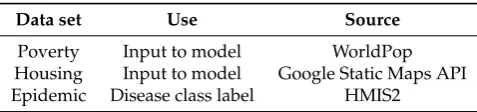
Table 9.Summary of data sets used in the present work.
Data set Use Source
Poverty Input to model WorldPop Housing Input to model Google Static Maps API Epidemic Disease class label HMIS2
All input data was pre-processed into appropriate feature vectors and normalized to (0, 1) value range by min-max scaling (Equation4) or, (1, 1) by standardizing (Equation5),
Xnorm= x−xmin
xmax−xmin (4)
z= x−µ
σ (5)
4.2.3. Model architecture and configuration
and/or socio-economic imagery data and outputs disease density class for a given geographical region of interest.
LetD be a grid of disease count values for a given geographical area at timet, C a grid of target disease class values,Ha grid of satellite images (depicting housing crowding), andEa grid of socio-economic indicator values. Thus, for every disease data valuedi,jand target class valueci,jthere is an associated satellite imagehi,jand socio-economic indicator valueei,j. We formulated the learning
task as estimating functiongusing Equation (6) for a multi-input, single-output prediction problem,
ci,j =g(hi,j,ei,j) (6)
where the multimodality (multi-input) representationci,jis computed using functiongbased on
unimodality (single-input) representationshi,j,ei,j (see [39] for a survey on multimodality machine learning). For CNN models based on overall unimodality architecture, representation learning was done using only one data source (either housing or socio-economic data) as shown in Equations7and 8, respectively.
ci,j=g(hi,j) (7)
ci,j=g(ei,j) (8)
In this work we used a CNN to estimate the functiongsince the mapping from input data to disease density estimate is non-linear, noisy, and dependent on semantic content of input data. An overview of the one-layer unimodality (single-input) and one-layer multimodality (multi-input) CNN network architectures are shown in Figures14and15, respectively.
Figure 14.Our one-layer unimodality CNN architecture for predicting disease density.
Figure 15.Our one-layer multimodality CNN architecture for predicting disease density.
Loss function Multi-class cross-entropy Learning rate 0.1 (halved every 10 epochs) Batch normalization (momentum = 0.9)
Weight initialization Random
Weight decay type (kernel regularizer) L2 (0.01)
Amount of weight decay 0.0002
Drop out Not used
Image data augmentation Yes
Bias initialization Zeros
Mini-batch size 32
Number of epochs 30
An architecture search space consisting of ten multimodality (Table10) and six unimodality architectures (Table11) for a total of sixteen, up to six layers deep, were evaluated. The goal was to identify a CNN architecture that was optimal for the nature and size of our data set.
Table 10.Architecture search space for multimodality CNN model (FE - feature extraction blocks).
Architecture FE before merging FE after merging Parameter count
One-layer 1 0 4,820,739
Two-layer A 1 1 679,875
Two-layer B 2 0 1,243,395
Three-layer A 2 1 151,395
Three-layer B 3 0 789,507
Four-layer A 2 2 132,387
Four-layer B 4 0 1,079,811
Five-layer 5 0 3,291,651
Six-layer A 3 3 357,411
Six-layer B 6 0 12,639,747
Table 11.Architecture search space for unimodality CNN model.
Architecture Feature Extraction blocks (FE) Parameter count
One-layer 1 2,410,371
Two-layer 2 641,091
Three-layer 3 226,563
Four-layer 4 150,723
Five-layer 5 159,555
Six-layer 6 188,931
Hyperparameter settings used for training our models are shown in Table12. The hyperparameter values were either obtained directly from the literature based on work using similar data set e.g., for learning rate and learning rate scheduling [21] or recommended best practices e.g., for weight initialization [40]. Settings specific to convolutional layers included a 3 x 3 (and 7 x 7) filter size, filter count of 64 (and 128), stride 1 x 1, and zero-padding as "same".
4.2.4. Model training
strategy allows for exploring of new network architectures that best fit the problem at hand in order to arrive at a robust model, which would not have been possible with transfer learning. Besides, there were no pre-trained multimodality CNN models in the public domain known to us by the time this study was conducted. Despite its advantages however, this strategy is laborious, time-consuming, and compute-intensive.
In developing and implementing each proposed CNN network architecture an iterative process was followed consisting of the following phases of activities: designing the architecture, training a model based on it, and analyzing/validating the model, Figure16. Once a satisfactory model was realized, it was trained on a combined data set of training and validation sets before evaluating on the test set. We applied the same regularization methods and other hyperparameter values to ensure uniformity across all architectures.
Figure 16. Overview of the iterative process we used to build a CNN model for predicting disease density.
4.2.5. Experimental setup
Training set 12,070 Test set 1,190
Total 13,260
4.2.6. Model evaluation
We used five standard evaluation metrics commonly used in machine learning research to evaluate the performance of our disease density prediction model. These include confusion matrix, overall accuracy, area under receiver operating characteristic curve (AUC/ROC), precision, recall, and F1-score. The decision to use multiple metrics is based on the reasoning that subjecting the resultant model to many different validation tests would give us a truly robust and highly generalizeable model. We employed visualization to gain further insight into and, explain model predictions using semantic features of input data i.e., housing and socio-economic image data. Our visualizations are based on a category of techniques called Class Activation Maps (CAM) which involve producing heatmap of class activations over input images. Unlike saliency maps [43] [44] that use gradients with output of the classification (dense) layer, the more general grad-CAM [17] [18] uses gradients with output of the last convolutional (or pooling) layer so as to utilize spatial information that gets completely lost in dense (classification) layers.
5. Conclusions
In this work we have considered the question of whether or not a CNN model can reasonably predict disease density from image-based urban housing and socio-economic data, especially in context of a developing country. Our experimental results show that CNN are promising for this task. In the current study, a CNN model built with a 1-layer depthwise separable convolution and appropriately optimized with a set of hyperparameters has the best predictive accuracy given our relatively small training data. Our model also generalizes fairly well to previously unseen data. Building signals extracted from satellite imagery was also found to be suitable input data source for predicting disease density using CNN. Despite the promising results achieved with a shallow architecture however, insufficient training data was found to be a limiting factor on the predictive performance of deeper and multi-input architectures. It would therefore, be interesting to know if and how predictive accuracy of multi-input architectures scales with larger training data. It is also worth noting that the current results were achieved with two risk variables for our case study disease. A multi-input CNN model for predicting disease density based on a larger number of risk variables would be an interesting research direction to pursue.
Author Contributions:Conceptualization, Rahman Sanya and Ernest Mwebaze; Data curation, Rahman Sanya; Investigation, Rahman Sanya; Methodology, Rahman Sanya; Resources, Rahman Sanya; Supervision, Gilbert Maiga; Validation, Rahman Sanya; Writing – original draft, Rahman Sanya; Writing – review & editing, Gilbert Maiga and Ernest Mwebaze.
Funding:This research received no external funding.
Conflicts of Interest:The authors declare no conflict of interest.
References
2. Ravi, D., Wong, C., Deligianni, F., Berthelot, M., Andreu- Perez, J., Lo, B., and Guang-Zhong. Deep learning for health informatics.IEEE Journal of Biomedical and Health Informatics2017, 21(1).
3. Marathe, M. and Vullikanti, A. K. S. Computational epidemiology.Communications of the ACM2013, 58(7), 88–96.
4. Garimella, V. R.K., Alfayad, A. and Weber, I. Social media image analysis for public health. CoRR2015, abs/1512.04476.
5. Ong, B. T., Sugiura, K., and Zettsu, K. Dynamically pre-trained deep recurrent neural networks using environmental monitoring data for predicting pm2.5.Neural Computing and Applications2016, 27, 1553–1566. 6. Dernoncourt, F., Lee, J. Y., Uzuner, Ö. and Szolovits, P. De-identification of patient notes with recurrent
neural networks.CoRR2016, abs/1606.03475.
7. Kendra, R. L., Karki, S., Eickholt, J. L. and Gandy, L. Characterizing the discussion of antibiotics in the twittersphere: What is the bigger picture?J Med Internet ResJun 2015, 17(6):e154.
8. Zou, B., Lampos, V., Gorton, R. and Cox, I. J. On infectious intestinal disease surveillance using social media content. InProceedings of the 6th International Conference on Digital Health Conference, DH ’16; ACM: New York, NY, USA, ACM, 2016; pp. 157–161.
9. Lecun, Y., Leon, B., Yoshua, B., Patrick, H. Gradient-based learning applied to document recognition. In Proceedings of the IEEE1998, 2278-2324.
10. Felbo, B., Sundsøy, P. R., Pentland, A., Lehmann, S. and de Montjoye, Y. Using deep learning to predict demographics from mobile phone metadata.CoRR2015, abs/1511.06660.
11. Phan, N., Dou, D., Piniewski, B. and Kil, D. Social restricted boltzmann machine: Human behavior prediction in health social networks. In2015 IEEE/ACM International Conference on Advances in Social Networks Analysis and Mining (ASONAM)Aug 2015, 424–431.
12. Kirenga, B. J., Ssengooba, W., Muwonge, C., Nakiyingi, L., Kyaligonza, S., Kasozi, S., Mugabe, F., Boeree, M., Joloba, M., Okwera, A. Tuberculosis risk factors among tuberculosis patients in Kampala, Uganda: Implications for tuberculosis control.BMC Public Health2015, 15(13), 1–7. doi:10.1186/s12889-015- 1376-3. 13. World Health Organization. Global tuberculosis report 2017. Technical report, 2017; World Health
Organization.
14. UNAIDS. Global report: UNAIDS report on the global aids epidemic.Technical report2013; United Nations. 15. Chollet, F. Xception: Deep learning with depthwise separable convolutions.CoRR2016, abs/1610.02357,
1610.02357.
16. Chollet, F. InDeep Learning with Python; Manning Publications Co: New York, U.S.A, 2018. 17. Kotikalapudi, R., contributors: keras-vis.GitHub2017.
18. Selvaraju, R.R., Abhishek, D., Ramakrishna, V., Michael, C., Devi, P., Dhruv, B. Grad-cam: Why did you say that? visual explanations from deep networks via gradient-based localization.CoRR2016, abs/1610.02391, 1610.02391.
19. Tobias, J. S., Alexey, D., Thomas, B., Martin, A. R. Striving for simplicity: The all convolutional net.CoRR 2014, abs/1412.6806, 1412.6806.
20. Sanya, R., Ernest, M. Mapping spatial housing patterns using Deep Neural Networks and remote sensing data. InNeural Information Processing Systems Conference 2018 Machine Learning for the Developing World,2018. 21. Albert, A.T., Kaur, J., Gonzalez, M.C. Using convolutional networks and satellite imagery to identify patterns
in urban environments at a large scale.ACM SigKDD 2017 Conference2017.
22. Cheng, G., Han, J., Lu, X. Remote sensing image scene classification: Benchmark and state-of-the-art. In Proceedings of the IEEE2017, 105(10), 1865–1883.
23. Jean, N., Burke, M., Xie, M., Davis, W. M., Lobell, D. B., Ermon, S. Combining satellite imagery and machine learning to predict poverty.Sciencemag2016, 353(6301), 790-794.
24. Basu, S., Ganguly, S., Mukhopadhyay, S., DiBiano, R., Karki, M., Nemani, R. DeepSat-A learning framework for satellite imagery.arXiv:1509.03602v1 [cs.CV] 11 Sep 2015.
25. Deng, J., Dong, W., Socher, R., Li, L.-J., Li, K., Fei-Fei, L. Imagenet: A large-scale hierarchical image database. IEEE Int. Conf. Comput. Vis. Pattern Recognit2009, 248–255.
mainland Portugal.Geospatial Health2009, 3, 177–187.
29. Kiang, R., Adimi, F., Soika, V., Nigro, J., Singhasivanon, P., Sirichaisinthop, J., Leemingsawat, S., Apiwathnasorn, C., Looareesuwan, S. Metereological, environmental remote sensing and neural network analysis of epidemiology of malaria transmission in Thailand.Geospatial Health2006, 1, 71–84.
30. Rajabi, M., Ali, M., Petter, P., Ahad, B. Environmental modelling of visceral leishmaniasis by susceptibility-mapping using neural networks: a case study in north-western Iran.Geospatial Health2014, 9(1), 179-191.
31. Looney, C. Radial basis functional link nets and fuzzy reasoning.Neurocomputing2002, 48, 489–509. 32. Facebook, L., Center for International Earth Science Information Network Columbia University. High
Resolution Settlement Layer (HRSL). Source imagery for HRSL 2016 DigitalGlobe.2016.
33. Tatem, A. J., Gething, P. W., Bhatt, S., Weiss, D., Pezzulo, C. Pilot high resolution poverty maps.2013. 34. Alkire, S., Santos, M. Acute multidimensional poverty: A new index for developing countries. Technical
report; UNDP-HDRO, New York, 2010.
35. Borremans, B., Jonas, R., Niel, H., and Herwig, L. The shape of the contact-density function matters when modelling parasite transmission in fluctuating populations. Royal Society Open Science 2017, 4, doi:10.1098/rsos.171308.
36. Hu, H., Karima, N., Philip, E. The scaling of contact rates with population density for the infectious disease models.Mathematical Biosciences2013, 244(2013), 125–134. doi:10.1016/j.mbs.2013.04.013
37. Sanya, R., Mwebaze, E. Using socio-economic well-being to predict geospatial epidemic intensity in a developing country setting. InAGILE 20182018.
38. Robinson, C., Fred, H., Bistra, D. A deep learning approach for population estimation from satellite imagery. CoRR2017, abs/1708.09086 1708.09086.
39. Baltrusaitis, T., Ahuja, C., Morency, L.-P. Multimodal Machine Learning: A Survey and Taxonomy. arXiv:1705.09406v2 [cs.LG]2017.
40. Patterson, J. and Adam, G. InDeep Learning: A Practitioner’s Approach; Loukides, M., McGovern, T., Eds.; O’Reilly Media Inc: Sebastopol, U.S.A, 2017.
41. Chollet, F., et al. Keras.GitHub2015.
42. Abadi, M., Agarwal, A., Barham, P., Brevdo, E., Chen, Z., Citro, C., Corrado, G., Davis, A., Dean, J., Devin, M., Ghemawat, S., Goodfellow, I., Harp, A., Irving, G., Isard, M., Jia, Y., Kaiser, L., Kudlur, M., Levenberg, J., Man, D., Monga, R., Moore, S., Murray, D., Shlens, J., Steiner, B., Sutskever, I., Tucker, P., Vanhoucke, V., Vasudevan, V., Vinyals, O., Warden, P., Wicke, M., Yu, Y., Zheng, X. TensorFlow: Large-scale machine learning on heterogeneous distributed systems.arXiv preprint2015, 1603.04467.
43. Smilkov, D., Nikhil, T., Been, K., Fernanda, B.V., Martin, W. Smoothgrad: removing noise by adding noise. CoRR2017, abs/1706.03825. 1706.03825.
44. Karen, S., Andrea, V., Andrew, Z. Deep inside convolutional networks: Visualising image classification models and saliency maps.CoRR2013, abs/1312.6034, 1312.6034.