SEGMENTATION AND ANALYSIS METHOD FOR TWO-PHASE CERAMIC (HfB2-B4C) BASED ON THE DETECTION OF VIRTUAL BOUNDARIES

SEGMENTATION AND ANALYSIS METHOD FOR TWO-PHASE CERAMIC

(HFB

-B

C) BASED ON THE DETECTION OF VIRTUAL BOUNDARIES

Y

H

C

L

B

W

T

H

D

H

H

G

1_{School of Computer Engineering and Science, Shanghai University, 99 Shangda Road, Shanghai, China;} 2_{Shanghai Institute for Advanced Communication and Data Science, Shanghai University, Shanghai, China;} 3_{School of Materials Science and Engineering, Shanghai University, 99 Shangda Road, Shanghai, China;} 4_{Material Genome Institute, Shanghai University, 99 Shangda Road, Shanghai, China}

e-mail: [email protected], [email protected], [email protected], [email protected], dlhu [email protected], [email protected]

(Received July 30, 2018; revised October 23, 2018; accepted December 8, 2018)

ABSTRACT

Microstructure of a material stores the genesis of the material and shows various properties of the material. To efficiently analyse the microstructure of a material, the segmentation of different phases or constituents is an important step. However, in general, due to the microstructure’s complexity, most of segmentation is manually done by human experts. It is challenging to automatically segment the material phases and the microstructure. In this work, we propose a method which combines the the dilation operator, GLCM (gray-level co-occurrence matrix), Hough transform and DBSCAN (density-based spatial clustering of applications with noise) for phases segmentation in the examples of certain material of eutectic HfB2-B4C ceramics. In the segmented regions, the further analysis for the microstructural elements is done with DBSCAN. The experimental results show that the proposed method achieves 95.75% segmentation accuracy for segmenting phases and 86.64% correct classification rate for the microstructure in the segmented phases. These experimental results show that our method is effective for the difficult task of the both segmentation and classification of the microstructural characteristics.

Keywords: boundary detection, clustering algorithm, image segmentation, two-phase microstructure, virtual boundary.

INTRODUCTION

In the research field of ceramic materials, the imaging and analysis of ceramic microstructure are important base for studies of the structure-property relationship. By understanding the characteristics of different microstructures, it is possible to establish the quantitative correlation between the microstructure behaviours and desired properties. Such correlations could be beneficial for the development of ceramic materials (Chermant, 1986; Vales et al., 1999). However, traditional analysis of the ceramic microstructures is mainly performed manually with low efficiency and only for primitive characteristics. Therefore, applying the computer image processing technology to analyse the ceramic microstructure more accurately and in more elaborate way has become a research focus in recent years (Yang et al., 2009a;b; Toddet al., 2016).

The eutectic HfB2-B4C ceramics (made from

electric charge melting technique) consist of two phases inter-twinned with each other, hence to form a special two-phase microstructure at the mesoscopic scale. The eutectic relationship between HfB2 and

B4C phases is ideally fixed. However, the phase

ratio may change from one region to another within the two-phase microstructure. In another word, the eutective relation could vary at the mesoscopic level, hence it is necessary to identify and recognize such variations. Two images of such two-phase microstructure from HfB2-B4C ceramics are shown

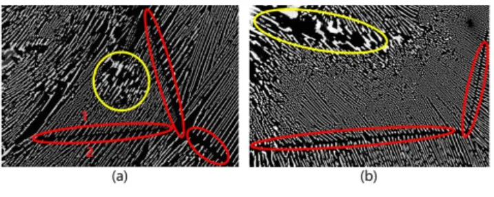
in Fig. 1. In these microstructures, the regions with white elements are clearly separated by the black straight gaps which are marked in red ellipses, hence defining different microstructural regions. These regions are relatively independent, especially the white elements distributed regularly with distinctive behaviour in each region. The relationship between the microstructures and properties of eutectic HfB2-B4C

Fig. 1. (a) and (b) are two images about HfB₂-B4C

ceramics. In the two images, the white microstructural elements are divided by the black straight gaps which are marked in red ellipses, and form the discrete regions. The microstructural elements in the yellow circle are different from the other microstructural elements in the same region, and form the independent subregion.

There have been several methods related to the segmentation of the ceramic microstructure. Cai et al. (2013) proposed a segmentation method based on mean shift. The method can give the satisfactory results on alumina ceramic images and ceramic tile images. Ananyev et al. (2014) and Lopez et al. (2015) both applied the morphological filter in the segmentation and quantification of microstructures in the ceramic images. Haha et al. (2007) segmented the SEM (scanning electron microscopy) images of motar with a threshold segmentation method, extracted the microstructures under different grayscale range. Zhao et al. (2016) conducted the segmentation of the ceramic BSE (backscattered electron) images by spectral clustering algorithm. The experiment results showed that their algorithm is appropriate for some ceramic images which have complex texture. Chen et al. (2014) improved the traditional watershed method to solve the over-segmentation problem in the segmentation of the images.

However, all the images processed in the above mentioned researches have real boundaries or high contrast among different regions. The real boundaries refer to the real dividing curves or areas with strong contrast, such as the boundaries between white microstructural elements and black region in Fig. 1. When dealing with ceramic images which only have straight gaps among different regions as illustrated in Fig. 1, it’s hard to directly detect the boundaries among regions and accurately segment the regions with the above mentioned methods. The straight gap is called “virtual boundary” (VB) here. The VB is similar to the reification of illusory contour in the gestalt psychology (Leharet al., 2003). The VB can be easily perceived by human visual system, but it is difficultly detected for computers.

There were several research works to segment the materials images without obvious boundaries.

Vanderesse et al. (2008) presented an algorithm of 3D titanium alloy image segmentation based on the orientation of the lamellae. Jeulin et al. (2008) introduced a local orientation estimator to locate fast changes of textures orientation, and to make a segmentation based on different orientations. The Both works made use of the microstructural orientation feature, and obtained good segmentation results on 2D and 3D materials images. The premise of the two works is that the microstructures in similar orientations belong to the same region, and the microstructures in different orientations belong to different regions. However, this premise is not suitable for the images of HfB2-B4C ceramics. As shown in Fig. 1 (a), although

the microstructures in region 1 and the microstructures in region 2 have similar orientations, they are still two regions because they are separated by a straight gap, i.e., a VB.

In general, the detection of the VBs is the key to segment discrete regions in the images of HfB2

-B4C ceramics. However, most of the existing boundary

detection methods (Osheret al., 2006; Liet al., 2011; Muthukrishnan et al., 2011) are designed for the real boundaries. In addition, there are also different types of microstructural elements in each region, and form the independent subregions as marked in yellow ellipses in Fig. 1. To perform the quantitative analysis of the ceramic microstructure, the different microstructural elements in each region also need to be identified and segmented. Therefore, in this paper, we focus on the accurate detection for the VBs in the images of HfB2-B4C ceramics and the classification for the

microstructural elements in each discrete region.

In order to detect the VBs, we propose a method based on the dilation operator and the GLCM (gray-level co-occurrence matrix) to eliminate the gaps among microstructural elements and retain gaps among discrete regions. Then, the Hough transform method is used to detect straight lines based on the retained gaps. After these detected straight lines are further processed, the final VBs are obtained, and the discrete regions are segmented with the VBs. Finally, for each region, the microstructural elements are classified through the DBSCAN (density-based spatial clustering of applications with noise) method. The experimental results show that our approach has high segmentation precision, and is able to classify different microstructural elements effectively.

reported and discussed. Finally, a conclusion is drawn in Section “Conclusion”.

THE PROPOSED APPROACH

The proposed method consists of two parts: one is the segmentation of the discrete regions; the other one is the classification for the microstructural elements in each discrete region. Since the discrete regions are mainly separated through the VBs, the VBs need to be firstly detected as the main task in the first part. In the second part, microstructural elements in each segmented region are classified into different classes to analyse the transformation of the microstructural elements.

THE SEGMENTATION OF THE DISCRETE REGIONS

The key in the segmentation of the discrete regions is to detect the VBs. In order to obtain the VBs, four steps are utilized: pre-processing, filling the gaps among microstructural elements, detecting the candidate boundary lines, filtering and processing the candidate boundary lines.

Pre-processing for the ceramic image

With the SEM(scanning electron microscopy), we can obtain high-resolution images for microstructure objects. Most of the ceramic microstructure images have very large sizes, such as 4096×3072 pixels. Although the high resolution image can provide more details for the observed objects, the large size reduces the efficiency of the following image processing and analysis steps. Since the VBs are obvious, they can quickly detected after reducing the large images. Therefore, to speed up the next processing steps, the ceramic microstructure images are scaled firstly. Here, the width of the images are scaled to 512 pixels and the height of the images are also scaled to keep the aspect ratio. Furthermore, resizing the original images can facilitate the selection of parameters which are used in the following steps.

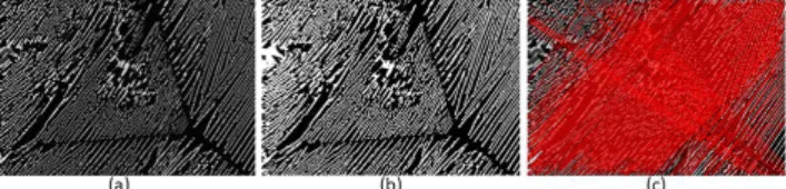
As shown in Fig. 2(a), the microstructural elements are gray, and the background is black. To enhance the contrast between the microstructural elements and background, the images need to be binarized with the Otsu method (Otsu, 1979), as illustrated in Fig. 2(b). After the binarization, all the microstructural elements turn to pure white, and the background turns to pure black. Thus, the extraction of the microstructural elements becomes much easier, and this also increases the efficiency of the following steps.

Fig. 2. (a) The original image; (b) the result of the binarization; (c) the detected lines with the Hough transform method.

Filling the gaps among microstructural elements

In fact, the VBs are the curves of illusion, which can be observed by humans. However, they are difficultly perceived by the computer. The virtual boundary’s areas are the gaps among the discrete regions, as marked by red ellipses in Fig. 1. In general, these gaps are some line segments which have a certain width. Thus, the detection of the VBs can be converted to detecting the straight lines. However, the gaps among microstructural elements hinder the detection of the VBs, e.g., creating many wrong lines with the Hough transform method (Hough, 1962), as shown in Fig. 2(c) which is the result of lines detection from the Fig. 2(b). Therefore, the primary task is filling the gaps among microstructural elements and retaining the gaps among discrete regions. To achieve this purpose, two methods are adopted here.

First, the dilation operation (Serraet al., 2012) is applied. Since most of the gaps among microstructural elements are more narrower than the ones among discrete regions, the thin gaps are filled and the VBs are left with the dilation operation. If the values of a pixel (x0,y0) and its neighbour pixels (xi,yj) are defined asI(x₀,y₀)andI(xi,yj), respectively, then the relation of the dilated valueI0(x0,y0)with a square of

sizel1as structuring element andI(xi,yj)is shown as following:

I0(x0,y0) =max

I(xi,yj)|x0−

l1

2 6xi6x0+ l1

2,

y0−

l1

2 6yj6y0+ l1

2

.

(1)

Through the dilation operation, the value of pixel (x0,y0) is replaced by the maximum in its

neighbourhood. The larger the l1 is, the more the

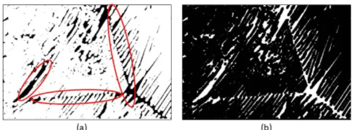
Fig. 3. (a) is the dilation result of Fig. 2(b), and the remained gaps are marked in red ellipses. (b) is the inverse binarization of (a) to highlight the remained gaps.

The second method is based on the gray-level co-occurrence matrix (GLCM; Haralick et al., 1973). If the microstructural elements are regarded as textures, then for the gaps among discrete regions, most of the local area is black, i.e., the textures change little; for the gaps among microstructural elements, the local area is chequered with black and white, i.e., the textures change a lot. With the theory of GLCM, the variance of contrasts in different directions are able to reflect the distributions of the textures. In other words, the larger the variance in the GLCM is, the greater the degree of textures change (Xian, 2010). With the GLCM, all variance of contrast in local area can be calculated. Then, the areas with small variance are considered as the gaps which need to be preserved. To be specific, an image is firstly divided into small squares with a side length of l2. For each l2∗l2

square f, the GLCMGε α is calculated. ε andα are

the distance and orientation between the pixel pairs, respectively. Ifg_(m,n)is defined as the value of them -th row and -then-th column in a matrixGε α, theng(m,n) is calculated by the following equation:

g_(m,n)=#

(x1,y1),(x2,y2)∈l2∗l2| f(x1,y1)=m,

f_(x2,y₂)=n, q

(x2−x1)2+ (y2−y1)2=ε,

arctan

y2−y1

x2−x1

=α

,

(2) where #{∗}is the total number of elements in set{∗}; f_(x,y) is the grayscale value of the pixel (x,y) in the square f;(x₁,y₁)is the reference pixel; (x₂,y₂)is the pixel which at a distance ofεfrom the reference pixel

(x₁,y₁) in the directionα. In our method, theε is set

to 2, and choose four direction (0◦,45◦,90◦,135◦)to calculate four GLCMs{G_{2 0}◦,G_{2 45}◦,G_{2 90}◦,G_{2 135}◦}

for a square. According to Eq. 2, matrixGε α isNg∗Ng whereNgis the gray levels and it is set to 8 here. Matrix

Gε α records the times of various pixel pairs appears.

To reflect the textures characteristics, the probability of

various pixel pairs appears is needed. Hence, theGε α

needs to be further calculated as following:

p_(m,n)= g(m,n)

∑ N_g i,j=1g(i,j)

, (3)

where p_(m,n) is the value of the m-th row and the n-th column in a matrix Pε α, which records the

probability of various pixel pairs appears; g_(m,n) and g_(i,j) are elements in the matrix G_{ε α}. Then, the contrast CONε α can be computed throughPε α:

CONε α=

N_g

∑

p_(m,n)(m−n)2, (4)

wherep_(m,n)is the element in the matrixP_{ε α}.

As mentioned above, four GLCMs are calculated in four direction for a square. Therefore, four matrixs (P2 0◦,P2 45◦,P2 90◦,P2 135◦) and four contrasts

(CON2 0◦, CON2 45◦, CON2 90◦, CON2 135◦) can be

obtained for a square. The four contrasts describe the degree of color difference in four directions. If the four contrasts are very different, the textures in the square are messy. To make use of this characteristic in the four contrasts, the variance of the four contrasts is calculated, denoted asVAR. The larger theVARis, the messier the textures are. The Fig. 4(a) visualizes the variance of each square, the variance of each square is scaled to[0,255]. Then, the squares with the smallest variance 0 are remained. Specifically, if the VAR of a square is less than 1, the square is remained in white; otherwise, the square is discarded in black. This process is equivalent to the inverse binarization of Fig. 4(a) with threshold 1. The remained squares are displayed in Fig. 4(b) and the VBs are on the remained squares.

Fig. 4. The results with the GLCM method. (a) The visualization for the variance of each square. (b) The inverse binarization image from (a).

Detection of candidate boundary lines

For each pixel p which belongs to the remained gaps and the coordinate of p is (x,y), the family of straight lines which go through this pixelpis defined as:

r=xcosθ+ysinθ (0≤r,0≤θ≤2π), (5)

whereris the distance from the origin of coordinates to the straight line;θ is the angle between thex axis

and the perpendicular of the straight line. The family of straight lines can be represented by a group of pairs

(r,θ), and form a curve in ther-θplane. Therefore, the

collinear pixels are corresponding to a family of curves which intersects at the same point in ther-θplane. The

more curves that intersects at a same point, the more pixels are in the same straight line which corresponds to the intersection point. Thus, the detection of the straight lines in a image can be achieved by checking the intersection points of curves inr-θplane.

The Hough transform method is conducted respectively on the two kinds of remained gaps which are obtained by the above mentioned two methods (the dilation method and the GLCM method), as illustrated in Fig. 5(a) and Fig. 5(b). If lines detection is performed only on the remained gaps obtained by the dilation method or the GLCM method, then the number of lines detected on some thin gaps tends to be small. These lines are likely to be removed as noise due to insufficient quantity in the following filtering step. Simply copying the detected lines and increasing the number of them by several times can also increase the noise several times. Therefore, the both methods are needed. The detected lines based on the two methods are combined to ensure that the lines on the thin gaps are sufficient without increasing the noise. The combined result is shown in Fig. 5(c). It still contains some redundant boundary lines and erroneous boundary lines. These detected straight lines can only be regarded as candidate boundary lines and need further to be processed.

Fig. 5. The results of the Hough transform method. (a) The lines are detected with the Hough transform method based on the dilation method. (b) The lines are detected with the Hough transform method based on the GLCM method. (c) The red lines are obtained by combining the detected lines in (a) and (b).

Filtering and processing of the candidate boundary lines

There are mainly two issues need to be dealt with in the candidate boundary lines. The first issue is filtering the redundant line segments which are in the same boundary region and eliminating the wrong line segments; the second issue is extending the retained line segments to form a whole boundary of the discrete regions.

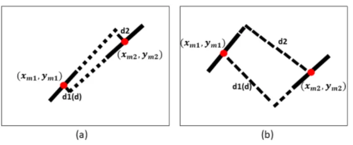
To solve the first issue, the candidate boundary lines are grouped by the distance and the slope firstly. In our approach, the distance d between two line segments is calculated as follows:

d=min

A1xm2+B1ym2+C1 q

A2₁+B2₁

,

A₂xm1+B2ym1+C2 q

A2₂+B2₂

!

, (6)

where(A1,B1,C1)and(A2,B2,C2)are the coefficients

of equations of two line segments, respectively;

(xm1,ym1)and(xm2,ym2) are the midpoints of the two

line segments, respectively. As shown in Fig. 6, if the distance d between the two line segments is less than a threshold 10 and the angle between the two line segments is smaller than 10◦, then the two line segments are divided into the same group. In the process of grouping, for each line segment, the number of microstructural elements which are gone through by the line segment is also computed, and denoted asη.

To eliminate the influence of the different lengths of line segments, theηis need to be divided by the length

of line segmentlen, and the result is denoted asγ,i.e., γ=η/len. If theγof a line segment exceeds threshold σ, the line segment is discarded and not be grouped.

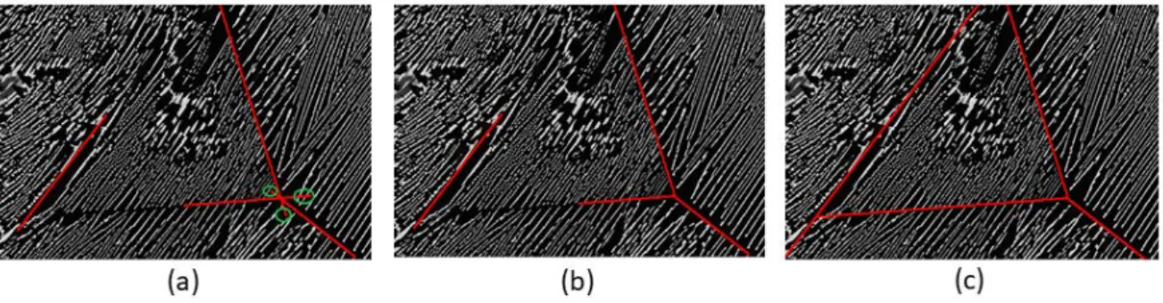
Fig. 7.The results of boundaries processing. (a) The result of boundaries filtering: the red line segments marked by green circles are the redundant threads. (b) The result of threads removing: the redundant threads in image (a) are removed. (c) The result of lines extension: the line segments in (b) are extended to form the final VBs.

Then, for each group, selecting one line segment whose γ is the minimum as the final line segment in

this group. The filtering result of candidate boundary lines is shown in Fig. 7(a).

Furthermore, the remained line segments still need to be extended to form the intact boundaries. As demonstrated in Fig. 7(a), some remained line segments intersect and generate the redundant threads marked in green circles. These threads need to be removed before extending the line segments. Specifically, the line segments are measured from the intersection to the end points. Then, the removing of the threads can be achieved by remaining the longest section and removing other sections, the result is shown in Fig. 7(b). At this point, the line segments are extended if they are not closed. The line segments are extended from its two ends until reaching the boundaries of whole image or intersecting the other lines. The final VBs are shown in Fig. 7(c).

THE FURTHER ANALYSIS AND CLASSIFICATION FOR THE

MICROSTRUCTURAL ELEMENTS

Feature extraction for microstructural elements

Although the discrete regions can be segmented by the VBs, there are some microstructural elements with different characteristics in the same discrete region, such as the microstructural elements in red ellipses in Fig. 8(a) and (b). To analyse the transformation of the microstructural elements in the same discrete region, it’s necessary to distinguish microstructural elements with different characteristics and further partition the

Fig. 8.The different microstructural elements. (a) The microstructural elements have different widths in a discrete region. (b) The microstructural elements have different orientations in a discrete region.

discrete regions. In this paper, the classification of the microstructural elements involves feature extraction and machine learning. For the images of HfB2-B4C

the major differences between these microstructural elements are the direction and size. Thus, two features are extracted for each microstructural element.

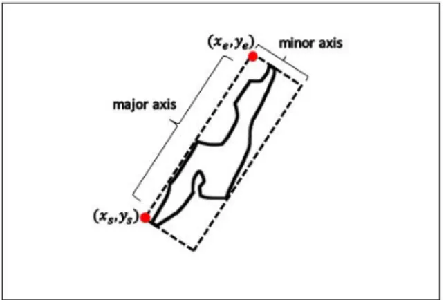
The first feature is major slope (Fm). Fm describes the orientation of the major axis of each microstructural element. An example is shown in Fig. 9. the minimum oriented bounding box of a microstructural element is calculated. The long side of the rectangle is regarded as the major axis. The slope of the major axis is computed as the major slopeFm:

Fm=ye−ys xe−xs

, (7)

Fig. 9. The minimum oriented bounding box of a microstructural element.

The second feature is width (Fw) which is the length of the minor axis of each microstructural element. The minor axis refers to the short side of the oriented bounding box, as demonstrated in Fig. 9. Since the main difference in the shape of microstructural elements is the length of the minor axis, such as the different elements in Fig. 8(a), Fw is competent for the distinguishing of different shapes.

Through feature extraction, a two dimensional feature vector Fi can be obtained for i-th microstructural element, composed as the two essential cues:

Fi= [Fim,F w

i ]. (8)

In addition, since the scales of the two features are different, the two features need to be normalized to

[0,1]respectively before they are used to classify the microstructural elements.

Classification for the microstructural elements

For the normalized feature vectors, due to the lack of the labels, an unsupervised machine learning method which is density-based spatial clustering of applications with noise (DBSCAN; Esteret al., 1996) is adopted here.

DBSCAN is a density-based clustering algorithm without specifying the number of clusters. Given a set of data in feature space, high-density regions can be discriminated from low-density regions. In addition, DBSCAN can be used for arbitrarily shaped clusters and it is robust to noises. The DBSCAN needs two parameters: the minimum number of points minPts required in the neighbourhood of a core point and the neighbourhood sizeEps. The two parameters minPts andEpscan affect the result of clustering. If theEpsis too small or theminPtsis too large, the number of core points is small, and the data is easy to be over-classified or mistaken for the noises. If the Eps is too large or

the minPtsis too small, the number of core points is large, and the data is easy to be under-classified or some noises can not be detected.

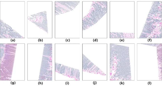
With the DBSCAN, the microstructural elements can be classified. To illustrate the classification result, the microstructural elements which are in different classes are painted with different colors, as shown in Fig. 11. The classification result can illustrate well the characteristics of the distribution and transformation of the microstructural elements.

PARAMETER SELECTION

In the proposed approach, three parameters

[l₁,l₂,σ] in Section “Filling the gaps among

microstructural elements” are keys for the segmentation of the discrete regions. In general, for the images with wide gaps among discrete regions, it tends to choose large values of[l1,l2]and a small value

ofσ; and for the images with thin gaps among discrete

regions, it tends to choose small values of [l1,l2]and

a large value of σ. Through the experiments, good

detection results can be achieved when the value ofl2

is set tobl1/2c. Hence, only thel1needs to be set. And

the range ofl₁is{3,5,7,9}, the range ofσis[0.1,0.5].

In the second part of our approach, the parameters Eps and minPts in DBSCAN are also need to be considered. Generally, for each discrete region, if there are significant differences among microstructural elements in the region, then smallEpsand largeminPts are used; otherwise, large Eps and small minPts are applied. The range ofEpsis[0.01,0.05], and the range ofminPtsis[5,30].

EXPERIMENTAL RESULTS AND

DISCUSSIONS

In order to evaluate the performance of our method, the proposed method is tested on ten images of the HfB2-B4C ceramics which are shown in

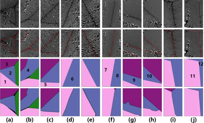
Fig. 10. As introduced above, the proposed method mainly includes two parts: segmentation of the discrete regions; further analysis and classification for microstructural elements. For the tested images, the results of segmentation is shown in Fig. 10. Twelve segmented regions are chosen to validate the further analysis and classification method, the results is illustrated in Fig. 11. The segmentation of the discrete regions is composed of pre-processing, filling of the gaps, lines detection and lines filtering, and there are two parameters [l1,σ] need to be set. The

setting of parameters [l1,σ] for the ten images are

[3, 0.2], [5, 0.2], [7, 0.1] and [5, 0.2], respectively. For the DBSCAN in the second part, the parameters

[Eps,minPts]for the twelve regions are set as follow: [0.05,20], [0.02,20], [0.05,15], [0.02,15], [0.03,20], [0.05,25], [0.03,20], [0.05,20], [0.05,20], [0.05,20], [0.02,20] and [0.03,10].

In Fig. 10, the VBs of the ten ceramic’s microstructural elements are detected, and the discrete regions are segmented through the boundaries. To verify the effect of the segmentation, an evaluation criterion which is called segmentation accuracy is utilized. The segmentation accuracy SegAcc is computed by the following equations:

SegAcc=AC AS

, (9)

AC=

∑

AMi∩ADi, (10)

whereAMi is the area of ith region marked manually;

ADiis the area ofith region segmented by our method;

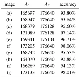
AC is the area of regions segmented correctly; AS is the total area of the image. AC can be obtained by computing the number of pixels which have the same color between segmentation results and ground truth as shown in Fig. 10. The segmentation accuracy SegAcc reflects the proportion of the correct part in segmentation result. Table 1 shows the segmentation accuracy of the ten images in Fig. 10:

In Table 1, “(a)” to “(j)” in the column “image” represent the original images of column (a) to (j) in Fig. 10. From table 1, the segmentation accuracy of the ten images in Fig. 10 are all more than 90%, and the average segmentation accuracy is 95.75%. Through the column (a), (h) and (i) in Fig. 10, which have

Table 1.The segmentation accuracy of our method

image AC AS accuracy

(a) 165697 176640 93.80% (b) 168947 176640 95.64% (c) 168379 176128 95.60% (d) 171089 176128 97.14% (e) 169341 175104 96.71% (f) 173205 176640 98.06% (g) 168742 176640 95.53% (h) 164070 176640 92.88% (i) 166269 176640 94.13% (j) 173133 176640 98.01%

the lower segmentation accuracy, there are two main sources of error: first, the gaps among regions are too wide to pinpoint the position of the boundary lines, such as the gap between pink region and blue region in image of column (a), row 4 in Fig. 10; second, the gap is not similar to a straight line, such as the gap between pink region and blue region in image of column (h), row 4 in Fig. 10, and the gap between purple region and blue region in image of column (i), row 4 in Fig. 10. Another important factor that causes errors is the gaps are too thin to detect the boundary lines, such as the gaps around the small purple region in image of column (f), row 4 in Fig. 10, and the gap between purple region and blue region in image of column (g), row 4 in Fig. 10. The detection of the boundary lines in the wide and linear gaps is able to achieve high accuracy, such as the column (c), (d), (e) and (j).

The Fig. 11 shows the classification results of the microstructural elements in twelve discrete regions, which are corresponding to the regions 1 to 12 of row 3 in Fig. 10. To evaluate the accuracy of our method in the classification of the microstructural elements, the correct classification rate (CCR) (Diplaroset al., 2007) is calculated as the evaluation criterion. The CCR is defined as:

CCR=

N

∑

|hkTck|

H , (11)

H=

N

∑

hk, (12)

wherekis thek-th class;Nis the number of the classes; hk is the number of the microstructural elements in

k-th class with our method; ck is the actual number of the microstructural elements in k-th class which are counted by human. By the definition of CCR, the higher the CCR, the higher the accuracy of the classification. The CCR of the classification of the microstructural elements in the twelve regions are shown in Table 2:

Table 2. CCR of the classification for the micro-structural elements

region CCR region CCR region CCR

(a) 0.8234 (e) 0.8389 (i) 0.8922

(b) 0.8526 (f) 0.9070 (j) 0.8625

(c) 0.9032 (g) 0.8615 (k) 0.8701

Fig. 10.The segmentation of the discrete regions. Row one is ten original ceramics images. Row two is the results of boundaries detection. Row three is the segmentation results based on the detected boundaries. Row four is the ground truth marked by human. The regions 1-12 of row 3 are chosen to validate the further analysis and classification method.

In Table 2, “(a)” to “(l)” in the column “region” represent the images (a) to (l) in Fig. 11, respectively. TheCCRof the twelve regions are all more than 0.8, and the averageCCRis 0.8664. For each region, if the microstructural elements have significant differences in shape, the CCR of the region is high, such as the values of regions “(c)”, “(f)”, “(h)”, “(i)” and “(k)” in Table 2. On the other hand, if most of the microstructural elements in the region are similar, the CCRof the region is low, such as the regions “(a)” and “(e)”.

CONCLUSION

In this work, a method using the dilation operator, GLCM, Hough transform and DBSCAN is proposed to accurately segment the images of HfB2-B4C

ceramics with many VBs and further classify the different microstructural elements in each segmented region. The experiments demonstrate that the proposed method can effectively detect the VBs and further obtain the accurate segmentation. In addition, the two features “Major Slope” and “Width” which are extracted for the microstructural elements are proved to be effective in the classification. The classification based on the DBSCAN is also able to be achieved

precisely. Thus, the proposed method provide a reliable technical support to effectively analyse the HfB2-B4C ceramics microstructure.

We conclude that our method is an effective and robust way to segment the material regions with VBs. However, there are two limitations which need to be improved. On the one hand, the method is difficult to detect non-linear VBs since it is based on the Hough transform method; on the other hand, the detection of the VBs in some thin gaps is failed with our method. We will continue to research to overcome the shortcomings in the future work.

ACKNOWLEDGMENTS

Fig. 11. The classification of microstructural elements in each discrete region. (a) to (l) are twelve regions corresponding to the regions 1 to 12 of row 3 in Fig. 10. In each image, the microstructural elements which have the same color belong to the same class.

REFERENCES

Ananyev M, Medvedev D, Gavrilyuk A, Mitri S, Demin A, Malkov V, Tsiakaras P (2014). Cu and Gd co-doped BaCeO 3 proton conductors: Experimental vs SEM image algorithmic-segmentation results. Electrochim Acta 125:371–9.

Chermant JL (1986). Characterization of the microstructure of ceramics by image analysis. Ceram Int 12(2):67–80. Cai HH, Cheng Y, Liu BX (2013). Ceramic microstructure image segmentation by mean shift. Appl Mech Mater 423:2602–5.

Chen Y, Chen J (2014). A watershed segmentation algorithm based on ridge detection and rapid region merging. In: Proc 2014 IEEE Int Conf Signal Process Commun Comput (ICSPCC), 420–4.

Diplaros A, Vlassis N, Gevers T (2007). A spatially constrained generative model and an EM algorithm for image segmentation. IEEE T Neural Networ 18(3):798– 808.

Ester M, Kriegel HP, Sander J, Xu X (1996). A based algorithm for discovering clusters a density-based algorithm for discovering clusters in large spatial databases with noise. In: Proc 2nd Int Conf Knowledge Discover Data Mining (KDD-96), 226–31.

Haralick RM, Shanmugam K (1973). Textural features for image classification. IEEE T Syst Man Cyb 6:610–21. Haha MB, Gallucci E, Guidoum A, Scrivener KL (2007).

Relation of expansion due to alkali silica reaction to the degree of reaction measured by SEM image analysis.

Cement Concrete Res 37(8):1206–14.

Hough PV (1962). Method and means for recognizing complex patterns. U.S. Patent 3,069,654.

Jeulin D, Maxime M (2008). Segmentation of 2D and 3D textures from estimates of the local orientation. Image Anal Stereol 27(3):183–92.

Lehar SM (2003). The world in your head: A gestalt view of the mechanism of conscious experience. Mahwah: Lawrence Erlbaum Assoc, pp 91–105.

Li H, Liao X, Li C, Huang H, Li C (2011). Edge detection of noisy images based on cellular neural networks. Commun Nonlinear Sci 16(9):3746–59.

Lopez P, Lira J, Hein I (2015). Discrimination of Ceramic Types Using Digital Image Processing by Means of Morphological Filters. Archaeometry 57(1):146–62. Muthukrishnan R, Radha M (2011). Edge detection

techniques for image segmentation. Int J Comput Sci Inform Tech 3(6):259–67.

Otsu N (1979). A threshold selection method from gray-level histograms. IEEE T Syst Man Cyb 9(1):62–6. Osher S, Fedkiw R (2006). Level set methods and dynamic

implicit surfaces. New York: Springer.

Serra J, Soille P, eds. (2012). Mathematical morphology and its applications to image processing. Dordrecht: Springer.

Vanderesse N, Maire E, Darrieulat M, Montheillet F, Moreaud M, Jeulin D (2008). Three-dimensional microtomographic study of Widmansttten microstructures in an alpha/beta titanium alloy. Scripta Mater 58(6):512–5.

Vales F, Rezakhanlou R, Olagnon C (1999). Determination of the fracture mechanical parameters of porous ceramics from microstructure parameters measured by quantitative image analysis. J Mater Sci 34(16):4081–8. Xian GM (2010). An identification method of malignant and benign liver tumors from ultrasonography based on GLCM texture features and fuzzy SVM. Expert Syst

Appl 37(10):6737–41.

Yang Y, Guo Y (2009). Application of digital image technology to ceramic micro-image processing. Comput Eng Design 30(3):1008–9.

Yang Y, Guo Y, Wang X (2009). Digital image technology assistant for the quantitative analysis of the ceramics microstructure. Mater Rev 23(14):83–6.