Sensory Input Transformation in Layer 4 of Primary Somatosensory Cortex
Peng Gong
A dissertation submitted to the faculty of the University of North Carolina at Chapel Hill in partial fulfillment of the requirements for the degree of Doctor of Philosophy in
the Department of Biomedical Engineering.
Chapel Hill 2008
Approved by,
Advisor: Associate Professor Oleg V. Favorov
Reader: Professor Henry S. Hsiao
Reader: Professor Douglas G. Kelly
Reader: Associate Professor Mark Tommerdahl
iii
ABSTRACT
Peng Gong: Sensory Input Transformation in Layer 4 of Primary Somatosensory Cortex
(Under the direction of Dr. Oleg V. Favorov)
Neural representation of sensory information in the cerebral cortex undergoes
a series of transformations, starting from its initial form at the level of thalamic
neurons through a succession of cortical layers of multiple cortical areas. In the
somatosensory system, the first such transformation takes place in the input layer, or
Layer 4, of area 3b. This study explores several of its known properties: (1) the
cortex is organized as a set of minicolumns, each a radial cord of cells 30-50 μm in
diameter; (2) receptive fields of neighboring minicolumns occupy shuffled positions
on the skin; (3) Layer 4 neurons possess more complex functional properties than
the thalamic neurons from which they receive their inputs; and (4) neighboring
neurons are decorrelated in their stimulus response behaviors. The neural
mechanisms responsible for these properties were investigated in this study in a
computational model of a field of minicolumns with self-organized Hebbian
thalamocortical connections. A parametric study of this model optimized its
performance on an “omnipotency” test, which measures the capacity of a set of
Layer 4 neurons in the model to represent arbitrarily defined nonlinear functions. The
maximal omnipotency was achieved in the model in which: (1) adjacent minicolumns
anti-Hebbian inhibitory interconnections; and (3) each neuron was modeled as an
electric circuit consisting of two serially connected electrical compartments, with
thalamic and anti-Hebbian inhibitory connections terminating in the distal
compartment, and the fixed inhibitory connections terminating in the proximal
compartment. When optimized for omnipotency, such a model exhibited among its
emergent properties the shuffled receptive fields, decorrelated stimulus-response
behaviors, and higher-order functional properties characteristic of the real cortical
networks. In conclusion, this modeling study suggests that stimulus information is
transformed in Layer 4 to maximize its linear coding of higher-order stimulus
features via (1) fixed inhibitory interactions among adjacent minicolumns, carried out
by connections of chandelier cells on the initial axon segments of spiny-stellate cells;
and (2) anti-Hebbian inhibitory interactions among more distant minicolumns, carried
out by connections of basket cells on the somata and dendrites of the spiny-stellate
v
To my closest people in this world, my wife, Yixing Zhou,
who never gives up on me and always protects me, comforts me, encourages me
and loves me.
To my parents, Hongbin Hu and Benzhi Gong,
who have always been indispensable throughout my life;
and who always love me and provide me a home and shelter.
To my parents in law, Fengzhen Zhang and Yuehan Zhou,
who always encourage me and believe in me,
support me and love me.
To my upcoming baby,
who brings me luck and happiness
ACKNOWLEDGEMENTS
First of all, I would like to thank my dissertation advisor, Dr. Oleg V. Favorov.
Without Dr. Favorov, I can hardly fulfill my PHD dream, as well as my parents’
dreams. Dr. Favorov is a wonderful and patient mentor who has taught me so much,
and has believed in me and encouraged me especially through these treasurable
months.
Secondly, I would like to thank especially my academic advisor, Dr. Henry S.
Hsiao. Without Dr. Hsiao, I can hardly fulfill my dream to be a UNC graduate, as well
as my parents’ dreams. Dr. Hsiao has inspired me in many ways during my years at
UNC. I feel truly grateful to have him as my academic advisor.
Thirdly, I would like to thank Dr. Mark Tommerdahl, Dr. Barry L. Whitsel and Dr.
Douglas G. Kelly to be kind enough to sit in my PHD committee, offer their sincere
advice and share their valuable experience.
Finally, I would like to thank my family and friends for their unreserved support
vii
TABLE OF CONTENTS
LIST OF TABLES……….viii
LIST OF FIGURES……….ix
CHAPTER 1. INTRODUCTION……….1
2. METHODS……….…17
3. RESULTS………...31
4. DISCUSSIONS……….…63
5. CONCLUSIONS AND FUTURE DIRECTIONS……….………..70
APPENDIX – SOURCE CODE IN MATLAB…….………...72
LIST OF TABLES
Table
3.1 Parameters used in simulations and summary of results……….….39
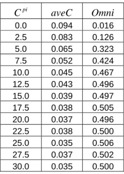
3.2 The strength of fixed lateral inhibition placed on the proximal compartment against average correlation and omnipotency score………..40
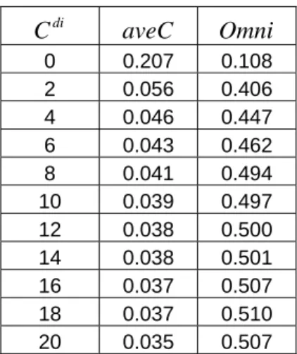
3.3 The strength of Anti-Hebbian plastic lateral inhibition placed on the distal compartment against average correlation and omnipotency score …..……..41
ix
LIST OF FIGURES
Figure
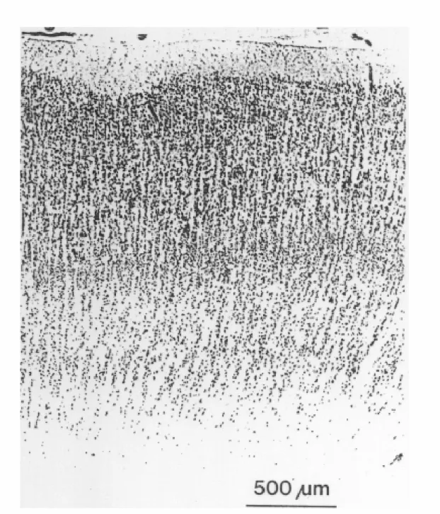
1.1 Histological section of primate somatosensory cortex………13
1.2 Local receptive field diversity in primary somatosensory cortex………...14
1.3 A hypothetical illustration of shuffled minicolumnar receptive field centers and macrocolumnar organization………..15
1.4 1994 Favorov-Kelly model………..16
2.1 Three-layer structure of somatosensory minicolumnar model………..28
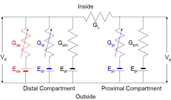
2.2 Neuron representing a minicolumn is modeled as a two-compartmental electrical circuit……….29
2.3 Coordinates of receptive field centers of thalamic units and stimulus strength as a function of time……….30
3.1 Receptive field centers of minicolumns before connection development……43
3.2 Color-coded skin field and minicolumns colored by the position of their receptive fields before connection development……….44
3.3 Histogram of correlations before connection development………45
3.4 Shuffled receptive field centers of minicolumns after connection development………..46
3.5 Color-coded skin field and minicolumns colored by the position of their receptive fields after connection development……….47
3.6 Histogram of correlations after connection development………...48
3.7 Trajectories of receptive field centers of minicolumns during connection development with optimal parameters and settings………49
3.8 Shuffled receptive field centers of minicolumns after connection development with optimal parameters and settings………50
settings………...51
3.10 Histogram of correlations after connection development with optimal parameters and settings………..52
3.11 Average correlation plotted against fixed lateral inhibition strength………….53
3.12 Omnipotency score plotted against fixed lateral inhibition strength………….54
3.13 Fixed lateral inhibition is extended to a radius of 2 minicolumns………..55
3.14 Average correlation plotted against Anti-Hebbian plastic lateral inhibition strength………..56
3.15 Omnipotency score plotted against Anti-Hebbian plastic lateral inhibition strength………..57
3.16 A nt i -H eb bia n p las t ic la t er al inh ibitio n is pla ce d in t he pr oxim a l compartment………..58
3.17 Average correlation plotted against longitudinal conductance………..59
3.18 Omnipotency score plotted against longitudinal conductance………..60
3.19 Orientation tuning plot 1...………...61
3.20 Orientation tuning plot 2………...………...62
4.1 Mutual fixed lateral inhibition between two neighboring cortical neurons with largely overlapped receptive fields………68
CHAPTER 1 INTRODUCTION
The cerebral cortex is the body organ whose task is, most fundamentally, to
process sensory information. This information enters the cortex via the thalamus in
its “raw” form, in which stimuli are reflected in the spatiotemporal patterns of
activities of the thalamic cells in an essentially isomorphic (photographic image-like)
and difficult to interpret manner. In the cortex this initial representation of the
sensory information undergoes a series of transformations in a more-or-less
hierarchical sequence of cortical areas, which extract and make progressively more
explicit the neural representation of the behaviorally significant information
(Bankman et al., 1990). The nature of these transformations and the neural
mechanisms that accomplish them remain poorly understood. This dissertation
investigates the first of these transformations in the somatosensory system, which
takes place in the input layer, or layer 4, of the cytoarchitectonically defined
Brodmann’s area 3b of the primary somatosensory cortex (SI). Area 3b receives
input primarily from cutaneous mechanoreceptors and responds to tactile stimuli.
Information from skin receptors is transmitted to the Ventral Posterior Lateral
(VPL) nucleus in the thalamus via synaptic relay in the Dorsal Column Nuclei (DCN)
of the brainstem. From VPL this information is delivered to neurons comprising layer
(i.e., areas 3a, 1, and 2). The information that flows from the skin via the thalamic
relay to the cortex is reflected in the receptive fields of somatosensory receptors and
DCN, VPL and cortical neurons. Receptive field of a neuron is the sensory area
within which a stimulus can evoke a response of the neuron. The receptive fields of
somatosensory receptors are very small and uniformly excitatory. Since the
receptive fields of the relay neurons are defined by the presynaptic afferent neurons
that converge on them, their receptive fields grow in size. In addition, inhibitory
interneurons participate and reshape the receptive fields of higher-level neurons to
have both excitatory and inhibitory subregions, which enhance the contrast between
stimuli. Although along the ascending somatosensory pathways each presynaptic
neuron has divergent presynaptic connections with multiple postsynaptic neurons,
and each postsynaptic neuron has convergent postsynaptic connections with
multiple presynaptic neurons, the topographic arrangement of receptive fields is
preserved (to varying degrees) in the thalamus and in the somatosensory cortex.
The excitatory and inhibitory regions of receptive fields can not only enhance
the contrast between stimuli, but also give rise to more complex feature-detecting
abilities of higher-order neurons. To illustrate on an example from the visual system,
the receptive fields of retinal bipolar and ganglion cells and thalamic neurons in the
3
a ring of light shining on the entire surround of its receptive field. The responses of
the OFF-CENTER cell are the opposite. Diffuse illumination on the entire receptive
field of either the ON-CENTER or OFF-CENTER cell will produce only weak
responses because the evoked excitation and inhibition cancel each other out
almost completely. Therefore, due to their ON-CENTER or OFF-CENTER receptive
fields, the bipolar cells, ganglion cells and neurons in the lateral geniculate nucleus
are capable of measuring local contrast in light intensity. However, neurons in the
primary visual cortex (V1) respond weakly to a beam of light but best to a bar of light
with a specific axis of orientation. Their receptive fields are no longer circular but
elongated, with the excitatory region in the middle flanked by the inhibitory regions
on one or both sides, or vice versa. The resulting rectilinear receptive fields enable
cells in the primary visual cortex to respond optimally to light stimuli with matching
geometrical characteristics – in this case a line, bar or edge – and axis of orientation.
Therefore the higher-order neurons in the primary visual cortex are capable to detect
a novel kind of feature: an edge with a specific axis of orientation. These receptive
fields result from the appropriate thalamocortical connection pattern: the excitatory
regions in the receptive fields of layer 4 cells in the primary visual cortex largely
overlap with the receptive fields of their input ON-CENTER thalamic neurons in the
lateral geniculate nucleus, and the inhibitory regions in the cortical receptive fields
coincide with the receptive fields of their OFF-CENTER thalamic neurons in the
lateral geniculate nucleus (see, for example, Miller et al., 2001). In addition, the
feed-forward inhibition from interneurons driven by the thalamus plays an important role in
directly from the thalamus. The feed-forward inhibition dominates the feed-forward
excitation in most non-preferred orientations. Only within a very narrow range around
the preferred orientation, the feed-forward excitation exceeds the feed-forward
inhibition. The feed-forward inhibition thus helps to further sharpen the orientation
tuning of layer 4 neurons.
The cerebral cortex is organized into vertical columns running through the
entire six layers of the cerebral cortex from the pial cortical surface to the white
matter (Mountcastle, 1978, 1997). This columnar organization is regarded as the
basic structural principle of the cerebral cortex. This columnar organization is
determined by intrinsic connectivity of the cerebral cortex, which is dominantly
vertical. The spiny stellate neurons, located in the input layer 4, are the principal
neurons receiving afferent input from the thalamus or other cortical areas. The
pyramidal neurons are located in almost every layer, except for layer 1, and they are
the principal output neurons. The axons of the spiny stellate neurons spread
vertically towards the surface of the cerebral cortex. Also both the apical dendrites
and axons of the pyramidal neurons are oriented perpendicular to the cortical
surface, thus parallel to the axons of the spiny stellate neurons, and forming vertical
bundles, which establish the anatomical basis of the vertical columns. Figure 1.1
5
functional unit of the cerebral cortex, which has been since supported by extensive
anatomical and physiological evidence (see for example a recent review by
Tommerdahl et al., 2005).
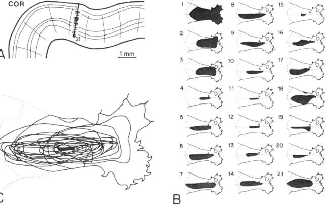
Receptive fields of neurons located in close proximity to each other in the
cortex are not uniform, but can vary prominently in their sizes, shapes, and positions
on the skin. Figure 1.2, adapted from Favorov and Diamond (1990), illustrates such
diversity in a typical near-radial microelectrode penetration of area 3b of a cat, in
which 21 neurons were isolated and their receptive fields mapped. Significant
differences in shape, size and skin position are evident in 21 individual receptive
fields, though there is a very small common area shared by all the 21 individual
receptive fields (see black region in the superimposed plot of the outlines of all 21
receptive fields in the left-bottom panel). Similarly diverse receptive fields among
neighboring cortical neurons can be found in the primate somatosensory cortex
(Powell and Mountcastle, 1959; McKenna et al., 1982; Iwamura et al., 1985; Favorov
and Whitsel, 1988a,b; and Favorov and Diamond, 1990), in the visual cortex (Hubel
and Wiesel, 1962, 1974a,b; Creutzfeldt et al., 1974; Albus, 1975a; Zohary et al.,
1994; Gochin et al., 1991; Fujita et al., 1992; and Gawne and Richmond, 1993), and
in the auditory cortex (Abeles and Goldstein, 1970).
Such diversity in receptive fields of neighboring cortical neurons is most
prominent when those neurons are located in different minicolumns. Figure 1.3
schematically illustrates this idea on hypothetical data. On the left, shown as black
dots are individual neurons in a Nissl-stained histological section of the primary
neurons are shown as black dots in a two-finger figurine on the right. According to
this figure, which summarizes experimental findings of Favorov and Whitsel (1988b),
Favorov and Diamond (1990) and Tommerdahl et al. (1993), as long as neurons are
located in the same minicolumn (e.g., neurons a-g in the figure), their receptive
fields are very similar to each other. On the other hand, when neurons are
compared across a sequence of minicolumns (e.g., neurons 1-30), their receptive
fields bounce back and forth randomly around a common center, forming a cluster.
Such seemingly random shuffling of receptive field centers is a characteristic of local
groups of minicolumns, which are separated by sharp boundaries, crossing which
shifts receptive fields to a new skin region. These sharp boundaries partition the
somatosensory cortex into a honeycomb-like mosaic, resulting in larger columnar
units named “segregates” (Favorov et al., 1987; Favorov and Whitsel, 1988a;
Favorov and Diamond, 1990). A segregate is approximately 0.3-0.6 mm in diameter
and consists of 60-80 minicolumns. The receptive fields of the minicolumns within a
segregate together cover an extended skin region, although receptive fields of most
minicolumns in a segregate overlap only minimally and, consequently, all together
they share only a very small skin region in common, called the segregate receptive
field center (see Figure 1.2). Segregate receptive field centers are arranged
7
responsive to light bar stimuli of all orientations from a particular region in the visual
field. In rodent primary somatosensory cortex, Woolsey and Van der Loos (1970)
discovered the “barrels” which are discrete structural and functional units that
receive and process input from individual “principal” facial whiskers. In general, such
larger-scale discrete vertical columnar units are called macrocolumns (Mountcastle,
1978). A macrocolumn is composed of minicolumns that share certain functional
properties. Macrocolumns are regarded as computational modules, each of which
receives specific input information, transforms that information, and sends the output
to other higher-level associative cortical areas. The anatomical basis of
macrocolumns is that minicolumns within the same macrocolumn share similar
thalamocortical afferent input connections.
Traditionally, since the macrocolumn has been regarded as a functional
module, the similarities among minicolumns within a macrocolumn have been
emphasized. However, as reviewed above, there exist prominent differences in
some of the functional properties among minicolumns within a macrocolumn, such
as for example diversity in exact receptive field positions on the skin. In order to
investigate the possible underlying mechanisms responsible for such diversity of
receptive fields of minicolumns within a macrocolumn and their potential significance
for the functional properties of the macrocolumn, Favorov and Kelly (1994a,b)
developed a computational model of a single macrocolumn as a set of 61
minicolumns.
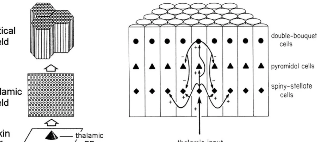
The model’s connectional architecture is shown in Figure 1.4. In it the
the cortex. The receptive fields of the thalamic neurons are circular and are
topographically arranged on the skin, thus resulting in a two-dimensional array on a
two-dimensional surface. The cortex in this computational model is composed of
regular hexagon-shaped macrocolumns, each macrocolumn is made up of 61
cylinder-shaped minicolumns, and each minicolumn is represented by three cortical
cells of three distinct types: a spiny stellate cell, a pyramidal cell and a double
bouquet cell. The spiny stellate cell receives excitatory afferent input from multiple
thalamic neurons and feed-forwards the excitation to the pyramidal cell and the
double bouquet cell within the same minicolumn, and to a smaller magnitude, to the
neighboring spiny stellate cells up to two minicolumns away. The double bouquet cell
inhibits only the pyramidal and spiny stellate cells of the immediately adjacent
minicolumns. The synaptic connections between the thalamic neurons and the spiny
stellate cells are plastic. The thalamocortical synaptic connection strengths are
initialized randomly and then adjusted according to the Hebbian Synaptic Plasticity
Rule until they are stabilized during the “developmental” stage in which the whole
thalamocortical network is trained by a long series of point stimuli on the
two-dimensional skin surface. All the other synaptic connection strengths are
predetermined and fixed throughout the simulation. In the following text, this
9
simulated neurons based on the 1994 Favorov-Kelly model in functional properties,
such as orientation tuning. The model cells can develop only very modest
orientation tuning, much weaker than that of real neurons in the primary
somatosensory cortex (Bensmaia et al., 2008).
The second limitation concerns the double bouquet cell, which is proposed to
provide fixed lateral inhibition in the 1994 Favorov-Kelly model. There are two
problems associated with the double bouquet cell. The first problem is that only in
primates double bouquet cells contact spiny-stellates (Casanova, 2005), which
renders the 1994 Favorov-Kelly model more specialized and less generic. The
second problem is that even in primates double bouquet cells cannot exert strong
enough inhibition on spiny stellate cells. The closer the inhibition is to the axonal
output part of a neuron, the more effective the inhibition is. Real double bouquet
cells synapse on dendrites of spiny stellate cells, which correspond to the distal
electrical compartment of the spiny stellate cells in the 1994 Favorov-Kelly model.
However, in the 1994 Favorov-Kelly model, fixed lateral inhibition is placed in the
proximal electrical compartment, which corresponds to the soma of spiny stellate
cells. Therefore, the double bouquet cell is not a good candidate for providing fixed
lateral inhibition in the 1994 Favorov-Kelly model.
In this dissertation work, we developed a computational system largely based
on the 1994 Favorov-Kelly model to simulate information processing in cortical layer
4 of a macrocolumn composed of minicolumns. Besides addressing the above two
limitations, we used this system to investigate the potential contribution of lateral
The first property is that the activities of neighboring cortical neurons are
essentially fully decorrelated. It is well known that neurons located in close proximity
to each other in cortical gray matter tend to have similar stimulus response
properties, and thus they tend to respond similarly to test stimuli. They are also
known to synchronize their spike discharges temporarily in response to some of the
test stimuli. However, despite such notable similarities, the response properties of
nearby cortical neurons are still quite diverse (as reviewed above), so that across
the full repertoire of stimulus patterns experienced in the individual’s regular life,
neighboring cortical neurons turn out to be essentially fully decorrelated in their response behaviors. That is, when compared across ethologically representative
sets of stimuli, responses of neighboring neurons in a cortical column are found
close to be statistically independent (Gawne and Richmond, 1993; Ghose et al.,
1994; Zohary et al., 1994; Gawne et al., 1996; Vinje and Gallant, 2000; Reich et al.,
2001).
The second property that we postulate for the layer 4 transform of its afferent
information might be defined as a “hidden information maximization” principle. To
explain, considering information coding abstractly, the same information can be
coded, or represented, in a set of information-carrying channels in a wide variety of
11
very complex (requiring highly nonlinear integration of the states of many channels).
The dedicated channel strategy is not practical because of its limited
representational capacity, compared to distributed codes, in which multiple
channels carry information about a given item together with information about some
other such items.
Among the distributed codes, the algorithmically simplest ones are those that
to extract particular information require only linear summation of the states of the
relevant channels. Such codes can be easily used by biological neurons, by linear
dendritic summation of their synaptic inputs. We can call this linear-summation type
of information representation “explicit.” In contrast, the codes that require
algorithmically complex (nonlinear) means of information extraction can be called
“implicit.”
Using this terminology, we can state that most of the information coming from
the outside world to the brain is represented only implicitly by the activities of
sensory receptors. Such “deeply hidden,” or “high-level,” information is also turns
out to be most important to situation comprehension and behavioral decision making.
The basic task of the sensory cortex is to convert the originally implicit
representations of behaviorally-significant information into algorithmically simpler –
explicit – representations suitable for behavioral decision making. This task is
accomplished by the cortex incrementally and requires participation of multiple
cortical areas.
Considered in this light, the task of layer 4 input transform might be expected
behaviorally-significant sensory information as possible. However, layer 4 of the primary
somatosensory cortex, as the first stage in sensory input transformation, might not
be in a position to anticipate which information items might be behaviorally
significant and therefore should be made more explicit. Instead, a more general
“omnipotency” strategy might be to make more explicit as much of the hidden sensory information as possible. Such an omnipotency strategy, referred to as
kernel-based methods, has been found highly successful in computational fields of
Machine Learning and Pattern Recognition (Vapnik, 1995; Schölkopf and Smola,
2002).
In developing our minicolumnar model of somatosensory cortical layer 4
network, we hypothesized that in order to achieve maximal omnipotence, the
neurons in layer 4 must be essentially decorrelated, which would require strong
lateral inhibition among them. In turn, lateral inhibition can bring about nonlinearity in
information transformation in cortical layer 4, which is necessary for extracting
hidden information. In the following chapters, we show that omnipotency,
decorrelation, inhibition, and receptive field shuffling do indeed go together and their
13
Figure 1.1. Histological section of primate somatosensory cortex.
Figure 1.2. Local receptive field diversity in primary somatosensory cortex.
15
Figure 1.3. A hypothetical illustration of shuffled minicolumnar receptive field centers and macrocolumnar organization.
Figure 1.4. 1994 Favorov-Kelly model.
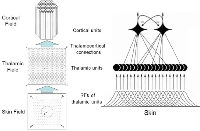
CHAPTER 2 METHODS
Our current computational system was developed primarily based on the
1994 Favorov-Kelly model (Favorov and Kelly, 1994a,b). The three-layer hierarchical
organization of the 1994 Favorov-Kelly model (Figure 2.1) was retained. It includes a
skin layer, a layer of thalamic units representing thalamic neurons, and a layer of
minicolumnar units representing layer 4 part of minicolumns. The skin is modeled as
a two-dimensional flat surface. The receptive fields of the thalamic units are
topographically arranged on the skin and have identical circular shape and identical
size. During computer simulations, multi-point stimuli are applied to the skin field.
The activity of each thalamic unit evoked by a single point stimulus is solely
determined by the distance between the position of the point stimulus and the
receptive field center of the thalamic unit in the skin field. The activity of each
thalamic unit evoked by a multi-point stimulus is calculated as the sum of the
activities of that thalamic unit evoked by each component point stimulus individually.
A minicolumnar unit receives excitatory afferent inputs from all the thalamic units.
Inputs from thalamic units and lateral inputs from surrounding minicolumnar units are
the driving forces to shape the receptive fields and functional properties of
minicolumnar units. The thalamocortical synaptic connections are plastic. The lateral
As in 1994 Favorov-Kelly model, a single macrocolumn is modeled as
composed of 61 minicolumnar units organized into a regular hexagon shape
structure (Figure 2.1). Each minicolumn is represented by a prototypical neuron that
is modeled as a two-compartmental electrical circuit (illustrated in Figure 2.2). Each
minicolumn inhibits its immediate neighboring minicolumns via fixed inhibitory lateral
connections and it also inhibits all other 60 minicolumns via Anti-Hebbian plastic
inhibitory lateral connections.
Both the excitatory thalamocortical afferent connections and the Anti-Hebbian
plastic inhibitory lateral connections are modifiable according to the Hebbian Rule
(Fyffe, 2005) in the “connection development” stage of computer simulations. The
correlation between the activity of a thalamic unit and the activity of a minicolumnar
unit is used to determine the strength of Hebbian excitatory thalamocortical
connection between them. The correlation between activities of two minicolumns is
used to determine the strength of the Anti-Hebbian plastic inhibitory lateral
connection between them. The strength of the fixed lateral inhibitory connections
between immediate neighboring minicolumns is constant and uniform.
In this newly developed computational system, the minicolumn-representing
neuron is modeled as a two-compartmental electrical circuit, illustrated in Figure 2.2.
19
placed on the distal compartment and the proximal compartment, respectively. In our
new system lateral excitation is excluded and two types of lateral inhibition are
placed on the distal compartment and the proximal compartment. In Figure 2.2, Gde
is the conductance of excitatory synapses on the distal compartment. Gdi and Gpi
are the conductances of inhibitory synapses on the distal compartment and the
proximal compartment, respectively. Gdm and Gpm are passive membrane
conductances of the distal compartment and the proximal compartment, respectively.
L
G is the longitudinal conductance connecting the distal compartment and the
proximal compartment. Ede is the reversal potential of excitatory synapses on the
distal compartment. Edi and Epi are the reversal potentials of inhibitory synapses on
the distal compartment and the proximal compartment, respectively. Edr and Epr are
resting membrane potentials of the distal compartment and the proximal
compartment, respectively. Vd and Vp are membrane potentials of the distal
compartment and the proximal compartment, respectively.
Computer simulation of the model is divided into two stages. The first stage is
the “connection development” or “self-organization” stage. Initially, the weights of
thalamocortical connections and the Anti-Hebbian plastic inhibitory lateral
connections are assigned randomly. Then the system is trained by applying
randomly picked multi-point stimuli to the skin. The reason that we chose to use
multi-point stimuli instead of single-point stimuli was to increase the complexity of
training patterns in order to explore the state space more extensively. The second
system.
The connection-development program updated the plastic connections after
every 1000 randomly generated 5-point stimuli. In response to each five-point
stimulus applied to the skin field, we calculated the instantaneous firing rate for each
minicolumn-representing neuron. First, we calculated the activity of every thalamic
unit evoked by each of the five points. The activity TH ij
F of the thalamic unit i evoked
by the single-point stimulus j was calculated as:
+ − = max(1 TH)
ij TH TH ij R D F F ,
where TH
Fmax = 1 is the maximal possible activity of a thalamic unit which could be
evoked by a single-point stimulus. Dij is the distance from the position of the point
stimulus j to the receptive field center of the thalamic unit i. TH
R is the radius of the
receptive field of a thalamic units and it was set to 3, as in 1994 Favorov and Kelly
model. The plus sign indicates the calculated value inside the parentheses should be
set to zero if it is negative. Next, the activity TH i
F of the thalamic unit i evoked by the
five-point stimulus was calculated as the sum of activities of the thalamic unit i
evoked by each of the five points individually:
∑
= 5 THij TH
i F
21
∑
= = 127 1 ) ( j TH j TH ij AFi f W F
F ,
where TH ij
W is the strength of the thalamocortical synaptic connection between the
thalamic unit j and neuron i. Next, the conductances of the excitatory and inhibitory
synapses on the distal compartment and the inhibitory synapses on the proximal
compartment were calculated according to the following differential equations:
∑
∑
+ − = + − = + − = k MC k pi pi i pi i j MC j di ij di di i di i AF i de i de i F C G G dt d F W C G G dt d F G G dt d μ μ μwhere MC j
F is the output activity of minicolumn j, μ is a time constant, di
C and pi
C
are scaling constants for inhibition in the distal and proximal compartments,
respectively, and di ij
W is the weight of the inhibitory connection from minicolumn j to
minicolumn i. These differential equations were solved numerically using Euler
method as follows:
∑
∑
Δ + Δ − = Δ + Δ + Δ − = Δ + Δ + Δ − = Δ + k MC k pi pi i pi i j MC j di ij di di i di i AF i de i de i t F C t t G t t t G t F W C t t G t t t G t F t t G t t t G ) ( ) / ( ) ( ) / 1 ( ) ( ) ( ) / ( ) ( ) / 1 ( ) ( ) ( ) / ( ) ( ) / 1 ( ) ( μ μ μ μ μ μThe time step Δt and time constant μ were set to 1 millisecond and 4 milliseconds,
respectively.
∑
kMC k
F denotes the summation of activities of immediately neighboring
minicolumns.
∑
jMC j di ij F
minicolumns. The membrane potential d
V of the distal compartment and the
membrane potential p
V of the proximal compartment are determined as follows:
) 1 ( ) 1 )( 1 ( ) 1 ( ) 1 )( 1 ( ) 1 ( + + + + + + = + + + + + + + + = pi L L pi di de L de p pi L L pi di de L pi de d G G G G G G G G V G G G G G G G G G V
where GL is the longitudinal conductance connecting the distal compartment and
the proximal compartment. The “activity,” in a form of an instantaneous firing rate,
MC i
F of the neuron representing minicolumn i is determined by its membrane
potential of the proximal compartment p
V : 3 3 ) ( 01 . 0 ) ( p p MC i V V F + =
At the end of each round of 1000 randomly chosen five-point stimuli, the plastic
connections were updated as follows:
+ + ⋅ + ⋅ − = ⋅ ⋅ + ⋅ − = )] , ( ) 1 [( ] )) , ( ( )) , ( ( ) 1 [( 2 MC j d i di ij di ij TH j d i TH j d i TH ij TH ij F V corr RM W RM W F V corr F V corr sign RM W RM W
RM is the rate of connection maturation, set to 0.1. sign() function outputs
positive or negative sign depending on the value inside the parenthesis. corr()
function calculates the correlation between given variables. Therefore, the synaptic
23
by the correlation between the output activity of the presynaptic minicolumnar unit
and the distal membrane potential of the postsynaptic minicolumnar unit. These
correlations were computed over the values of the variables taken on the 50th time
step of the network’s responses to 1000 randomly chosen 5-point skin stimuli. In
order to prevent the activities of minicolumns from becoming excessively large or
invariably zero, we normalized the thalamocortical connection weights of each
neuron by summing all of its thalamocortical connection weights and then dividing
each thalamocortical connection weights by this sum. Finally, to ensure that all
neurons will have the average output activity in response to 5-point stimuli close to a
certain desired value (chosen to be 0.075), the normalized thalamocortical
connection weights were further scaled by 0.075/FSSi, where FSSi is the average
activity of neuron i across the previous 1000 stimuli.
After the excitatory thalamocortical afferent connections and the Anti-Hebbian
plastic inhibitory lateral connections were fully developed, we characterized the
system’s performance by computing the average distance between receptive field
centers of immediate neighboring minicolumns and the average correlation between
activities of all pairs of minicolumns in response to 1000 randomly chosen 5-point
stimuli. We then ran an omnipotency test.
As the system was developing its plastic connections, the trajectories of the
receptive field centers were displayed in real time to monitor the progress of the
connection development. When the system reached the steady state, the receptive
field centers stopped traveling. Then we generated a “receptive field shuffling” plot
straight lines to demonstrate their relative positions and how well they shuffled. The
less the lines crossed one other, the less prominently the receptive field centers of
minicolumns within the same macrocolumn shuffled. The average distance between
receptive field centers of adjacent minicolumns was calculated to indicate to what
extent the receptive field centers of immediate neighboring minicolumns were
separated. The greater the average distance was, the more spread out the receptive
field centers were and the more they shuffled. We also produced a color-coded map
to demonstrate the positions of receptive field centers of the minicolumns on the skin.
Different colors were used to distinguish different regions of the skin field. The
receptive field centers were represented by white dots scattered in the color-coded
skin field. In the accompanying color-coded honeycomb-like macrocolumn image,
each of the 61 minicolumns was colored depending on the color of the region in the
skin field where its receptive field center was located. A pattern of gradual transition
or systematic alternation in color of 61 minicolumns within the same macrocolumn
would indicate a somatotopic map. We expect to observe each minicolumn in a
distinctive color and the colors of neighboring minicolumns referred to very different
regions of the skin field.
In order to assess how well the 61 minicolumns within the same macrocolumn
25
and the histogram of the correlations demonstrated that the percentages of high
correlations were nearly 0 and most correlations were negative or close to 0.
The network with fully developed thalamocortical and anti-Hebbian inhibitory
connections was evaluated for its “omnipotency,” defined as the capacity to
represent any arbitrarily defined nonlinear features of stimulus patterns. Any such
stimulus feature can be defined as a function over the stimulus/input space. Thus,
our omnipotency test involves defining an arbitrary test function T(S) on an arbitrarily
chosen set of 5-point stimuli S1 … Sn. Typically in our studies we use n = 20. The
test function T(S) is given a value of 0 or 1 on each of the n test stimuli, such that for
each thalamic unit the correlation coefficient between its responses to these n test stimuli and T(S) is equal to zero. This means that this test function – or stimulus
feature – is “hidden” at the level of the thalamic units; i.e., it is represented only
implicitly in the thalamic layer and cannot be extracted (i.e., made explicit) by any
linear summation of the activities of the thalamic units.
Next, we compute the responses F1MC...F61MCof all 61 minicolumns to each of
the n test stimuli. As a rule, because the minicolumnar output is a nonlinear
transform of the thalamic input, the correlation coefficient between responses of any
given minicolumn to the test stimuli and T(S) is most likely to be non-zero. The
question is: Will the test function T(S) be represented explicitly – and to what degree
– by outputs of the 61 minicolumns? How well would a hypothetical neuron in the
other cortical layers be able to represent function T(S) by computing a weighted sum
of outputs of the 61 minicolumns? Of course, if we used error-correction learning,
test stimuli (since the number of its input channels, 61, is much larger than the
number of training samples, n = 20). However, assuming that cortical neurons do not
use error-correction learning, but Hebbian learning, our hypothetical neuron will not
be as successful. To approximate Hebbian limitations, for each minicolumn i we
compute the correlation coefficient rT,i between T(S) and the responses of that
minicolumn to the n test stimuli. Now we can compute the output of the hypothetical
neuron in response to a given test stimulus s as:
). ( ) ( 61 1
, F s
r s
F iMC
i i T ⋅
=
∑
=How well will F(S) approximate T(S) on test stimuli S1 … Sn? We measure it
by computing the correlation coefficient rT,F between F(S) and T(S), giving us the
upper bound for the ability of the outputs of the 61 minicolumns together to linearly
represent the test function T(S).
Finally, to obtain a general estimate of this ability to represent arbitrary test
functions, we repeat this test study 100 times, each time using different test
functions T(S) defined on different sets of test stimuli S1 … Sn, and use the average
squared correlation coefficient 2 ,F T
r as our measure of representational omnipotency of the studied minicolumnar network.
27
straight line. The activities of minicolumns evoked by those line stimuli in every
orientation were recorded and displayed in two different ways. One was to simply
plot the activity as a function of stimulus orientation. The other was to draw every
line stimulus in its proper orientation, but with its length determined by the activity of
Figure 2.1. Three-layer structure of somatosensory minicolumnar model.
29
Figure 2.3. Coordinates of receptive field centers of thalamic units and stimulus strength as a function of time.
CHAPTER 3 RESULTS
We first establish that the new model can successfully reproduce the shuffled
receptive fields of minicolumns similar to those obtained by the 1994 Favorov-Kelly
model. As illustrated in Figure 3.1 – 3.6, the new model was not only able to
reproduce the shuffled receptive fields of minicolumns, but also improved
decorrelation among minicolumns.
The network’s starting state before the development of thalamocortical
connections and its stable state after the development are shown in Figures 3.1 –
3.6. Since there were significant modifications made to the 1994 Favorov-Kelly
model, we used equivalent rather than identical parameters in our simulation to
approximate the old results. All the parameters are documented in Tables 3.1 – 3.4,
if not mentioned otherwise. Since the thalamocortical connections were prescribed
randomly initially, the receptive field centers of 61 minicolumns within the same
macrocolumn are randomly dispersed within a relatively small skin region with an
average distance of 1.628 units between immediate neighboring minicolumns
(Figure 3.1 – 3.2). In the circular color-coded skin map (Figure 3.2), most of the
receptive field centers are scattered more towards the center of the skin. In the
corresponding honeycomb shaped macrocolumn, there was no systematic
thalamocortical connections reached the steady state, the receptive field centers of
the 61 minicolumns within the macrocolumn become distributed in a much larger
region with an average distance of 4.269 units between immediate neighboring
minicolumns (Figure 3.4). Figure 3.4 demonstrates the relative positions of receptive
field centers with lines connecting the immediate neighboring minicolumns. It was
observed, interestingly, that the image is composed of numerous triangles rotating
from and superimposed on each other. The circular color-coded skin map clearly
demonstrates that the receptive field centers are scattered more towards the skin
margins, resulting in a vast empty space at the center of the skin field (Figure 3.5).
Although the new model did successfully reproduce the shuffled receptive
fields of the 61 minicolumns, the patterns of the shuffled receptive field centers were
different between the new model and the 1994 Favorov-Kelly model (Favorov and
Kelly, 1994 a). It was not only due to the non-identical parameters but also, more
importantly, due to the modifications made to the 1994 Favorov-Kelly model. In short,
the new model does not have parasynaptic influences from surrounding
macrocolumns imposed on the 61 minicolumns within the central macrocolumn
because only the central macrocolumn is modeled now. In the 1994 Favorov-Kelly
model, the receptive field centers of the 61 minicolumns within the central
33
less distributed evenly throughout the skin field. However, in this new model, there
are no such surrounding macrocolumns and parasynaptic influences. It is the strong
fixed lateral inhibition between immediate neighboring minicolumns that is primarily
responsible for driving the receptive field centers of all 61 minicolumns away from
the center of the skin field. Because of the repulsive nature of the inhibition, the
strong fixed lateral inhibition between immediate neighboring minicolumns tends to
drive the receptive fields of minicolumns as far apart as possible. The above
explanation is confirmed by the pattern of color alternation of the 61 minicolumns in
the left panel of Figure 3.5. For example, the minicolumn at the upper rightmost
corner of the macrocolumn is color-coded in vivid-blue, but two of its three
immediate neighboring minicolumns are in brown and the third one is in green. From
the corresponding color-coded skin field, the vivid blue is almost opposite to the
brown and nearly opposite to the green.
Another undesired feature produced by the new model is that although the
immediate neighboring minicolumns have very different receptive fields, more distant
minicolumns share similar receptive fields. As illustrated in Figure 3.5, taking the
minicolumn at the upper rightmost corner of the macrocolumn as an example again,
there are two minicolumns color-coded in dark-blue within a radius of two
minicolumns.
The existence of similar receptive fields among non-adjacent minicolumns
suggests the existence of high correlation between their activities evoked by the
same point stimuli, which is confirmed by Figure 3.6 which shows the histogram of
the 5-point stimuli. In contrast to the histogram of the correlations of the starting state
(Figure 3.3), which was almost flat and evenly distributed ranging from -0.25 to +1,
the histogram of the correlations of the stable state indicates that during computer
simulation a significant number of pairs of minicolumns were indeed decorrelated,
resulting in a significant increase in the percentage of correlations close to 0.
However, the percentage of the correlations with value 1 also increased and
therefore confirmed the existence of highly correlated pairs of minicolumns, which is
undesirable since we hypothesized that minicolumns in the cerebral cortex should
be essentially decorrelated and independent from each other in order to reduce
redundant information and achieve the maximal omnipotency in information
transformation. In turn, the results obtained from the omnipotency test indicates that
there was no significant improvement over the omnipotency and the omnipotency
scores were nearly zero for both the starting state and the steady state, which
suggest that the new model needs parameter optimization.
After searching systematically through the parameter space, we narrowed
down the number of critical parameters to 3 that maximize the network’s
omnipotency. Figures 3.7 – 3.10 illustrate the trajectories of minicolumnar receptive
field centers during the optimal development (Figure 3.7), the shuffled receptive field
35
experiments. The receptive field centers of neighboring minicolumns were dispersed
in a more complex pattern rather than the “zigzag” and the “triangles” (Figure 3.8).
The pattern of the color alternation of the 61 minicolumns within the same
macrocolumn represented more diversity and fewer stereotypes (Figure 3.9). In the
histogram of the correlations, the percentage of the correlations with values close to
1 was zero and the majority of the correlations were close to 0. The overall profile of
the histogram was closer to a normal distribution centered around 0 (Figure 3.10).
The average correlation and omnipotency score were improved to 0.039 and 0.497,
respectively.
We further investigated the contributions of the three critical parameters to
this newly developed minicolumnar model individually, focusing on decorrelation and
omnipotency. The results are illustrated in Figure 3.11 – 3.18.
First, we assessed the importance of the fixed lateral inhibition, which was
included in both the 1994 Favorov-Kelly model and the new model. We varied the
strength of the fixed lateral inhibition, ranging from 0 to 30, while setting all other
parameters to the optimal values (Figure 3.11 – 3.12). The average correlation did
clearly show the trend of descending and stabilizing roughly after the strength was
more than 15, which was the optimal parameter we chose for the strength of the
fixed lateral inhibition. Correspondingly, the omnipotency score increased gradually
from almost 0 to 0.5 and became saturated after the strength was more than 15.
Figure 3.11 – 3.12 revealed that the stronger the fixed lateral inhibition, the lower the
average correlation and the higher the omnipotency score. But the overall
Next, we kept all the parameters and settings the same as those in the
optimal condition, but extended the radius of the fixed lateral inhibition to 2
minicolumns. The results are illustrated in Figure 3.13. There was not much
difference in terms of the shuffled receptive fields except that the receptive field
centers were distributed more towards the center of the skin field in this trial, while
the receptive field centers were more spread out under the optimal condition. The
histogram of the correlations was less ideal than the one observed with the optimal
condition and the percentage of high correlations increased. Although the average
correlation remained nearly zero, the omnipotency score dropped significantly from
0.497 under the optimal condition to 0.140 in this trial! These results suggest that
this neural network achieves its best performance with the fixed lateral inhibition
restricted to immediate neighboring minicolumns.
Next, we evaluated the importance of the Anti-Hebbian plastic lateral
inhibition, which was introduced in this new model. Again, we retained the optimal
parameters and settings except for varying the scaling constant controlling the
strength of the Anti-Hebbian plastic lateral inhibition, ranging from 0 to 20 (Figures
3.14 – 3.15). Both the average correlation and the omnipotency score showed sharp
transitions from 0 to 2 but the overall trends were similar to the ones we observed in
37
compartment, while retaining all the other optimal parameters and settings. The
results are illustrated in Figure 3.16. Once again, the omnipotency score dropped
significantly from 0.497 under the optimal condition to 0.139 in this trial, which
suggested that it was critical to place the Anti-Hebbian plastic lateral inhibition on the
distal compartment.
Next, we investigated the importance of the longitudinal conductance. The
results are illustrated in Figures 3.17 – 3.18, which clearly demonstrate that the
larger the longitudinal conductance, the higher the average correlation and the lower
the omnipotency score. Therefore, the smallest possible value of 2 was determined
to be the optimal value for the longitudinal conductance. The longitudinal
conductance connecting the distal compartment and the proximal compartment
controlled the influence imposed from one compartment on the other. Zero
longitudinal conductance separated the two compartments completely and
excessively large longitudinal conductance made the two compartments behave
essentially equivalent to one compartment. An effective two-compartment model is
necessary to the functioning of the newly developed minicolumnar model.
Separating the excitatory inputs (thalamic afferent inputs) from the fixed lateral
inhibitory inputs by placing them on different compartments helps to make them
more effective in the development of the thalamocortical connections and their
functional properties. Therefore, the smallest possible longitudinal conductance was
critical to the success of this newly developed minicolumnar model.
Lastly, in order to test the robustness of our newly developed minicolumnar
and compared with the published results based on the 1994 Favorov-Kelly model in
Figures 3.19 – 3.20. In Figure 3.19, although in the previous model we observed
differential responses of an example minicolumn to a vertically-oriented bar stimulus
and a horizontally oriented bar stimulus, the difference was not very big: the bar
stimulus in the non-preferred orientation (horizontal) still evoked strong response.
However, in the new model, most of the minicolumns are sensitive to narrow ranges
of stimulus orientations. A sharp peak in orientation tuning suggests that the
minicolumn responds actively only when the bar stimuli were closely aligned with its
preferred orientation. Figure 3.20 demonstrates the preferred orientations in an
alternative way. The results of orientation tuning obtained in the new model are
39
Index RM GL Cde Cpi Cdi # aveD aveC Omni Figure
1 0.1 2 0.05 2 0 10 1.628 0.324 0.030 3.1 - 3.3 2 0.1 2 0.05 2 0 200 4.269 0.200 0.055 3.4 - 3.6
3 0.1 2 0 15 10 200 5.120 0.039 0.497
3.7 - 3.10, 3.13, 3.16, 3.19, 3.20
Table 3.1. Parameters used in simulations and summary of results. RM (Rate of Maturation), L
G (Longitudinal Conductance), de
C (the strength of the lateral excitation placed on the distal compartment), Cpi (the strength of the fixed lateral inhibition placed on the proximal compartment), di
C (the strength of the Anti-Hebbian plastic lateral inhibition placed on the distal compartment), # (the number of connection updates), aveD (the average distance between the receptive field centers of immediate neighboring minicolumns in the skin field), aveC (the average correlations of activities of all 1830 pairs of minicolumns), Omni (the omnipotence score of the minicolumnar network or the macrocolumn).
pi
C aveC Omni
0.0 0.094 0.016 2.5 0.083 0.126 5.0 0.065 0.323 7.5 0.052 0.424 10.0 0.045 0.467 12.5 0.043 0.496 15.0 0.039 0.497 17.5 0.038 0.505 20.0 0.037 0.496 22.5 0.038 0.500 25.0 0.035 0.506 27.5 0.037 0.502 30.0 0.035 0.500
Table 3.2. The strength of fixed lateral inhibition placed on the proximal compartment against average correlation and omnipotency score.
41 di
C aveC Omni
0 0.207 0.108 2 0.056 0.406 4 0.046 0.447 6 0.043 0.462 8 0.041 0.494 10 0.039 0.497 12 0.038 0.500 14 0.038 0.501 16 0.037 0.507 18 0.037 0.510 20 0.035 0.507
Table 3.3. The strength of Anti-Hebbian plastic lateral inhibition placed on the distal compartment against average correlation and omnipotency score.
L
G aveC Omni
2 0.039 0.497 4 0.044 0.462 8 0.049 0.423 16 0.057 0.368 32 0.062 0.299 64 0.065 0.271 128 0.068 0.245 256 0.069 0.234 512 0.070 0.229 1024 0.070 0.226 2048 0.070 0.225
Table 3.4. Longitudinal conductance against average correlation and omnipotency score.
43
Figure 3.1. Receptive field centers of minicolumns before connection development.
Figure 3.2. Color-coded skin field and minicolumns colored by the position of their receptive fields before connection development.
45
Figure 3.4. Shuffled receptive field centers of minicolumns after connection development.
47
Figure 3.5. Color-coded skin field and minicolumns colored by the position of their receptive fields after connection development.
49
51
53
55
Figure 3.13. Fixed lateral inhibition is extended to a radius of 2 minicolumns.
57
Figure 3.16. Anti-Hebbian plastic lateral inhibition is placed in the proximal compartment.
59
61
Figure 3.19. Orientation tuning plot 1.
Figure 3.20. Orientation tuning plot 2.
CHAPTER 4 DISCUSSIONS
In this dissertation work, we developed a dynamic system to approximate the
layer 4 cortical network based on the 1994 Favorov-Kelly model. We simplified the
original model, placing emphasis on lateral inhibition. With this setup, we
successfully reproduced some characteristic features observed in real cortical
networks, such as shuffled receptive fields and emergence of prominent orientation
tuning. After numerous trials with a large variety of parameter settings, we finally
narrowed down the number of critical parameters to 3. These parameters were: (1)
the strength of the fixed lateral inhibition applied on the proximal compartment, (2)
the existence of the Anti-Hebbian plastic lateral inhibition imposed on the distal
compartment, and (3) the small longitudinal conductance between the proximal
compartment and the distal compartment of the modeled minicolumn-representing
neuron. Under the optimal condition, defined by the maximal omnipotence in the
neural network, the system achieves nearly zero average correlation between any
pair of its neurons, prominent receptive field shuffling, and well-developed
higher-level feature sensitivities.
The reason why the two-compartment design of modeled neurons was
necessary to the successful functioning of the system is as follows. Since the system
in the real cortical neurons and the characteristics of the model neuron were
determined at least in part by its thalamocortical connections, the lateral inhibition
must exist among the model neurons because of its influence on the development of
the thalamocortical connections. The existence of the lateral inhibition among the
model neurons forces each of them to develop different sets of thalamocortical
connections, resulting in receptive field positional heterogeneity. However, the
development of the thalamocortical connections primarily follows the Hebbian Rule.
If we adopted a one-compartment neuron model, the thalamocortical connections of
a neuron would continue to change until its excitatory thalamic input is balanced with
its inhibitory lateral input. At its full development, the excitation would cancel out the
inhibition completely. Therefore, in a one-compartment model, the development of
the thalamocortical connections following the Hebbian Rule eventually neutralizes
the impact of the lateral inhibition in shaping the properties of the output. But by
adopting a two-compartment model and separating the excitatory input from the
inhibitory lateral input, a win-win situation could be achieved. In order to approximate
real cortical neurons, the excitatory thalamic afferent input was placed on the distal
compartment and the inhibitory lateral input was arranged on the proximal
compartment. The influence imposed on one compartment from the other
65
excitatory thalamic afferent input, by the state of the proximal compartment,
dominated by the inhibitory lateral input. Therefore, with a small enough longitudinal
conductance between the two compartments, the two-compartment model can
satisfy our design requirements for the model neuron. That is, in the distal
compartment, the thalamocortical connections were developed following the
Hebbian Rule based on the correlation of the activities of the presynaptic cell and
the postsynaptic cell; meanwhile, in the proximal compartment, the lateral inhibition
was predominant and capable of shaping the functional properties of the model
neuron.
Results of computer simulations of the model presented in Chapter 3
demonstrate the importance of the lateral inhibition in improving the performance of
the neural network in decorrelation and omnipotence. But why the fixed lateral
inhibition had to be placed on the proximal compartment and restricted locally
between the immediate neighboring neurons, while the Anti-Hebbian plastic lateral
inhibition had to be placed on the distal compartment and link all pairs of
minicolumns in the macrocolumn? First of all, the closer the inhibitory input is to the
output, the more effective the inhibition is. The fixed lateral inhibition between two
immediate neighboring minicolumns could sculpt their receptive fields to certain
nonlinear features. For example, as illustrated in Figure 4.1, we assumed that the
thalamocortical connections of two hypothetical neurons had already reached the
steady state and the profile of their receptive fields in a unidimensional state space is
gaussian. In addition, these two neurons have largely overlapping receptive fields. If
gaussian profiles (shown by the red dashed line and the blue dashed line,
respectively, in Figure 4.1). However, if there was fixed lateral inhibition between
them, their receptive fields would be significantly altered, as indicated by the red
solid line and the blue solid line, respectively, in Figure 4.1, and their receptive field
profiles are no longer gaussian. A nearly complete inhibitory region is produced
between the excitatory regions of these two neurons, thereby creating a new feature
sensitivity.
The Anti-Hebbian plastic lateral inhibition between all pairs of the model
minicolumns helps to shuffle the receptive fields of the minicolumns across the entire
macrocolumn more thoroughly. As pointed out in Chapter 3, with the fixed lateral
inhibition between immediately neighboring minicolumns alone, the shuffled
receptive field centers of minicolumns were distributed in a “zigzag” pattern and
there were pairs of minicolumns which were highly correlated in response to skin
stimuli, resulting in lower performance in omnipotence. With the assistance from the
Anti-Hebbian lateral inhibition between all pairs of minicolumns, they all become
more or less decorrelated. Because the receptive field of a minicolumn was
determined primarily by the thalamocortical connections, the Anti-Hebbian plastic
lateral inhibitory input was placed on the distal compartment together with the