5310.pdf

Continuum-atomistic algorithms for dendritic formation

Gregory Herschlag

A dissertation submitted to the faculty of the University of North Carolina at Chapel Hill in partial fulfillment of the requirements for the degree of Doctor of Philosophy in the Department of Mathematics.

Chapel Hill 2013

Approved by

Sorin Mitran

M. Gregory Forest

Laura Miller

Rene Lopez

ABSTRACT

GREGORY HERSCHLAG: Continuum-atomistic algorithms for dendritic formation (Under the direction of Sorin Mitran)

Nanoscale patterning of materials at scales of less than 20nm remains a challenging

problem. Standard techniques, such as lithography, rely on electron and photon beams

to shape materials, yet these methods are difficult to employ at the sub 50nm scale. We

consider the possibility of employing natural interface instabilities during solidification

in order to reliably produce desirable structures. Existing continuum methods for

com-plicated materials may break down at these scales, while direct atomistic simulation is

computationally infeasible. The primary objective of the thesis is to develop methods

ca-pable of efficiently resolving the atomistic computations which may eventually be solved

concurrently with continuum scale approaches. In the present work we develop atomistic

algorithms to furnish closures for continuum methods. We develop novel molecular

tech-niques capable of resolving detail only about an interface with non-periodic boundaries

and accelerated by GPUs. The new algorithms provide a method to determine interfacial

dynamics based on local curvature, employing wedge shaped domains. These dynamics

lead to continuum closures which are used to determine necessary physical parameters

ACKNOWLEDGEMENTS

I would like to thank my advisor, Sorin Mitran, for his patience in teaching me

structure and planning, Greg Forest for his guidance, Laura Miller for giving me my

first taste of research, and my parents for their constant support. I am grateful to UNC

through which I have developed many friends and colleagues who have helped me grow

TABLE OF CONTENTS

LIST OF TABLES . . . vii

LIST OF FIGURES . . . viii

Chapter 1. Material design for interfacial growth phenomenon . . . 1

1.1. A brief survey of material design . . . 1

1.2. An outline for dendrite formation upon solidification . . . 6

2. Existing continuum solidification models . . . 9

2.1. Sharp interface models . . . 9

2.1.1. The Gibbs-Thomson relationship . . . 11

2.1.2. Algorithms for sharp interface methods . . . 21

2.1.3. Assumptions and limitations . . . 27

2.2. Phase field models . . . 28

2.2.1. Algorithms for phase field methods . . . 30

2.2.2. Assumptions and limitations . . . 31

3. Molecular dynamics and applications to solidification . . . 34

3.1. Statistical mechanics . . . 37

3.1.1. Common ensembles . . . 37

3.2. Hamiltonian dynamics . . . 41

3.2.1. Hamiltonian molecular dynamic algorithms . . . 42

3.2.2. Hamiltonian conservation of phase space . . . 44

3.3.1. The virial theorems to derive molecular temperature and pressure 46

3.3.2. NVT equations . . . 49

3.3.3. NPT equations . . . 50

3.3.4. Numerical integration of the NVT and NPT equations . . . 52

3.4. Closing the Gibbs-Thomson equation . . . 53

3.4.1. Determining density and latent heat . . . 53

3.4.2. Determining the curvature closure coefficient . . . 53

3.4.3. Determining the velocity closure coefficient . . . 60

3.5. Discussion . . . 62

4. Finite domain molecular dynamics with non-periodic boundaries . . . 63

4.1. The Langevin equation . . . 64

4.1.1. The classical Langevin equation . . . 64

4.1.2. The generalized Langevin equation . . . 66

4.2. Other existing non-periodic boundary methods . . . 71

4.3. A novel method for non-periodic boundaries . . . 74

4.3.1. Transition equations . . . 74

4.3.2. Closing the equations . . . 77

4.3.3. The numerical implementation . . . 81

4.3.4. Results . . . 84

4.3.5. Discussion . . . 90

4.4. A novel barostat without altered particle dynamcis . . . 92

5. Interface dynamics . . . 97

5.1. Details of previous methods . . . 98

5.2.2. Curved domains . . . 104

5.3. Effects on solidifying structures . . . 107

5.3.1. Solidifying argon . . . 114

6. Discussion and Future directions . . . 120

6.1. Summary . . . 120

6.2. Future directions . . . 121

LIST OF TABLES

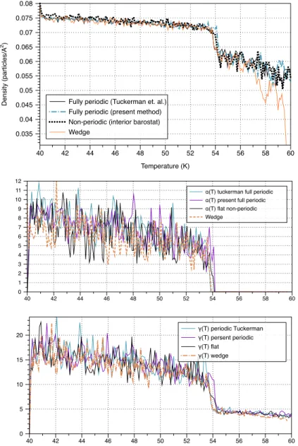
Table 4.1. Solid and liquid dilatation rates along with phase change temperature for all algorithms . . . 89

Table 5.1. Velocity closure coefficient of argon . . . 103

Table 5.2. Velocity of the front vs temperature in two wedge shaped domains . . 107

LIST OF FIGURES

1.1. Figure of nano-patterns on butterfly wings . . . 3

1.2. Physical outline of the mechanism behind solar cells . . . 4

1.3. Organization of the bulk-heterojunction . . . 5

3.1. Cleaving method to determine interfacial surface energy . . . 54

3.2. Work on the system during the cleaving method . . . 56

4.1. Chi-squared test for the distribution on a crystalline solid . . . 86

4.2. Correlations between velocity and mean position . . . 86

4.3. The mean virial gives incorrect NPT dynamics . . . 87

4.4. Statistical comparison of the new method with the periodic method . . . 88

4.5. Comparison of equilibrated and non-equilibriated wedge shaped domains . . 95

4.6. Large barostat frequencies may lead to accurate dynamics when compared to periodic simulations . . . 96

5.1. Solidification with imposed rate . . . 98

5.2. Solidification of argon for different thermo and barostat weights . . . 102

5.3. Solidification of argon for for the non-periodic, rectangular geometry . . . 103

5.4. Solidification of argon for for the non-periodic, wedge shaped geometry . . . . 106

5.5. Parameter sweep; increasing velocity closure coefficient with zero curvature closure coefficient. . . 109

5.6. Parameter sweep; increasing velocity closure coefficient with non-zero curvature closure coefficient. . . 110

5.7. Parameter sweep; increasing velocity closure coefficient with decreased latent heat and zero curvature closure coefficient. . . 110

5.8. Initial conditions in the planar solidification problem . . . 111

5.9. Demonstration of planar fingering . . . 112

5.11. Demonstration of no planar fingering . . . 113

5.12. Second demonstration of planar fingering . . . 113

5.13. Large undercooling of 10K in the liquid region of argon is unable to form dendrites at the 20nm scale. . . 117

5.14. Dendritic structure formation of argon. . . 117

5.15. A parameter sweep over the velocity and curvature closure coefficients for solidifying argon . . . 118

CHAPTER 1

MATERIAL DESIGN FOR INTERFACIAL GROWTH PHENOMENON

1.1. A brief survey of material design

The long-standing recognition that molecular arrangements and mesoscale structures

determine bulk material properties has led to the goal of gaining control over these

small scales to enable the design and fabrication of new materials. Conventionally, this

has been a process of trial and error: invent or select a material, allow it to undergo

a particular process and inquire into resulting macroscopic properties. Endeavors in

metallurgy have led to historically significant advances as well as recent insights and novel

material designs. For example, metals were strengthened by the addition or reduction

of impurities during fabrication; in one such instance of this process, ancient Damascus

sabers underwent a manufacturing process which embedded carbon nanotubes in the

weapons, leading to sharper and stronger blades [116]. Strong alloys also resulted from

this process; steel, for example, is produced by removing carbon impurities from melted

iron ore, and then alloying the metal with elements such as nickel or magnesium [82].

The processing of a material may also significantly change its properties, and Japanese

sword makers have long known that folding steel leads to more robust katanas [142]. The

metallurgical revolution continues to this day with advances in biologically unobtrusive

alloys used for surgical and dental implants [97], advances in annealing treatments for

heat resistant castings [11], and much more [105].

This approach of trial and error has also led to the polymer revolution in which

newly invented polymers have lead to a plethora of invention. Lead primarily by

Wal-lace Carothers of E. I. du Pont de Nemours and Company (DuPont), chemists began

proved remarkably useful, and have since become household names including neoprene,

mylar, nylon, teflon and vinyl. The processes to manufacture these polymers into

de-sirable bulk materials nearly always involve some combination of annealing (heating) a

polymer blend, pressing or stretching the material, or allowing the polymer to form a

thin film. For example, Arnold Miller Collins and Wallace Carothers discovered the

syn-thetic rubber neoprene by the purfication of divinyl acetylene in the presence of cuprous

chloride via a careful process of heating [48]. Mylar, which is stretched polyethylene

terephthalate (PET), is formed via a process that requires heating and stretching a thin

film [114]. Kevlar, invented by Stephanie Kwolek, is formed by extracting a mixture

of poly-p-Phenylene-terephthalate and polybenzamide from a spinneret, forming a fiber

with extremely high tensile strength [30]. In summary, the field of material fabrication

has been an enormously successful endeavor.

This success has lead to ever widening methodologies and approaches to design and

understand new materials. In addition to the chemical and manufacturing approaches

described above, computational simulations seek to provide insights toward gaining

con-trol over the microscopic scale in order to produce desirable properties at meso or macro

scales. Instead of starting with a microscopic material and then testing its macroscopic

properties, the framework is shifted: given desirable macroscopic properties, we search

for microscopic configurations that are able to produce these desirable properties. This

is a challenging problem and requires detailed mathematical models that span multiple

scales, along with numerical tools that are able to accurately capture desired

observ-ables, kinetics, and bulk properties. Perhaps the most prevalent method in material

design is density functional theory (DFT) [53]. In terms of bulk properties, DFT has

lead to improvements in alloy designs in titanium [68] and steel [54]. In [68], the Young’s

modulus was estimated by slight deformations in a body centered periodic cube (bcc)

composed of titanium and a variable second element; the authors were able to classify

and quantify structures which had greater tensile strength than pure bcc titanium which

new materials Gum Metals TM_{. DFT is also commonly used to determine jump rates for}

surface catalysis [117]; these reaction rates are then employed in kinetic Monte Carlo

simulations to determine the utility of different types of material for surface catalysis,

enabling for the optimization of surface type based on rates of catalysis. As a third, but

by no means exhaustive, example, DFT calculations were used to propose tetragonal iron

cobalt alloys which have highly desired uniaxial magnetic anisotropy along with a high

saturation magnetization; the new material may prove useful in improving the recording

density of hard drives [22].

In addition to DFT, an array of continuum models, stochastic, and molecular models

have enabled advancements in material design. For example, continuum models are

used to test and and simulate discovered materials and models have been used to stress

test airplanes, bridges and buildings given strength estimates of component parts (for

example [47], [94], and [158] respectively). Stochastic methods have been used effectively

Figure 1.1. Figure take from [148] (a)

shows the unaltered blue color of theMorpho rhetenor wing (bar is 1cm) while (b) shows the micro-scale that leads to such coloring (bar is 1.8µm). (c) shows the wing structure ofMorpho didius (bar is 1.8µm

to model mesoscale behaviors in which it

is necessary to reduce large degrees of

free-dom to ranfree-dom variables; as an example,

these methods have been used to

simu-late polymer dynamics and aid in modeling

protein folding [119]. Molecular dynamics

is used when all degrees of freedom in a

problem are important and has been used,

for example, to predict crack formation in

materials under manufacturing conditions

[33].

While the above examples primarily

focused on control of volume structures,

there is also a great deal of interest in determining the evolution and growth of interfaces.

crystals, die patterns on butterfly wings [148] (see figure 1.1), crystal formation upon

an evaporating solvent [121], geological structures [46, 27], interpenetrating fluids [87],

and more.

In addition to understanding the physical processes that enable the formation of these

complex geometries, the structures themselves have many potential applications. The

butterfly wings of Morpho rhetenor and Morpho didius contain tree-like structures with features on the order of the wavelength of light. These structures act

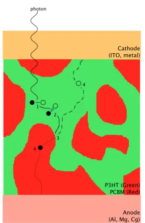
P3HT (Green) PCBM (Red) Cathode (ITO, metal)

Anode (Al, Mg, Cg)

photon

3 4

2

4

1

Figure 1.2. A photon creates a bound

ex-citon in an electron donning material. Dif-fusion causes the exciton to collide with an interface where separation is energetically fa-vorable. The split charge carries are trans-ported to the anode and cathode via an in-ternal potential field. The island to the right will not allow for charge collection. The physics are further explained in [141]. as a photonic crystal that perfectly reflects

part of the visible spectrum leading to

bril-liantly metallic blue wings as is shown in

figure 1.1[148, 113]. Surface structures

can also lead to desirable dewetting

prop-erties, such as that which occurs on the

lotus leaf, insect eyes, peacock wings, and

many other types of living organisms found

in nature [151]. There are also proposed

techniques for using complex interfacial

structures to trap medicinal particles and

create a slow release for the delivery of

medicine [106].

The practical application that

moti-vates this thesis is that there are a

num-ber of processes that benefit from a high

ratio of surface area to volume, yet also

require the interfaces to be well ordered.

For example, organic solar cells generate

charge carriers when excited electron-hole

material [39]. The lifetime of an exciton, however, is short, so typically the electron

accepting and donating materials are well mixed to create a high surface area to volume

ratio (see figure 1.2). The mixing generates isolated islands of material which trap charge

carriers, as well as complex pathways for charge extraction, which lead to losses by

re-combination. Theoretical modeling [154] has revealed that ordered structures with high

surface area to volume ratios would allow a 50% efficiency gain in energy production (see

figure 1.3).

The importance of complex interfacial structures has been established, but the

chal-lenge of how to control formation of these interfaces remains. For small scale

struc-tures (structure on the order of 30-100nm) the field that has arisen to tackle these

construction problems is called nanolithography. The most heavily employed methods

in these fields involve fabrication via the careful application of an energy beam

com-prised of electrons, photons, or ions. This practice has lead to a number of advances

including electron beam production of graphene [159], and photolithography techniques

for semiconductors leading to smaller and faster and transistors (for example [65]).

Figure 1.3. Ordered phase separation of

the bulk heterojunction leads to enhanced efficiency in organic solar cells [154].

Nanoimprint lithography is also used for

cheap and reproducible production of

diffraction grating patterns; these patterns

can be used to generate photonic

crys-tals with enhanced adsorption properties

at targeted areas of the spectrum [85].

Fi-nally, in Aryal et al [6] the authors

success-fully produced two dimensional patterns

mimicking the butterfly wings.

An alternative approach toward

inter-face generation is to ask how we can use

naturally occurring interface instabilities to grow and pronounce emerging structures,

either use the old methods of trail and error, or develop new mathematical and numerical

techniques which allow us both to understand and simulate these emerging structures

in a faster and less expensive environment. In the present work, we focus on the

de-velopment of atomistic to continuum linkage algorithms which model the phenomenon

of crystallization of a solid leading to dendritic pattern formation. We present a brief

history and outline of this problem below, as well as outline the following chapters and

structure of this work.

1.2. An outline for dendrite formation upon solidification

Nanoscale patterning of materials at scales of less than 20nm remains a challenging

problem. Standard techniques, such as lithography, rely on electron and photon beams

to shape materials, yet these methods are difficult to employ at the sub 50nm scale. We

consider the possibility of employing natural interface instabilities during solidification

in order to reliably produce desirable structures. Existing continuum methods for

com-plicated materials may break down at these scales, while direct atomistic simulation is

computationally infeasible. The primary objective of the thesis is to develop methods

ca-pable of efficiently resolving the atomistic computations which may eventually be solved

concurrently with continuum scale approaches. In the present work we develop atomistic

algorithms to furnish closures for continuum methods. We develop novel molecular

tech-niques capable of resolving detail only about an interface with non-periodic boundaries

and accelerated by GPUs. The new algorithms provide a method to determine interfacial

dynamics based on local curvature, employing wedge shaped domains. These dynamics

lead to continuum closures which are used to determine necessary physical parameters

that allow for dendritic patterning at the sub 20nm scale.

This work begins with the question as to how a material will solidify upon the

ex-istence of a crystal seed, which has been of interest since the 1800’s, drawing interest

differential equations to describe this process around 1890 [147], given as

∂T ∂t =Dl

∂2_T

∂x2 for x∈Ωl

(1.1)

T =TM for x∈∂Ωl

(1.2)

HereDl is the thermal diffusivity coefficient in the liquid, Ωl is the liquid domain, TM is

the melting temperature of the material, and ∂Ωl is the boundary of the liquid domain

surrounded by a solid phase of the same material. The equations can be generalized to

allow for the diffusion of heat in the solid, as well as for spatially varying heat capacities

and specific heats. Consideration of multiple dimensions leads to effects of curvature on

the interface, and the question of how heat transfer should be treated at the boundary. A

relationship relating the temperature to the curvature of a sharp interface was proposed in

1932 by Paul Kubelka [89]. However the relationship became known as Gibbs-Thomson

relationship, despite the fact that neither Josiah Willard Gibbs nor William Thomson

(Lord Kelvin) derived it [52]. William Thomson did however derive relationships between

curvature and the surface pressure between droplets separating liquid-vapor phases [133],

and the Gibbs-Thomson relationship has been extended to describe the relationship

be-tween melting temperature and curvature, and then again to encompass relationships

between surface solute concentration and curvature (for example [96, 107]).

Chapter 2 will develop the Stefan equations along with methods to solve the resulting

equations, as well as present continuum and thermodynamic arguments for the

Gibbs-Thomson closure. We will focus on the Gibbs-Gibbs-Thomson relationship as a correction to

equation 1.2 which we will reveal as a linear expansion about curvature and the velocity

of the front. We also briefly review phase-field theory. Where the Stefan problem may

be thought of as a sharp interface model, phase field theory is a diffuse interface model

requiring mesoscale approximations. The two methods are required to be equivalent

in the sharp interface asymptotic limit, and we include discussion of both for the sake

the linear terms in Gibbs-Thompson relationship will be shown to have physical

sig-nificance under certain quasi-equilibrium, thermodynamic assumptions and we will also

revisit improvements made by Herring [58] for the physical descriptions of the curvature

coefficients.

The main difficulty in computational modeling of solidification is the necessity to close

the continuum models. Molecular techniques require far to much detail to be feasible for

direct computation, but the closure laws must reflect the molecular detail. In chapter 3,

we review current methods used to fit Gibbs-Thomson coefficients. The existing methods

all measure the Gibbs-Thomson relationship indirectly and there is evidence that the

relationship will break down for complicated molecular materials. We thus begin to

build a new approach to find this relationship in chapter 4 where we present non-periodic

strategies for molecular dynamics. Such non-periodic strategies may be used in arbitrary

domain shapes, allowing us to directly capture curvature effects on the molecular level

without resolving the entire bulk. Chapter 5 uses these new molecular techniques to

estimate Gibbs-Thomson coefficients for different materials and compares this with the

existing methods presented in chapter 3. The results are used in the continuum theory to

predict the variety in structure from solidifying seeds given the Stefan continuum model

along with the algorithms used to solve these equations from chapter 2. Finally we discuss

the implications and contributions of the work in chapter 6, along with promising future

CHAPTER 2

EXISTING CONTINUUM SOLIDIFICATION MODELS

Interface formation during solidification occurs at scales which render molecular

de-scriptions computationally intractable. At the continuum level, there are two physical

descriptions for solidification processes, and numerical algorithms have been developed

for each. The first method supposes that the phase change may be modeled as a sharp

interface in which the boundary width separating the phases is of infinitesimal width.

The second is classified under phase field models in which the interface is modeled as a

diffuse region of small, but finite thickness. This chapter is dedicated to reviewing these

continuum methods. We start with a discussion on the sharp interface methods, and

next describe the phase field models. We then discuss the underlying assumptions and

limitations of these models. In the discussion on the sharp interface methods, we expose

and derivate the Gibbs-Thomson closure; this closure is used to set the temperature at

sharp interfaces, and is as a constraining equation for asymptotic limits of thin interfaces

in phase field models.

2.1. Sharp interface models

The hypothesis behind sharp interface models is that an interface between liquid

and solid regions may be assumed to have negligible thickness. The interface separates

physical domains, each with prescribed bulk dynamics, and the bulk phases communicate

through closure laws on the interface. The bulk properties determine the dynamics of

the interface, and the properties of the interface determine boundary conditions on the

bulk dynamics. In the present work, we consider solidification of a solid seed in a liquid.

The classical Stefan equations are derived when we assume that temperature is the only

important field variable and that in each region temperature will evolve according to

the heat equation. Allowing the liquid and solid regions to be denoted by Dl and Ds

respectively, temperature evolves within each domain according to

(2.1) ci

∂T

∂t =∇ ·(ki∇T),

fori∈ {l, s}, and whereciis the volumetric heat capacity andkiis the thermal diffusivity.

The jump condition at the interface, called the Stefan condition, is given as

(2.2) LV =−

kl

∂Tl

∂n −ks ∂Ts

∂n

,

whereLis the latent heat of solidification, the subscripts s, l refer to the liquid and solid

regions respectively, and n refers to the normal vector at the interface that points into the liquid region. Finally, V is the velocity of the interface in the direction of n. The Stefan condition equates the energy flux released by the phase transition of the moving

front, with the energy flux due to the transfer of heat, giving local conservation of energy.

Temperature boundary conditions are, as of yet, unprescribed at the interface of

the phase transition. Initially [147], Dirichlet boundary condition were used to set the

melting temperature at the interface to be the melting temperature of the bulk solid,

given as TM. There is, however, a change in free energy due to the presence of an

interface which causes a shift in the melting temperature. This may be closed by the

Gibbs-Thomson relationship, which may be written as

(2.3) T(x, t) =−Cκ−VV +TM,

where κ is the curvature of the solid-liquid interface and is positive when the center of

curvature lies in the direction of the solid, andV is the velocity of the front as described

above. The’s are considered to be constant material properties of the system in question.

Throughout this thesis, we will refer to C as the curvature closure coefficient and V as

positive curvature due to the fact the interface lattice sites have a higher probability

of interacting with liquid particles on the boundary while at the same time having less

average solid particles setting up the lattice potential wells to keep them in the solid

phase. The velocity of the front may also be expressed as a function of under cooling,

where higher undercooling lead to faster rates of solidification; thus, the correction due

to the velocity term arises. In general, each correction term may be anisotrpic and

depending on the orientation of the underlying solid structure. The derivation of this

closure arises from a linearized expansion after solving for the free energy change due to

the presence of a surface and will be explained in detail in the proceeding subsection.

The classical Stefan problem may be compared to the more modern formulation of the

Stefan problem which considers advection in the liquid due to changes in density between

the phases, and may also include advective transport of a solvent which forms the solid

seed in a solute (see, for example, [130]).

2.1.1. The Gibbs-Thomson relationship. Before we begin the derivation of the Thomson equation from equation 2.3, we note that generally speaking a

Gibbs-Thomson equation refers to any equation which relates thermodynamic, geometric, and

system dynamics to the properties of an interface. In addition to the temperature

correc-tion above, other Gibbs-Thomson relacorrec-tionships derive equacorrec-tions for pressure or densities

across an interface [12], the chemical potential across an interface [71], or surface

con-centrations [107]. In all of these relationships derivations are nearly always based upon

an assumption of quasi-equilibrium states that depend on interfacial size, shape,

tem-perature, surface tension, temperature and pressure. A few results are derived from

statistical physics [12], however no such derivation exists for the relationship on melting

temperature. In addition to the quasi-equilibrium theory, non-equilibrium theories have

been developed to account for corrections due to advancing interfaces. This correction,

corresponding to V, is often referred to as a kinetic correction, however we will call this

used to derive the Gibbs-Thomson relationship due to curvature corrections, and next

review the theory for the kinetic correction.

2.1.1.1. Curvature based correction on the melting temperature. A simple derivation of the curvature based correction on Gibbs-Thomson relationship (following [36]) may be

derived starting from the spherical Young-Laplace relationship

(2.4) Ps−Pl =

2γ r ,

where Pi is the pressure in the solid region (s) and liquid region (l), γ is the surface

tension (more accurately, the surface free energy), and r is the radius of curvature of a

spherical seed.

Next we consider the Gibbs-Duhem equation [26] arising from the basic

thermody-namic postulates that (i) we can express the energy U of a system as a function of the

extensive system properties entropy, volume, and particles (S, V, N, respectively), and

that (ii) the relationship is given as U(S, V, N) = T S−P V +µN. Here T is

tempera-ture, P is pressure and µ is the chemical potential. Linearizing the energy about small

perturbations then impliesdU =T dS−P dV +µdN which, in turn, implies that

(2.5) 0 =SdT −V dP +N dµ.

The Gibbs-Duhem relationship can be used to write

ssdT −ρ−s1dPs+dµs = 0,

(2.6)

sldT −ρ−l 1dPl+dµl = 0,

(2.7)

for the solid and liquid phases, where si is the entropy per particle given as Si/Ni, and

ρi = Ni/Vi is the density. We next assume that the external pressure of the liquid is

constant throughout the liquid phase so that dPl = 0. The differentials of the chemical

potentials in the bulk materials are assumed to be equal so thatdµs =dµl [71, 66]. This

may be seen by noting that the Gibbs free energy must be equivalent for each phase at

to be equal in each phase so that µsN = µlN. Subtracting the first equation from the

second gives

(sl−ss)dT +ρ−s1dPs = 0,

(2.8)

L Tm

dT +ρ−_s1dPs = 0,

(2.9)

where the latent heat of the phase transformation is given as L = (sl−ss)T, since this

is the free energy change due to the change in entropy between phases. Taking the

differential of the Young-Laplace relationship in equation 2.4 yields

(2.10) dPs−dPl=d

2γ r

,

Again using the assumption that dPl= 0, we can substitute to obtain

L

TdT +ρ

−1

s dPs = 0,

L

TdT +ρ

−1 s (d

2γ

r ) = 0,

Z

L

TdT = −

Z

ρ−_s1(d2γ r ), Llog T Tm

= −ρ−_s12γ r . (2.11)

Assuming that the corrected temperature is close to the melting temperature, we can

linearize the above equation to find

(2.12) T =Tm

1− 2γ

ρsL

1 r

,

which provides us with the curvature based correction of the Gibbs-Thomson relationship

For general surfaces, the Young-Laplace equation is

(2.13) Ps−Pl=γ

where κ1 and κ2 are the two principal curvatures. This formulation leads to a more

general Gibbs-Thomson closure [5]

(2.14) L T Tm −1 +∆cP T log T Tm

+Tm−T

+vsγ(κ1+κ2)+γa+k1(κ1−κ2) = ∆v(Pl−Patm),

where ∆cP is the jump in specific heat with constant pressure across the phase transition,

Patm is the pressure at infinity and Pl is now the pressure of the liquid at the surface;

vs = ρ−s1 is , a = A/ms is the ratio of the surface area of the phase transition to the

mass of the solid,k1 is called the coefficient of curvature (a correction term to the energy

based on curvature) and ∆v = ρ−1

s −ρ

−1

l is the jump in inverse density related to the

phase transition.

The corrected Young-Laplace condition causes additional terms to rise in deriving the

Gibbs-Thomson relationship, and a corrected scaling law arises. Assuming ∆cP = 0, we

get

(2.15) Ti =Tm−

Tm

L (vsγ(κ1 +κ2) +γa+k1(κ1+κ2)−∆v[Pl−Patm]),

and then assumingκ1 =κ2 and Pl=Patm

Ti = Tm−

2Tmγ

ρsLr

− Tmγa

L

= Tm−

2Tmγ

ρsLr

− Tmγ4πr

2

Lms

= Tm−

2Tmγ

ρsLr

− Tmγ4πr

2

L(4πr3_/3)ρ s

= Tm−

5Tmγ

ρsLr

.

The form of the equation is the same as the simplified relationship, however there is a

corrected scaling factor on the interfacial temperature.

In [58], Herring determined that for droplets surrounded by vapor, the difference in

expressed as

(2.16) µsi −µv =

1 ρs

γ+ ∂

2_γ ∂θ2 1 1 R1 +

γ+∂

2_γ ∂θ2 2 1 R2 ,

whereR1andR2 are the principal radii of curvature in the principal planesP1andP2 (i.e.

orthogonal planes each containing the normal vector at the interface). The θ variables

follow the path of the interface, and thus the double derivatives represent the concavity

of the surface tension γ as the position on the interface is perturbed. The chemical

potential of the solid at the interface is denoted byµsi, and the chemical potential of the

bulk vapor is µv.

The primary mechanism behind Herring’s correction, is to notice that when the

sur-face tension depends on orientation and is twice differentiable, the free energy variation

inherits a second derivative in the leading order term. We compute the change in free

energy caused by a variation in the surface via a functional derivative on the interface.

We begin by rederiving the right-hand side of the Young-Laplace equation for a single

dimension, and first assume a constant γ with respect to orientation. The interfacial

energy may be given as Fsr = R

γds, where we integrate over the surface. Letting θ

be the tangent angle to the surface, assume it is small so that θ ≈ dy/da, where y

is the height of the surface and a parametrizes the arc length A. We then have that

ds = sec(θ)dφ ≈ (1 + (dy/da)2/2)da. Taking a small variation over the interface

de-scribed byy(a) gives

δFsr ≈ Z A

0

1 + 1 2

d(y+δy) da

2!

γ− 1 + 1 2 dy da 2! γda = γ Z A 0 dδy da dy

dada+O(δy

2₎

= −γ

Z A

0

δyd

2_y

da2da

= −γ

R

Z A

0

δyda

= −γ

where the third line comes from integration by parts, the fourth comes using the

relation-ship that curvature is the inverse of the radius is the second derivative ofywith respect to

a, and the fifth line equates the change in volume due to the change in surface. Assuming

we are at equilibrium and that the variation maintains the energy, the Young-Laplace

equation arises when we assume that the pressure redistributes to balance this change,

giving

(2.17) (Ps−Pl)δv+δFsr= 0.

The additional factor of two arises from the transition from two to three dimensions. We

can next ask how the free energy differential changes when we allow γ to depend on θ.

Carrying out similar analysis to the above and Taylor expanding about θ = 0 (without

loss of generality) gives

δFsr ≈ Z A

0

1 + 1 2

d(y+δy) da

2!

γ(d(y+δy)

da )− 1 + 1 2 dy da 2! γ(d(y da )da

δFsr ≈ Z A

0

1 + 1 2

d(y+δy) da

2!

γ(0) +γ0(0)d(y+δy) da +γ

00

(0)

d(y+δy) da

2!

...

...− 1 + 1 2

dy da

2!

γ(0) +γ0(0)dy da +γ

00 (0) dy da 2! da = Z A 0 dδy da dy

daγ(0) + dδy

da dy daγ

00

(0) +O(δy2)da

= −γ(0) +γ 00₍₀₎

R δv,

which gives the Herring correction to the surface tension. In three dimensions, the Herring

correction yields a new Gibbs-Thomson equation for temperature given as

(2.18) Ti =Tm 1−

1 ρL

X

i=1,2

(γ+∂

2_γ ∂θ2 i ) 1 Ri ! ,

The Gibbs-Thomson closure has been corrected over the past century and a half,

however there is still controversy as to what correction terms are necessary for an

by positing functions for the surface tension as a function of orientation. The idea

be-hind this assumption is that the interfaces of interest in solidification are typically 1000

times larger than the interface width (roughly O(µm) : O(nm)) and thus the surface

is considered locally flat. It is interesting to note that the curvature effects the

Gibbs-Thomson relationship attempts to capture, assumes that the surface tension will not

depend on curvature. In fact, there are known surface tension corrections for curvature

(see for example [66]), yet there is no existing solidification study that takes this effect

into account.

The temperature correction methods rely on linear expansion methods to solve for

temperature corrections. For multicomponent systems such as metal alloys, however,

there has been a great deal of work that has demonstrated the importance of adding

non-linear effects and corrected models for Gibbs-Thomson relationships between interfacial

concentrations and curvatures [107, 120]. In these works, the authors show that the

classical assumptions fail and develop novel equations that seek to correct the earlier

models, however they do not attempt to determine corrected melting temperatures.

In addition to the equilibrium closure, a kinetic coefficient has also been added to the

Gibbs-Thomson relationship to adjust for non-equilibrium effects. We shall review this

correction presently.

2.1.1.2. Velocity corrections to the Gibbs-Thomson relationship. We next address the velocity term of equation 2.3. In addition to the curvature based corrections of the

inter-facial temperature, non-equilibrium effects also play an important roll for solidification.

The idea behind the corrected temperature-velocity relationship comes form studies on

interface dynamics [69] which relate the temperature of a front with the speed at which

it solidifies.

Current theory behind evolving interfaces describes the rate of the advancing front

as a balance between particles from the liquid becoming a part of the solid phase with

simple relationship

(2.19) V =V+−V−,

where V is the velocity of the interface, V+ _{is the rate of advancement and V}− _{is the}

rate of retreat. The velocity terms are refined by setting

(2.20) Vi =af νi,

where a is the change in the local length of the front due to an attachment or

detach-ment event, f is the fraction of the surface area with sites available for attachment or

detachment, and nui _{is the rate of attachment/detachment. The first two factors are}

chosen based on the orientation of the solid, where the third is unknown and based on

out-of-equilibrium dynamics. The constant of proportionality between νs and νl is

as-sumed to be given by a Poisson process which is governed by the underlying particle

energy difference in the liquid and solid states. This leads to rate constants which are

proportionally closed via a Boltzmann distribution based on the jump in potential energy

for each particle. In a bulk thermodynamic point of view, νi _{can also be thought of as}

jump in the energy associated with being in each phase.

We must then determine the change in the Gibbs-free energy across the phases. For

each phase, the Gibbs free energy and its variation is given as

Gi = µiNi,

∆Gi = µidNi,

for i ∈ {l, s} for liquid and solid. At the equilibrium point the two energies must be

equival in order for both phases to exist stably. Due to the motion of the interface, we

expand about the differential of each phase to get

∆Gi = µinterfacei dNi

≈ dNi(µbulki +

∂µbulk_i ∂T

P

∆T +

∂µbulk_i ∂P

T

∆P)

= dNi(µbulki +

∂2_H i

∂T ∂Ni

P

∆T +

∂2_H i

∂P ∂Ni

T

∆P)

= dNi(µbulki − ∂Si ∂Ni P ∆T + ∂Vi ∂Ni T ∆P),

whereH is the enthalpy. To find the change in the Gibbs free energy associated with the

interface, we then integrate

Z

d(Gl−Gs) = − Z

∂Sl

∂Nl

P

∆T dNl+

Z

∂Ss

∂Ns

P

∆T dNs,

(2.21) + Z ∂Vl ∂Nl T

∆P dNl−

Z

∂Vs

∂Ns

T

∆P dNs,

∆G=Gl−Gs = −(Sl−Ss)∆T + (Vl−Vs)∆P,

(2.22)

= −L∆T /Tm+ (Vl−Vs)∆P

(2.23)

where we have again used the fact that µbulk_s = µbulk_l . Since we presently assume a flat

interface, the pressure correction is absent so that the energy difference in moving across

the interface is given as−L∆T /Tm, with ∆T =Ti−Tm. Thus for an undercooled surface,

it is energetically favorable for particles to attach to the solid phase.

With the above arguments, we may determine the constant of proportionality between

attachment and detachment events to write

(2.24) ν−=ν+exp

−∆G

kT

=ν+exp

−L∆T

kTmT

.

We can then write the velocity of the front as

(2.25) V =af ν+

1−exp

−L∆T

kTmT

and linearize about small interfacial temperature fluctuations to get

(2.26) V ≈af ν+ L∆T

kTmT

.

Given the temperature correction, we can find the velocity, and subsequently

(2.27) Ti ≈Tm(1−

kTm

af Lν+V).

There are other closures for this correction as well. In [157], Wilson proposes that an

activation energy associated with atom mobility to account for the probability of leaving

or entering the solid interface. The activation energy was fit based on the model, and

the model was shown to fit well for the crystallization of silicon [69].

Molecules with pair interactions prescribed by the Lennard-Jones potential, fail for

the model proposed in [157]. These ensembles may, however, be accurately modeled by

allowing the the velocity V to scale with √T in [20, 21] the new model given as

(2.28) V = a

λ

r

3kT m f

1−exp

−∆G

kT

,

where λ is a constitutive correction term and physically interpreted as the distance an

atom must move to join the crystal. In this case we have a nonlinear correction to the

temperature. Setting T =Ti, linearizing the above exponential function, and solving the

resulting equation for the interfacial temperature gives

(2.29) Ti =Tm

1 + kTmλ

2

6a2_f2_L2V

2₋p

kmT3 mV λ

p

12a2_f2_L2_+kmT mV2λ2

1 6a2_f2_L2

.

We can linearize about the square root term and discard the terms of O(V2_{) and above}

to get

(2.30) Ti =Tm 1−

r

kT3

mm

3 λ af LV

!

which leads to a different physical interpretation of the velocity closure coefficient in the

In addition to the difficulty associated with choosing the proper model based on

molecular potentials, there have been no molecular or kinetic Monte Carlo verifications

to account for the effect of curvature on the velocity closure coefficient. To our knowledge,

there is no theory tying the curvature of an interface with the speed of the advancing

front. Such a proposal however is easy to posit. In equation 2.22 the interior pressure

differential may be replaced with the Young-Laplace equation. Futhermore, we can admit

the possibility that ν+ depends on the interfacial temperature as is predicted in the

Lennard-Jones fit from [20] and equation 2.28 which gives

(2.31) V = a

λ

r

3kT m f

1−exp

−L(Ti−Tm)

kTmT

− 2γ

krρsT

,

Similar analysis leads to a corrected equation

(2.32) Ti =Tm 1−

2γ Lρs 1 r − s 3kmT3

m(rρs−2γ/L)

rρs

λ 3af LV

!

,

providing a relationship on how the velocity closure coefficient will depend on curvature.

Note that the classical Gibbs-Thomson correction arises naturally in the second term of

the right hand side. Furthermore, this equation reduces to the flat interface result of

equation 2.30 in the limit r → ∞. A similar correction may be made with the Herring

contribution. Note however that the assumptions from the linearization require that the

perturbed interfacial temperature are small, and thus _Lρ2γ

s

1

r 1, thus we can approximate

this equation as

(2.33) Ti =Tm

1− 2γ

Lρs 1 r − p 3kmT3 m λ 3af LV

,

to recover the full Gibbs-Thomson equation, corrected both for the curvature and velocity

closure effects.

2.1.2. Algorithms for sharp interface methods. With the physics of the sharp interface problem having been reviewed, we now review algorithms that are used to

tracking methods, and we review these below. Other methods exist such as boundary

integral methods, finite element adapting meshes for enthalpy formulations, and others,

but we omit discussing them in the present work.

2.1.2.1. Level set methods. Utilizing the assumption that there is a sharp interface be-tween the liquid and solid regions, level set methods embed this interface via a discretized

field variable which is tracked on a cartesian mesh. The interface is embedded by having

the field variable hold values based on how far the surface is away from the interface.

The zero level set of this field represents the desired interface, and hence the description

‘level set methods.’ The apparent disadvantage of this method is that we are increasing

the dimensionality of the surface and requiring an additional amount of memory

stor-age. The advantage is that by advancing the field, as opposed to the surface, we avoid

difficulties in tracking the surface directly; because of this, moving from two to three

dimensions results in no additional algorithmic complexities

For solidification, both finite difference and finite volume level set methods have been

employed. In the present section we will focus on the conceptually simpler finite difference

schemes. We will outline ideas from [31] and [50].

The basic idea of the algorithm is to use operator splitting by first solving the heat

equation for a fixed interface and then evolving the interface with a fixed temperature

field. This is accomplished by discretizing the domain on the standard regular cartesian

grid, in which we embed the interface on a field described at these points. The field takes

on values by having the regular grid points hold the minimum distance from the interface.

To extract the interface, we can interpolate nodes of the interface that lie between grid

points where there is a change in sign. More sophisticated interpolation schemes will

lead to higher accuracy in recapturing the interface, however linear schemes are often

sufficient and also widely employed in practice.

With the phase of the material assigned by the sign of the embedded field, we can now

expose the techniques used to solve the heat equation. In considering grid points which

scheme for the heat equations (equation 5.11). For example, taking a backward Euler

approach and assuming that the thermal diffusivity is constant throughout the region

will yield

(2.34) T

n+1

i −Tin

∆t =

k c

T_i+1n+1−2T_in+1+T_in+1₋₁

∆x2 ,

where T_in is the temperature at node point i at time step n, ∆t is the size of a time

step, ∆x is the length of the spatial discretization, and c and k are the volumetric heat

capacity and thermal diffusivity as given above in equation 5.11.

This is not valid when the interface cuts between two finite difference node points.

To circumvent this issue, suppose that the interface cuts between xi and xi+1. The

Gibbs-Thomson relationship specifies the temperature at the interface and thus we have

Dirichlet boundary conditions. Before we can solve the heat equation about grid point

i, we first need to find the interfacial temperature at the interfacial position between xi

and xi+1. This temperature will be a function of the interfacial velocity VI according

to the Gibbs-Thomson relationship; the Stefan condition may be used to determine the

interfacial velocity, however it requires knowledge of the interfacial temperature. We thus

have a two dimensional system with two unknowns

VI =

1 L

−kj

∂T ∂~n

, (2.35)

TI =Tm−CκI −VVI,

(2.36)

whereTI is now defined as the interfacial temperature, andκIis the interfacial curvature.

We then discretize these equations to get

VI =

1 L

−ks

TI−Tis √

2dx

−kl

TI −Til √

2dx

,

TI =Tm−CκI−VVI,

whereTis andTil are the temperatures a distance of √

2dx away from the interface in the

values are found by interpolating from the known mesh via the equation

Tik =(1−fx)(1−fy)T(i+1)j+ (1−fx)fyT(i+1)(j+1)+fx(1−fy)T(i+2)j+fxfyT(i+2)(j+1).

(2.37)

Here we have assumed the four points surrounding the location a distance √2dx in the

normal direction are of a single phase. We next find the curvature at points xi and xi+1

by using the fact that the curvatureκl can be related to the gradient of the normal vector

(2.38) κ=∇ ·n=∇ · ∇φ

|∇φ| =

φ2

yφxx−2φxφyφxy +φ2xφyy

(φ2

x+φ2y)3/2

,

where φ is the field that embeds the level set. Taking typical finite difference schemes,

we can determine the curvature each point on the mesh and then interpolate it to the

interface, similarly to equation 2.37.

We can then write a stencil for the heat equation depending on the interpolation

schemes that we choose. Taking a linear interpolation to the interface yields

(2.39) T

n+1

i −Tin

∆t =

k c∆x

TI−Tin+1

xI−xi

− T

n+1

i −T

n+1 i−1

∆x

.

This closes the description of the heat equation. After this step is complete we next

evolve the interface. To evolve the interface, we first determine the different energies

entering and leaving the system via equation 2.2. This is done in the standard way,

interpolating to the boundary as was done above. Knowing the velocity at the front we

then extend the velocity to the entire fieldφ, denoting this velocity field asF. To extend

the velocity field there are several proposed methods. The original method used in [31]

relies on continuously extending the jump of the derivatives away from the front. To

accomplish this, we may set

u1_t + sgn(φφx)u1x = 0,

with u1 _{= [∂T /∂x] and u}2 _{= [∂T /∂y], sgn is the sign function, and τ is a fictitious}

time parameter that will be used to determine the extended velocity field. The idea is

to advect the contributions of the velocity at the interface throughout the domain from

each point of the interface. The velocity, which will be normal to the level set at any

value of φ, is then taken to be the norm of these advected velocities. The issue with this

method is that the field φ does not maintain itself as a distance function away from the

level set which can lead to errors in the interface and present problems with numerical

stability. The solution is then to reset the field as the signed distance function. In [31]

an iterative process is used to relax the field back toward the signed distance function.

Instead of advecting the field via the above method, we can use the Fast Marching

Method [1] which extends the front velocity to the field in a way that preserves the

distance function. The idea is similar to the one above, in that it also advects the field

away from the known values on the mesh, however instead of summing over a variety of

solutions, it advects a unified wave front from the surface and checks the validity of each

point as it marches along.

With the velocity field now extended, we can advect the level set points numerically

using a simple upwind scheme

(2.40) φn+1_i =φn_i −dt max(0, Fi)∇++ min(0, Fi)∇−

,

where

(2.41)

∇+/− = max(0, D−x/+x) + min(0, D+x/−x) + max(0, D−y/+y) + min(0, D+y/+y),

and D+/−x/y _{is the first order one sided finite difference derivative. From here we can}

apply the diffusive and advective schemes as a split operator.

In summary, the algorithm will work as follows:

(1) InitializeT(~x, t) and the interface Γ. Initialize φ.

(2) Find the temperature at each point of Γ that intersects a line of the mesh.

(4) Find the velocity at each point on Γ.

(5) Extend the velocity on the path to φ, denoting this field F

(6) Advect F

(7) Determine Γ by interpolating the new values ofφ.

(8) Repeat.

Higher order corrections have been constructed and implemented [49, 104], as

com-pared to the low order method described above. Many of the level set methods are also

also unable to globally conserve energy about the boundary, however due to continually

improved methods, current methods are able to conserve energy energy upon numerical

discretization [130].

As mentioned above, a minor downside to implementing level set solidification

al-gorithms is that they require extra memory to store φ. There also is the requirement

of constantly moving back and forth between the interfacial and field descriptions to

track where the phase transition occurs. These produce minor algorithmic complexities

however, and the solutions found by these methods are qualitatively accurate and agree

well with solvability theory, an analytic theory that predicts ranges for the tip velocity

[83]. Furthermore, they allow for low resolution about the interface, compared to the

phase field methods that have a sharply changing phase field about the interface, and

thus require high resolution. As a final advantage, level set methods have proven to be

relatively easy to implement in both two and three dimensional settings.

2.1.2.2. Interface tracking methods. Interface tracking methods for solidification are sim-ilar to the level set methods, as both assume a sharp interface between the solid and

liquid phases. Algorithmically however, the interface is directly tracked and advected

throughout the simulation, rather than being embedded in an extended field. Interface

tracking methods applied to solidification appeared before similar application of level

set methods, a notable one appearing in 1996 by Juric and Tryaggvason [72] (3 years

before the first level set methods were used). These methods have since been

has waned, most likely due to algorithmic complexities in generating and updating the

moving Lagrangian interface.

These methods suffer from the same problem of non-globally conserved energy,

how-ever no such method has come along to fix this problem as has been accomplished in level

sets [130]. While the algorithms are diverse in nature, they can be thought of precisely

as the above level set description, in which the interface is advanced directly instead

of being embedded within the level set. While there are algorithmic variations among

both level set and interface tracking methods, the above pseudo code for the level sets

demonstrates a potential interface tracking methods algorithm: operator splitting may

again used and the heat equation is solved identically as in the level set method. The

exception is that the interfacial discretization is redefined at each time step instead of

being embedded in the field variable φ.

The method may be seen as having an advantage over the level set methods in that it

no longer requires interpolating the path at the grid line intersections and it avoids moving

between embedded and explicit representations of the interface. Difficulty is preserved

however, when we acknowledge that the discretization of the path must adapt with the

changing front. Growing fronts will require insertion of node points and methods are

developed to determine how to place them. Additionally, node points may cross, leading

to loops in the path and the necessity to remove points no longer on the interface. Case

based algorithms are fully capable of handling these nuances at the interface, but care

must be taken in accounting for all possibilities.

2.1.3. Assumptions and limitations. The main limitation of the continuum sharp interface model is that we do not know, a priori, the interfacial dynamics employed in the Gibbs-Thomson closure. As discussed above, there has been a great deal of effort to

properly close this equation and relate it to the microscopic properties of the materials.

At the molecular scale, methods have been developed to determine the resulting physical

constants necessary to close the Gibbs-Thomson relationship, and these will be discussed

field models have lead to several distinct possibilities for a Gibbs-Thomson closure,

how-ever there are minor inconsistencies in the results. We will continue this section by review

phase field models.

2.2. Phase field models

Phase field models treat the interface as diffuse across some width w. If taking on a

physically meaningful model, this width should be proportional to the capillary length

between the changing phases, however in many physical scenarios, dendritic fingering

structures occur at length scales on the order of microns, while molecular dynamics

suggest that the capillary length scale is roughly three orders of magnitude smaller.

This length scale disparity makes phase field computation difficult, and in many cases

intractable. Never-the-less supposing larger values for the interface widthwhas provided

a useful tool in modeling problems involving solidification as will be discussed below.

The main advantage of phase field models for computation is that they mitigate

nu-merical noise, grid anisotropies, and other issues that occur in sharp interface modeling

by replacing the challenge of reconstructing advancing fronts with the challenge of

cre-ating grids capable of resolving the diffuse interface. Similar to level set methods, a new

field variableφ is added to the equations which is set to be 1 in the solid phase, 0 in the

liquid phase, and smoothly varies between phases across the front. The evolution ofφ is

found by proposing an evolution equation to minimize a proposed free energy functional,

given in the form of

(2.42) F =

Z

V

dV

w2

2 |∇φ|

2

+f(φ, T, ...)

,

wheref is the free-energy density that depends on the phase field variableφ, temperature,

and possibly other important field variables such as the concentration of a solute. In this

equationf is typically taken to be a low order polynomial inφwith coefficients depending

on physical constraints, with the gradient of φ included as a truncated expansion of the

surface effects on the free energy [91]. Linear effects from the polynomial are omitted

due to the observation that the free energy should be rotationally symmetric.

Phase field models begin as phenomenological expansions of the local free energy.

From the phenomenological descriptions, polynomial coefficients are fit from

thermody-namic arguments to make the free energy descriptions consistent with known theory.

Indeed, the development of phase field models are looked and constructed at in one of

two ways: the first is a construction based on thermodynamic arguments; the second is

purely as a mathematical descriptor which is used to represent a diffuse interface [13].

Once a free energy description is chosen, we must propose an evolution equation

that tracks the systems heat exchange, we may take a similar equation as the diffusion

equations above, however we must include the latent heat exchange as a source term,

as there is no definitive boundary condition any more. Such an equation tracking heat

exchange is now written as

(2.43) cp

∂T ∂t +L

∂φ

∂t =∇ ·(k∇T),

wherecp is the heat capacity,kis the specific heat,Lis the latent heat, andT is again the

temperature. In the sharp interface model the latent heat production was accounted for

directly by equating the energy production of the propagating front with the energy flux

from the boundary, however here latent heat is introduced to the system at the interface

as φ changes from one phase to another (represented in the second term). The heat

capacities and specific heats are known in the bulk phases, however simple constitutive

relationships can be used to link the domains. The simplest and most often used closure

is to let cp = φcs + (1− φ)cl where the subscripts {l, s} refer to the liquid and solid

regions respectively; a similar equation may be used to find the specific heat across the

phase transition.

In addition to resolving the heat exchange, we must also minimize the free energy.

To do this we want to find the interfacial energy found by the changingφ and allow φto

functional derivative must then be zero at equilibrium

(2.44) δF

δφ = ∂f ∂φ −w

2_∇2

φ= 0.

In order to relax the system to the equilibrium state, constitutive models can be used to

describe the relaxation process. In solidification, the most commonly used is called the

model A equation, which accounts for simple exponential relaxation. It is written as

(2.45) τ∂φ

∂t =−

∂f ∂φ −w

2_∇2_φ

,

whereτ is a characteristic time scale of relaxation. More complicated models exist which

seek to conserve various physical quantities (see [59]).

In minimizingF, there is a competition between the gradient ofφand the polynomial

f (see equation 2.42). We note that the free energy of a pure phase (given by the

polynomial f in equation 2.42) must be at a local minimum when φ is either 0 or 1 (in

the liquid or solid phase) since we would otherwise not have a separation of phase, and

thus this term will be minimal when the interface is infinitely thin. The integral of the

squared gradient term, however, is minimized as the interface becomes infinitely large.

This competition between free energy contributions sets the width of the interface.

2.2.1. Algorithms for phase field methods. As we noted before, there is a roughly three order of magnitude difference between the interface width and the radius of

curva-ture associated with dendritic tips. This leads to a large discrepancy of scales which cause

the resulting physical equations in the previous section to be quite stiff. To overcome this

issue, there have been a series of adaptive meshing algorithms that have sought to sharply

resolve the interface while zooming out to account for heat transport in the surrounding

pure phases [103, 111, 112, 109]. In [112], for example, Provatas, Goldenfeld, and

Dantzig close the phase field model with a free energy described by [78]. The authors

then develop an adaptive finite element quad tree structure that is able to efficiently

cap-ture the evolving interface. Without such a method the authors demonstrate that grid

at low undercooling (leading to slower fronts and sharper interfaces) which is unfeasible

computationally. Their results agree well with known theory for high undercooling, but

do not for low undercooling.

For pure melts, Karma and Rappel [79] reformulated the sharp-interface analysis via

a phase field model to recover the sharp interface model. The artificially thick interface

analysis demonstrates that the Gibbs-Thomson relationship at the solid-liquid interface

can be recovered with w much larger than the microscopic surface tension length. This

analysis also allows for asymptotic limits in which the interface can be assumed to be in

local thermodynamic equilibrium, and thus the velocity closure constant (i.e.

tempera-ture correction via the velocity of the front) can be discarded. This artificially diffuse

interface method has lead to a hybrid sharp interface-diffuse phase-field method which

is able to conserve energy and achieves the theoretical predictions at low undercooling

[130].

2.2.2. Assumptions and limitations. While the phase-field methods have proved remarkably useful, they rely on referencing the macroscopic sharp-interface equations

for proper closures able to capture experimental predictions. Care must be taken in

construction of the phase field closures to ensure that the continuum limits are achieved,

and phase-field models are verified based on their ability to asymptotically achieve the

continuum limit rather than taken as a more fundamental physical closure. Assuming a

Ginzburg-Landau theory, Caginalp was the first to show the possibility for recovering the

Gibbs-Thompson closure from a phase field assumption [23, 24], however the interfacial

width needed to be smaller than the capillary length for the sharp interface limit to

be achieved. Karma and Rappel relaxed this restriction allowing the sharp interface

limit to be achieved with a method that allows for a phase-field interface width which is

larger than the capillary length [78, 79]. Despite these advancements the closures and

parameter estimates of phase-field theory are still dependent on the assumptions of the

A second non-physical consequence of phase-field modeling is that numerics performed

using coarse, finite-difference meshes exhibit side branching typical of real dendrites

be-cause discretization errors introduce noise into the calculation. However, a coarse square

mesh can also induce grid anisotropy. As the computational mesh is refined, side branches

disappear in phase-field models, which is an unphysical consequence of the model. To

avoid this problem noise may be introduced to induce side branching. This is typically

implemented by adding stochastic forcing to the phase-field equations [42, 92]. More

recently, noise has been introduced by Monte Carlo techniques which solve the heat

equation away form the interface, essentially constructing a mesh free method away from

the interface; this method provides the noise necessary for side branching and

addition-ally circumvents the necessity of adaptive meshing [109]. To contrast this feature with

sharp interface models, the continuum model contains no inherent length scale in the

dimensional analysis, and thus the fingering process occurs at all length scales and

in-dependently of the mesh structure. Care must be taken in all methods to avoid grid

anisotropy.

Up to this point, we have reviewed phase-field models that are parametrized by a

single phase-field scalar variable. The assumption is that we can take the solid lattice

and liquid density probability density distributions and reduce this function to a single

order parameter [56, 81]. Multiple-order phase field methods exist as well, which are

able to capture richer dynamics across phases (see for example [13]). Anisotropy is

typically taken into account in an ad hoc manner, as is done in the sharp interface

method. Alternatively, one can keep the multiple-order parameter picture and naturally

derive anisotropic effects [16].

The diffuse, but small interface also requires proper grid resolution in order to

ac-curately compute the free energy. This requires adaptive meshing techniques to resolve

interfaces which provide more thoughtful algorithms for three dimensional structures.

Three dimensional solidification via phase field models has been achieved in a number of

Sharp interface and Phase-field modeling provide tools for analyzing solidification

of many types of materials. The remaining task is how to close parameters for given

materials either through the Gibbs-Thomson relationship or for the parameters for the

free energy formulation of the phase-field equations. Having reviewed the descriptions

of continuum laws at both macroscopic and mesoscopic scales given the Gibbs-Thomson

closure, we turn now to how molecular simulations allow us to obtain coefficients for the