PDE SOLVERS FOR HYBRID CPU-GPU ARCHITECTURES
Michael Malahe
A dissertation submitted to the faculty at the University of North Carolina at Chapel Hill in partial fulfillment of the requirements for the degree of Doctor of Philosophy in the Department of
Mathematics in the College of Arts and Sciences.
Chapel Hill 2016
ABSTRACT
Michael Malahe: PDE Solvers for Hybrid CPU-GPU Architectures (Under the direction of Sorin Mitran)
Many problems of scientific and industrial interest are investigated through numerically solving partial differential equations (PDEs). For some of these problems, the scope of the investigation is limited by the costs of computational resources. A new approach to reducing these costs is the use of coprocessors, such as graphics processing units (GPUs) and Many Integrated Core (MIC) cards, which can execute floating point operations at a higher rate than a central processing unit (CPU) of the same cost. This is achieved through the use of a large number of processors in a single device, each with very limited dedicated memory per thread. Codes for a number of continuum methods, such as boundary element methods (BEM), finite element methods (FEM) and finite difference methods (FDM) have already been implemented on coprocessor architectures. These methods were designed before the adoption of coprocessor architectures, so implementing them efficiently with reduced thread-level memory can be challenging. There are other methods that do operate efficiently with limited thread-level memory, such as Monte Carlo methods (MCM) and lattice Boltzmann methods (LBM) for kinetic formulations of PDEs, but they are not competitive on CPUs and generally have poorer convergence than the continuum methods.
ACKNOWLEDGEMENTS
This work would not have been possible without the support of my advisor, Sorin Mitran. I am thankful for his dedicated mentoring, not just in my PhD work, but also in planning for the career beyond. His guidance has been invaluable.
I am grateful to the members of my PhD committee, Jingfang Huang, Boyce Griffith, Richard McLaughlin and Julia Kimbell, for their advice and input at various stages of the work. I also appreciate the contributions of Cass Miller in this area.
I am grateful to the National Research Foundation of South Africa (NRF) and the United States Department of State for the award of an NRF/Fulbright Scholarship for Doctoral Studies Abroad for the first three years of my work. This work would never have begun without their support. For funding grants that supported the continuation of my work, I would like to thank the National Science Foundation and the National Institutes of Health.
I would also like to thank UNC Research Computing, in particular, Mark Reed, Jenny Williams and Sandeep Sarangi, for sharing their expertise, and for help with the logistics of running large scale computations.
TABLE OF CONTENTS
LIST OF FIGURES . . . ix
LIST OF TABLES . . . xii
LIST OF ABBREVIATIONS . . . xiii
CHAPTER 1: INTRODUCTION . . . 1
1.1 Numerical Approaches to PDEs . . . 1
1.2 Applications . . . 2
1.2.1 Inhomogeneous diffusion . . . 2
1.3 Processor architectures . . . 4
CHAPTER 2: COMPUTER ARCHITECTURES . . . 7
2.1 CPUs . . . 7
2.2 GPUs . . . 7
2.2.1 Memory . . . 7
2.3 MICs and other architectures . . . 9
CHAPTER 3: CONTINUUM METHODS . . . 10
3.1 Finite Difference Methods . . . 10
3.2 Parallelization . . . 11
3.2.1 CPU . . . 11
3.2.2 GPU . . . 11
3.2.3 MIC . . . 12
CHAPTER 4: LINEAR SOLVERS . . . 14
4.1.2 Enriched subspace GMRES . . . 19
4.2 Classical preconditioners . . . 20
4.3 Deflation preconditioned GMRES . . . 24
4.4 Multigrid methods . . . 25
4.4.1 Two-grid multigrid . . . 25
4.4.2 Two-grid convergence . . . 28
4.4.3 Parallel full multigrid . . . 31
4.4.4 Semicoarsening multigrid . . . 31
CHAPTER 5: KINETIC METHODS . . . 33
5.1 Feynman-Kac formulation . . . 33
5.1.1 Sample path integration . . . 34
5.1.2 Adaptive time-stepping . . . 34
5.2 Feynman-Kac formulation for principal eigenpair . . . 36
5.3 Multiple eigenpairs . . . 38
5.3.1 Cascading scheme . . . 38
5.3.2 Dealing with degeneracy . . . 40
5.3.3 Restarted scheme with dynamic branch time choice . . . 41
5.4 Generalization . . . 44
5.5 Implementation . . . 46
5.5.1 Pseudorandom number generator . . . 46
5.5.2 Memory management . . . 48
5.6 Multiscale Random Walks . . . 53
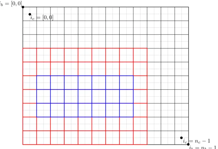
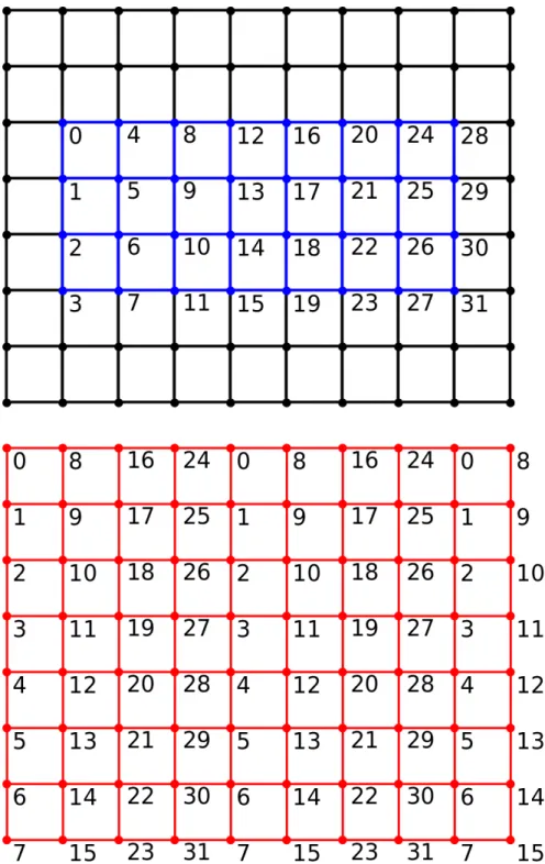
5.6.1 Restriction and prolongation in 2D . . . 53
5.7 Results . . . 55
5.7.1 Decay cutoff times . . . 56
5.7.2 Timestep size . . . 57
5.7.3 Number of samples . . . 57
5.7.4 Filtering . . . 57
CHAPTER 6: CONTINUUM-KINETIC HYBRID METHODS . . . 71
6.1 Concurrent computation . . . 71
6.2 Hybrid enriched GMRES . . . 73
6.2.1 Results in 1D . . . 73
6.3 Hybrid deflated GMRES . . . 73
6.3.1 Implementation in 2D . . . 78
6.4 hybrid deflated GMRES (HDGMRES) results in 2D . . . 80
6.4.1 Effect of eigensolver parameters on convergence . . . 82
6.4.2 Varying diffusivities . . . 85
6.5 HDGMRES parallel efficiency . . . 96
6.5.1 Large memory configuration . . . 96
6.5.2 Small memory configuration . . . 103
6.5.3 Modifications for petascale implementations . . . 103
CHAPTER 7: DISCUSSION AND CONCLUSION . . . 108
7.1 Discussion . . . 108
7.2 Future Directions . . . 109
7.3 Conclusion . . . 109
LIST OF FIGURES
1.1 Example domain for Equation (1.3). Dirichlet conditions in the interior boundaries and Neumann conditions on the outer boundary would be notatedΓD =∂Ω1∪∂Ω2∪∂Ω2,
andΓN =∂Ω0. . . 3
1.2 History of the three dominant processor architectures in terms of peak TFLOP/s throughput with perfect parallelization [1, 2, 3] . . . 6
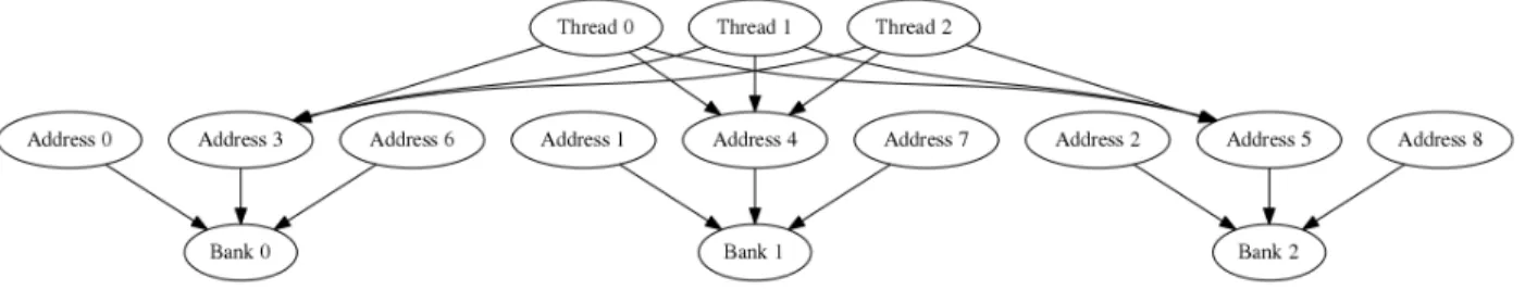
2.1 Threads accessing the same memory location in each bank. These broadcast operations do not incur any serialization. . . 8
2.2 Threads accessing memory from completely separate banks. This is the best case scenario. . . 8
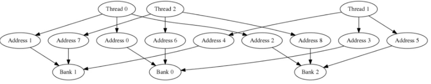
2.3 Threads accessing memory from contiguous memory addresses. This is the worst case scenario. . . 9
5.1 The restarted cascading scheme . . . 43
5.2 The block assignment scheme . . . 49
5.3 The shared memory assignment scheme. Blue: dimensions of the thread block. Red: dimensions of the shared memory. . . 51
5.4 The scheme for reading coefficients from global memory to shared memory . . . 52
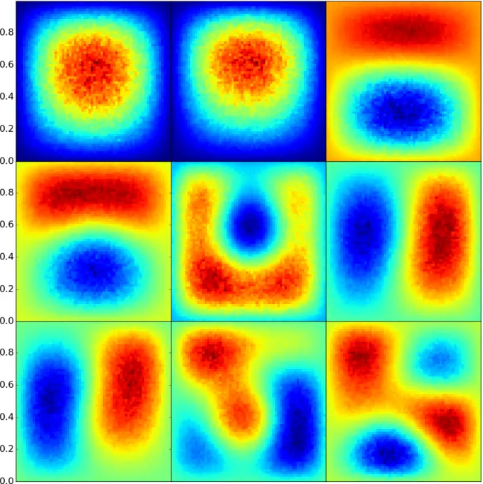
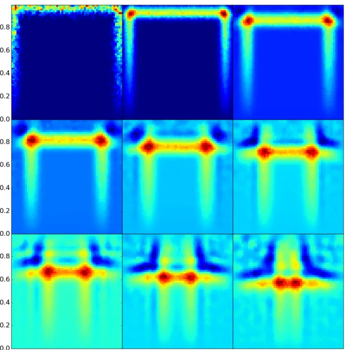
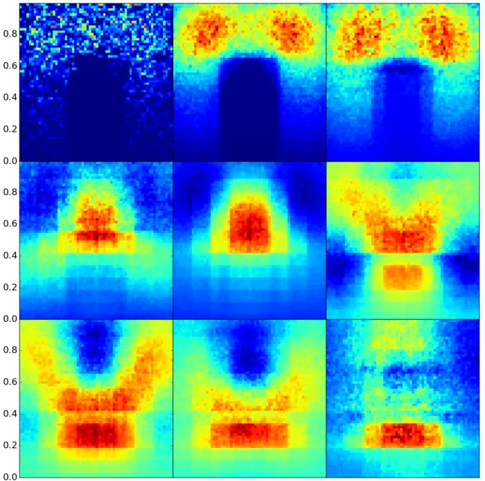
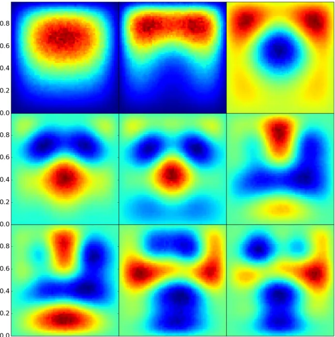
5.5 Eigenvectors from the restarted cascading eigensolver, with decay fraction= 0.01 . 58 5.6 Eigenvectors from the restarted cascading eigensolver, with decay fraction= 0.99 . 59 5.7 Eigenvectors from the restarted cascading eigensolver, with decay fraction= 0.4 . . 60
5.8 Eigenvectors from the restarted cascading eigensolver, with exit probabilityp= 0.5 . 61 5.9 Eigenvectors from the restarted cascading eigensolver, with exit probabilityp= 0.1 . 62 5.10 Eigenvectors from the restarted cascading eigensolver, with exit probability p= 0.0001 63 5.11 Eigenvectors from the restarted cascading eigensolver, with 4 samples . . . 64
5.12 Eigenvectors from the restarted cascading eigensolver, with 16 samples . . . 65
5.13 Eigenvectors from the restarted cascading eigensolver, with 128 samples . . . 66
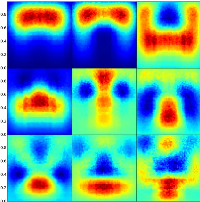
5.14 Eigenvectors from the restarted cascading eigensolver, with 1 filter iteration . . . 67
5.15 Eigenvectors from the restarted cascading eigensolver, with 4 filter iterations . . . 68
5.16 Eigenvectors from the restarted cascading eigensolver, with 16 filter iterations . . . . 69
6.1 Timeline for a concurrent hybrid augmented GMRES implementation. Blue indicates the main computations for both timelines. Green on the GMRES timeline indicates writing of u0 from the CPU to common memory, while on the eigensolver timeline, it indicates the reading ofu0 from common memory to GPU memory. Red on the eigensolver timeline indicates writing ofϕi from the GPU to common memory, while on the GMRES timeline, it indicates the reading of ϕi from common memory to
CPU memory. This particular timeline shows a computation in which the eigensolver
iterations take slightly longer than a single GMRES restart. . . 72
6.2 Augmented GMRES timeline . . . 75
6.3 Enriched GMRES convergence . . . 76
6.4 Previously eliminated eigenvectors being re-excited by enriched GMRES . . . 77
6.5 Hierarchy of threads for a parallel implementation of HDGMRES withp= 3nodes, q= 3 threads per node, and r= 2 GPUs per node. . . 82
6.6 Convergence of HDGMRES as a function of the initial condition. The convergence is improved significantly by setting the initial condition to the current residual as opposed to an arbitrary uniform vector. . . 83
6.7 Convergence of HDGMRES as a function of the decay fraction. . . 84
6.8 Convergence of HDGMRES as a function of the exit probability p . . . 85
6.9 Convergence of HDGMRES as a function of the number of samples . . . 86
6.10 Convergence of HDGMRES as a function of the number of filtering iterations . . . . 87
6.11 Convergence of HDGMRES compared with the Portable, Extensible Toolkit for Scientific Computation (PETSc) implementation of generalized minimum residual (GMRES) and deflated GMRES (DGMRES), and the High Performance Precondi-tioners (HYPRE) implementation of the 2-step Jacobi preconditioner . . . 88
6.12 Convergence of HDGMRES for a smoothly varying vertical diffusivity gradient, com-pared with the PETSc implementation of DGMRES, and the HYPRE implementation of the 2-step Jacobi preconditioner . . . 89
6.13 Convergence of HDGMRES for a smoothly varying horizontal diffusivity gradient, com-pared with the PETSc implementation of DGMRES, and the HYPRE implementation of the 2-step Jacobi preconditioner . . . 90
6.14 Convergence of HDGMRES for a vertically stratified diffusivity gradient, compared with the PETSc implementation of GMRES and DGMRES, and the HYPRE imple-mentation of the 2-step Jacobi preconditioner . . . 92
6.15 Eigenvectors from the cascading eigensolver for a vertically stratified diffusivity gradient, withκ= 8. . . 93
6.16 Eigenvectors from the cascading eigensolver for a vertically stratified diffusivity gradient, withκ= 256. . . 94
6.19 Convergence of HDGMRES for a domain with horizontally aligned low permeability barriers composing 10% of the domain. This is compared with the PETSc imple-mentation of GMRES and DGMRES, and the HYPRE impleimple-mentation of the 2-step Jacobi preconditioner . . . 97 6.20 Permeability distribution for a domain composed of 20% low permeability barriers for
κ= 4096. . . 98 6.21 Convergence of HDGMRES for a domain with horizontally aligned low permeability
barriers composing 20% of the domain. This is compared with the PETSc imple-mentation of GMRES and DGMRES, and the HYPRE impleimple-mentation of the 2-step Jacobi preconditioner . . . 99 6.22 Convergence of HDGMRES for a domain with horizontally aligned low permeability
barriers composing 20% of the domain, with κ = 64. This is compared with the PETSc implementation of DGMRES, and the HYPRE implementation of the 2-step Jacobi and semicoarsening multigrid (SMG) preconditioners . . . 100 6.23 Weak scaling of HDGMRES with a Krylov subspace of dimension 30, and a deflation
preconditioner of dimension at most 20 . . . 101 6.24 Strong scaling of HDGMRES with a Krylov subspace of dimension 30, and a deflation
preconditioner of dimension at most 20 . . . 102 6.25 Weak scaling of HDGMRES with a Krylov subspace of dimension 15, and a deflation
preconditioner of dimension at most 10 . . . 104 6.26 Strong scaling of HDGMRES with a Krylov subspace of dimension 15, and a deflation
preconditioner of dimension at most 10 . . . 105 6.27 Timeline for HDGMRES with 8 nodes. The cost of gathering all 16 GPU eigenvectors
for this configuration is significant. . . 106 6.28 Timeline for HDGMRES with 27 nodes. The cost of gathering all 54 GPU eigenvectors
LIST OF TABLES
1.1 Architecture adoption among the world’s top 10 supercomputers in June 2014 (as
measured by realized maximum FLOP rate) [4]. . . 5
2.1 Memory transfer rates for a 22 nm, 15-core Intel Xeon processor [5] . . . 7
2.2 Memory hierarchy of a Tesla K40 . . . 8
2.3 Memory transfer rates for a 32-core Intel Xeon Phi coprocessor[6] . . . 9
3.1 Summary of performance on GPUs and MICs at various scales for implementations of continuum method formulations of PDEs. Entries of “-” correspond to quantities that were not explicitly reported by the authors. . . 13
6.1 Run times in seconds of HDGMRES with a Krylov subspace of dimension 30, and a deflation preconditioner of dimension at most 20. Entries of “-” correspond to configurations where the number of nodes was too small to fit the problem into memory. 97 6.2 Run times in seconds of HDGMRES with a Krylov subspace of dimension 15, and
LIST OF ABBREVIATIONS
AMG algebraic multigrid. 30 ARPACK the Arnoldi Package. 54
BEM boundary element methods. iii
CG conjugate gradient. 28 CPU central processing unit. iii
CUDA Compute Unified Device Architecture. 8
DG Discontinuous Galerkin. 15, 16
EM electromagnetic. 15, 16
FDTD finite-difference time-domain. 16 FEM finite element methods. iii, 15, 16 FLOP floating-point operation. 9
FLOPS floating-point operations per second. 9 FVM finite volume method. 16
GMRES generalized minimum residual. 17 GPUs graphics processing units. iii
HDGMRES hybrid deflated GMRES. 61, 62 HEGMRES hybrid enriched GMRES. 61, 62
KNF Knights Ferry. 16
MCM Monte Carlo methods. iii
MGCG the multigrid conjugate gradient method. 28
MIC Many Integrated Core. iii
PCIe Peripheral Component Interconnect Express. 5
PDEs partial differential equations. iii, 28 PFMG parallel full multigrid. 28, 30
RAM random access memory. 9
SMG semicoarsening multigrid. 28 SMP streaming multiprocessor. 9
UNC The University of North Carolina. 55
CHAPTER 1 Introduction
1.1 Numerical Approaches to PDEs
The numerical solution of PDEs has relevance to a large number of scientific and industrial problems. These problems include those of fluid flow, heat conduction, and elasticity, and the PDEs often arise as the continuum limit of microscale interactions. In the case of heat conduction for example, the Laplace operator captures the spatially-averaged effects of elastic collisions at the molecular level.
This perspective, that interactions at the microscale underly all of these PDEs, is not typically leveraged by traditional solvers, such as Finite Element Methods (FEM) [7] and Boundary Element Methods (BEM) [8]. Instead, these methods take the continuum limit as the starting point, from which the domain is discretized into elements representative of a physical volume or surface.
These discretization approaches come with two main computational expenses, which are the discretization of the domain through generating volume and surface meshes, and the solution of linear systems. Solving the linear systems is often only feasible with the addition of mechanisms to accelerate convergence. Some simple examples are linear element preconditioning [9] and sparse approximate inverses [10], which are a part of a large catalogue of acceleration techniques.
The need for complex mesh generation and the solution of linear systems is avoided entirely by kinetic methods such as kinetic Monte Carlo methods [11] and Lattice-Boltzmann Methods (LBM) [12], both of which leverage descriptions of the interactions at the microscale. The major drawback is that these methods are only feasible for relatively low accuracy computations, because their computational expense grows rapidly with increased accuracy. This makes their use in isolation worthy of consideration for only a small class of problems.
accelerate a continuum solver. The kinetic method is implemented on a GPU, and the continuum method is implemented on a CPU, so that each method is running on the architecture where it is the most efficient. These proposed schemes with results and analysis are presented in Chapter 5 and Chapter 6.
The description of the schemes is preceded by a description of relevant applications in Section 1.2, a survey of existing processor architectures in Chapter 2, and a short review of the current state of continuum methods in Chapter 3 and linear solvers in Chapter 4.
1.2 Applications
This work deals primarily with PDEs of the form
∂u(x, t)
∂t =L(u) +f(x, t), (1.1)
where
L(u) =
d
X
i=1
αi(x)
∂u(x, t)
∂xi +
1 2
d
X
i,j=1
βij(x)
∂2u(x, t)
∂xi∂xj +q(x, t)u(x, t), (1.2)
and d is the dimension of the problem, which is defined for x ∈ Ω ⊂ Rd and t ∈ [0,∞), with appropriate initial and boundary conditions. There are many possible applications of PDEs of this form, but here we choose one that is representative of the case where the linear solvers for discretizations of the PDE suffer from poor convergence. The application is described briefly in the following subsection.
1.2.1 Inhomogeneous diffusion
For inhomogeneous diffusion, the problem is given by
−∇ ·(K(x)∇u(x)) =f(x), (1.3)
where K(x)is the diffusivity, u is the scalar of interest, andf(x)is the sum of the source terms. In the notation Equation (1.1), this corresponds to
βij(x) = 2δijK(x)
αi = ∂K
Figure 1.1: Example domain for Equation (1.3). Dirichlet conditions in the interior boundaries and Neumann conditions on the outer boundary would be notated ΓD = ∂Ω1∪∂Ω2 ∪∂Ω2, and ΓN =∂Ω0.
The boundary conditions are
u(x) =g(x) on ΓD,
K(x)∇u(x)·n=h(x) on ΓN,
ΓD∪ΓN = ∂Ω,
ΓD∩ΓN = ∅,
whereg(x)is the Dirichlet condition onΓD, andh(x)is the Neumann condition onΓN. The domain
labeling is illustrated in Figure 1.1.
The application to time-steady porous media flow is chosen as a simple example. First, we take the Navier Stokes equations in the zero Reynolds number limit to recover the Stokes equation:
For steady flow in a porous medium, Darcy’s Law gives
q(x) = −k(x)
µ ∇P(x), (1.5)
whereq(x) is the flux andk(x) is the permeability. Imposing incompressibility gives
∇ ·q = 0,
⇒ ∇ · −
k(x)
µ ∇P(x)
= 0.
Thus the problem has been reduced to solving
∇ ·(K(x)∇P(x)) = 0, (1.6)
whereK(x) = k(µx). The problems of interest are those with large and rapid changes in the diffusivity throughout the domain. One such problem is groundwater flow.
1.3 Processor architectures
The effectiveness of numerical methods for solving these elliptic PDEs depends both on the mathematical properties of the method and on the properties of the processor architectures on which the method is implemented. The most popular architecture currently available is on-die CPUs [13], for which all of the cores reside on the same continuous piece of silicon. This architecture has low latency and high memory throughput, which makes method design for a single machine quite straightforward. In high performance systems, the need for additional processing power is met by creating a network that connects multiple machines that are each based around this architecture. If more than one of these computational nodes is needed for a given application, the overhead from network communication can be a dominant factor in the overall processing time [14]. The difficulty then is designing algorithms that cut down as much as possible on this communication.
Both of these architectures can be regarded as coprocessors, which deliver their high throughput by using a discrete card with a large number of cores that is is connected to the motherboard through a Peripheral Component Interconnect Express (PCIe). The historical peak processing throughput for the CPU, MIC and GPU architectures is plotted in Figure 1.2.
It should be noted that reaching these peaks for the coprocessor architectures in non-trivial applications is still challenging [18, 19]. While there are many cores, each one has very limited dedicated memory, which poses a challenge for algorithm design. Despite this, a number of scientific computing applications and libraries have been ported to one or both of the coprocessor architectures. For both architectures the focus has mostly been on dense (MIC [20, 21], GPU [22, 23]) and sparse (MIC [24], GPU [25]) linear algebra libraries. The effectiveness of this approach is supported by the high performance computing community [26, 27, 28], and the current 1st, 2nd, 6th and 7th most powerful supercomputers in the world all rely heavily on coprocessors [4]. The top 10 supercomputers in June 2014 are listed with their coprocessor adoption in Table 1.1.
While these coprocessors are powerful and delay the need for inter-node communication, they increase the cost of intra-node communication by requiring communication between the CPU and the coprocessor through the PCIe bus. This again places constraints on algorithm design, where now the communication between the CPU and the coprocessor has to be minimized. It is this constraint that influences the computational approach put forward in this proposal.
Rank Machine Name Coprocessors Throughput (TFlop/s) Power (kW)
1 Tianhe-2 MIC 33862 17808
2 Titan GPU 17590 8209
3 Sequoia - 17173 7890
4 RIKEN K Computer - 10510 12660
5 Mira - 8586 3945
6 Piz Daint GPU 6271 2325
7 Stampede MIC 5168 4510
8 JUQUEEN - 5008 2310
9 Vulcan - 4293 1972
10 US Govt. Unnamed - 3143
Figure 1.2: History of the three dominant processor architectures in terms of peak TFLOP/s throughput with perfect parallelization [1, 2, 3]
CHAPTER 2
Computer Architectures
In this chapter we describe the current computer architectures available for scientific computing. In particular, we highlight the features of each architecture that strongly influence the design of numerical methods for PDEs. The existing work on implementing continuum methods on these architectures is presented in Section 3.2.
2.1 CPUs
For describing CPUs, we take the Intel Xeon family of processors to be representative of modern multi-core CPUs. In the last decade, the process has gone from 65 nm dual-core [29] to 45 nm 8-core [30] to 22 nm 15-core [5] processors. In their current (2016) state, multi-core CPUs are distinguished from GPUs and MICs by their large cache and large instruction set. The memory transfer rates for a representative multi-core CPU are given in Table 2.1. In that table, and in the tables for GPUs and MICs, “throughput up” is the cost of transferring memory between the given tier and the one above it.
Memory type Size Throughput up
RAM 48+ GB
-L3 cache 37.5 MB 1866 - 2667 MT/s (= 119 - 171) GB/s Table 2.1: Memory transfer rates for a 22 nm, 15-core Intel Xeon processor [5]
2.2 GPUs
For describing GPUs, we take the Tesla architecture [17] to be representative of modern GPUs. 2.2.1 Memory
Memory Hardware Software Number Size Throughput up (GB/s)
Global Card Device 1 12GB 8
Shared SMP Block 15 per device 16kB 216 L1 cache (per core) Core Thread 192 per block 1 kB 216
Table 2.2: Memory hierarchy of a Tesla K40
Figure 2.1: Threads accessing the same memory location in each bank. These broadcast operations do not incur any serialization.
Optimal memory transfers Due to the very small per-thread and shared memory, high through-put applications require a large number of memory transfers. These transfers are frequently the main bottleneck in these applications, so doing them optimally is essential. One area in which these transfers can be processed at drastically different speeds, despite delivering the same amount of data, is in the accessing of memory from the GPU’s shared memory banks. If two threads attempt to access two different locations within the same memory bank, a bank conflict occurs, and the accesses must be serialized. Ideally, the threads are either all accessing the same memory location in each bank (Figure 2.1), or are accessing memory from different banks (Figure 2.2). Following the intuition from CPU programming, one might assign each thread a contiguous chunk of memory addresses to read from, but this leads to the worst case bank conflict (Figure 2.3).
Figure 2.3: Threads accessing memory from contiguous memory addresses. This is the worst case scenario.
2.3 MICs and other architectures
The first attempt by Intel at creating a GPU-like device was the Larrabee architecture [31], which was designed to be capable of carrying out actual graphics processing, but was abandoned in 2010. Its successor was the MIC architecture, which was designed to function purely as a coprocessor [32, 33]. As with GPUs, MICs rely on a large number of smaller cores for their throughput, but have an instruction set very similar to a multi-core CPU, allowing for easier porting of existing CPU codes to the architecture. For MICs, there are 5 relevant tiers of memory, which are detailed in Table 2.3. While the memory hierarchy is similar to that of a GPU, and the memory sizes for global and on-core memory are similar, MICs are distinguished from GPUs by having significantly more shared memory, at the cost of reduced transfer rates between this shared memory and the other tiers of memory.
Memory type Size Throughput up (GB/s)
RAM 48+ GB
-Main memory 2 GB 8
L2 Cache 8 MB 96
L1 Cache 1 MB 73
CPU registers (per core) 2 kB 20
CHAPTER 3 Continuum Methods
3.1 Finite Difference Methods
In this work, we use a finite difference discretization in all of the methods. For the inhomogeneous diffusion problem in 2D, the standard second-order discretization is
∇h·(Kh∇huij) =
1
h2
Ki+1 2(ui+1
−ui)−Ki−1 2(ui
−ui−1)
+ 1
h2
Kj+1 2(uj+1
−uj)−Kj−1 2(uj
−uj−1)
,
where the indices areiandjif omitted. The grid dimensions arei= 0, . . . , m−1andj= 1, . . . , n−1. We’ll use the index renumbering Iij =i+mj. Again, the indices are iand j if omitted. The full system is then
−∇h·(Kh∇huij) =fij
⇒ Ki+1
2(ui+1−ui)−Ki− 1
2(ui−ui−1) +Kj+ 1
2(uj+1−uj)−Kj− 1
2(uj−uj−1) =−h
2f
ij
The matrix Arepresents the action of−∇h·(Kh∇h·), so the non-zero entries are
AI,I =
1
h2
Ki−1
2 +Ki+ 1
2 +Kj− 1
2 +Kj+ 1 2
,
AI,Ii−1 = −
1
h2Ki−1 2,
AI,Ii+1 = −
1
h2Ki+12,
AI,Ij−1 = −
1
h2Kj−1 2,
AI,Ij+1 = −
1
The system matrix now has the following structure:
Ah =
1 h2
Km−1 2,0+K
1
2,0+K0,n− 1 2 +K0,
1 2
−K1
2,0 0. . .0
−K0,1
2 0. . .0 0 0. . .0 0
. .. . .. . .. . .. . .. . .. . .. . .. . .. . .. . .. . .. . .. . .. . .. . .. . .. . .. . .. . .. . .. . .. . .. . .. , (3.1) where Dirichlet boundary conditions are applied in the standard way, by modifying the right-hand side. For example, in the top left corner we have
−Ki+1 2(ui+1
−ui)−Ki−1
2ui+Kj+ 1 2(uj+1
−uj)−Kj−1 2uj
= h2fij +Ki−1
2gi−1,0+Kj− 1 2g0,j−1,
and in the bottom right corner we have
−−Ki+1 2ui
−Ki−1 2(ui
−ui−1)−Kj+1 2
−uj−Kj−1 2(uj
−uj−1)
= h2fij+Ki+1
2gi+1,0+Kj+ 1 2g0,j+1
3.2 Parallelization
In this section we take a broad review of the parallelization approaches for continuum methods on CPUs, GPUs and MICs. The performance for GPU and MIC codes for continuum methods at various computational scales is summarized in Table 3.1.
3.2.1 CPU
Finite element methods on CPUs are typically parallelized through domain decomposition, the parallelization of linear solvers [34, 35, 36], and adaptive mesh refinement [37]. These approaches have been successfully implemented on petascale computers [38, 39], including applications to reactor hydrodynamics [40] and mantle convection [41].
3.2.2 GPU
approaches have been used in a number of applications, including fluid flow [45, 46] and soft-tissue surgery simulation [47, 48].
Ports of entire FEM codes to GPUs have primarily focused on nodal Discontinuous Galerkin (DG) methods [49]. These methods have good performance on GPUs due to a large component of the DG operator being evaluated at the element level, with less computation devoted to the coupling between elements [49]. For a single GPU on an electromagnetic (EM) scattering problem, the efficiency of DG was found to increase with higher order elements, which was attributed to a greater fraction of the work being done at the element level. This was also found in multiple GPU implementations [50]. In an EM wave propagation problem using 6th-order elements, a parallel efficiency of 90.5% was achieved with 8 GPUs on 2 nodes [50].
At the low terascale, finite difference Weighted Essentially Non-oscillatory (WENO) methods and finite volume method (FVM) have been implemented on GPUs for rectangular grids, using standard domain decomposition techniques with ghost cells. For the Favre-averaged Navier-Stokes equations in 3D, a finite difference implementation using 4 GPUs on a single node achieved a parallel efficiency of 67.3% [51]. For the shallow water equations, a finite volume implementation using 4 GPUs on a single node achieved a parallel efficiency of 86.0% [52].
At the medium terascale, applications of finite-difference time-domain (FDTD) and FEM are dominated by seismic wave propagation problems [53, 54, 55, 56]. These methods achieve near-perfect weak scaling, but have limited strong scaling (see Table 3.1).
3.2.3 MIC
Application Method Hardware # of unknowns Throughput Weak/strong scaling EM DG 1×GTX 280 1.9×10⁶ 200 GFlops N/A [49]
EM DG 8×Tesla T10 1.04×10⁸ 1.64 TFlops -/90.5% [50] Fluids WENO 4×Tesla C1070 1.20×10⁸ - -/67.3% [51] Fluids FVM 4×Tesla C2050 4.7×10⁸ - 86.0%/- [52] Seismic FEM 128×Tesla X2090 5.2×10⁹ 10.0 TFlops 98.0%/50% [56] Seismic FDTD 270×Tesla M2090 1.68×10¹⁰ 30.5 TFlops - [55]
Seismic FDTD 952×Tesla X2090 5.88×10¹¹ 101.4 TFlops - [55] Seismic FEM 896×Tesla X2090 5.2×10⁹ 135.0 TFlops -/- [56] Radiation KBA 928×Tesla K20m - 35.0 TFlops 64%/58% [58]
Fluids FEM 4096×Tesla K20m - - 46.4%/99% [59]
CHAPTER 4 Linear Solvers
In this chapter, we review a number of classical linear solvers, and their adaptations to high performance computing environments. We focus primarily on Krylov subspace methods, and in particular we examine the GMRES method and its derivatives. The enriched subspace method (Section 4.1.2) and the deflation preconditioned method (Section 4.3) are given in full detail, as they form the basis of the hybrid methods presented in this work (Chapter 6). We also examine a number of high performance multigrid preconditioners for Krylov methods (Section 4.4), which are used as state-of-the-art comparisons for these hybrid methods.
4.1 GMRES
GMRES is an iterative method for solving nonhermitian linear systems, introduced by Saad et. al [60]. Suppose we have a subspace Vn=hv1,v2, . . . ,vni. If we want to minimize the residual on
Vn, we can write this as
min
y∈Rnkb−AVnyk,
whereVn is the matrix whose columns are the vectorsvi, and the approximate solution is xn=Vny.
A simple approach to this would be to use a QR factorization of AVn, from which the problem can
be represented as
min
y∈Rn
kb−QRyk,
which reduces to solving
Rxn=Q∗b,
Kn, from which the problem becomes minimizing
min
y∈Rn
kb−AQnyk,
wherexn=Qny.
This can be done with the Arnoldi iteration, which reduces a nonhermitian matrix to Hessenberg form by orthogonal similarity transformations. Write this as decompositionHn =Q∗nAQn. This gives AQn=Qn+1Hn˜ , where
˜ Hn=
h11 . . . h1n
h21 h22 ...
0 . .. . .. ... 0 . .. hn,n−1 hnn 0 0 0 hn+1,n
.
The method is given in Algorithm 1. The result is that the columns of Qn do in fact span Kn.
Additionally, the recurrence allows the minimization problem to be reduced to
min
y∈Rn
kb−Qn+1Hn˜ yk
= min
y∈RnkQ
∗
n+1b−H˜nyk
= min
y∈Rn
kH˜ny− kbke1k.
The minimization step can be done via a QR decomposition of Hn˜ [60]. Combining the Arnoldi iteration and the minimization gives GMRES, shown in Algorithm 2. If we denote thejth approximate solution obtained by GMRES byxj and the corresponding residual byrj =b−Axj, the residuals
satisfy the property that [60, 61]
krjk= min p∈P0 j
kp(A)r0k, (4.1)
where P0
j are the monic polynomials with degree less than or equal to j. This guarantees a
GMRES, in which a maximum number of iterations, m, is chosen, after which the equation Ae=r is solved in order to update the current approximation by x=x+e. This equation itself is solved by applying GMRES with a Krylov subspace generated from the current residual:
Kn=hr, Ar, . . . , An−1ri.
These corrections proceed iteratively, to produce restarted GMRES, which is given in Algorithm 3. 4.1.1 Convergence
There are a number of convergence theorems for GMRES that are based on creating bounds for Equation (4.1) by characterizing how it is affected by the properties ofA andr0 [61]. Some are based on the singular values ofA [62], but the most relevant ones for this work are bounds based on spectrum of A, which we denote by σ(A). The first step in constructing such a bound is to take Equation (4.1) and bound it above by the worst caser0, leading to
krjk ≤ min p∈P0 j
kp(A)kkr0k, (4.2)
so that we’re now concerned only with the properties of kp(A)k. If A is diagonalizable, with
A=SΛS−1, then the inequality becomes [63, 60, 61]
krjk ≤ min p∈P0 j
kSp(Λ)S−1kkr0k, (4.3)
which gives [61]
krjk
kr0k
≤κ(S) min
p∈P0 j
max
λ∈Λ(A)
|p(λ)|, (4.4)
where κ(S) =kSkkS−1kis the condition number of S. In the methods described in Section 4.1.2 and Section 4.3, this bound is lowered by effectively removing eigensubspaces withinspan(S), and eigenvalues fromΛ(A)through Krylov subspace enrichment or deflation. For both methods, following the notation in [64], we denote the subset ofkeigenvectors that are removed by S1 ={ϕ1,· · · , ϕk}, and the remaining eigenvectors by S2 = {ϕk+1,· · · , ϕn}. We also split the initial residual into
r0=r0,1+r0,2, where r0,1 is the residual projected ontoS1, andr0,2 is the residual projected onto
Algorithm 1Arnoldi Iteration Input: A,b
Output: Qn+1,Hn˜ q1 =b/kbk forn=1,... do
v=Aqn
forj=1,..,ndo
hjn=q∗jv
v=v−hjnqj
end for
hn+1,n =kvk
qn+1 =v/hn+1,n
end for
Algorithm 2GMRES Input: A,b,x0,,m Output: x
Initialization r0 =b−Ax0 q1 =r0/kr0k
Arnoldi Iteration forj = 1 tom do
v=Aqj
fori=1 to j do
hij =q∗iv
qj+1=qj+1−hijqi
end for
hj+1,j =kqj+1k qj+1 =qj+1/hj+1,j
end for
Find approximate solution
β =kr0k
Find dˆ ∈Rl that minimizes kβe
1−H˜dk ˆ
Algorithm 3Restarted GMRES Input: A,b,x0, ,m,nmax
Output: x
forn= 0 to nmax−1do Initialization
r0 =b−Ax0 q1=r0/kr0k
Arnoldi Iteration forj= 1 to m do
v=Aqj
fori=1 toj do
hij =q∗iv
qj+1 =qj+1−hijqi
end for
hj+1,j=kqj+1k qj+1=qj+1/hj+1,j
end for
Find approximate solution
β=kr0k
Finddˆ ∈Rm that minimizeskβe
1−H˜dk ˆ
x=x0+Qdˆ
Restart r=b−Axˆ if krk< then
returnx else
4.1.2 Enriched subspace GMRES
The Krylov subspace can be extended to created the enriched subspace
Knm=hb, Ab, . . . , An−1b,v1, . . . ,vmi,
where v1, . . . ,vm is a set of vectors that each ideally have large components in the solution. The
goal is then to determine
min
y∈Rn
kb−AKnmyk, (4.5)
whereKnm is a matrix whose columns spanKm n:
Knm = (Kn|v1|. . .|v2). (4.6)
A method by Morgan takes such an approach, in which the Krylov subspace is enriched with approximate eigenvectors that are calculated during the course of each restart [65]. In that work, the method is called “augmented GMRES”, but in this work it will be referred to as “enriched subspace GMRES”, or simply “enriched GMRES”. In enriched subspace GMRES, the bound in Equation (4.4) is lowered by seeking approximate eigenvectors that have the smallest associated eigenvalues [65]. In the method, the Arnoldi iteration is carried out as in GMRES to produce an orthonormal matrix
V whose columns span the Krylov subspace (previously labeledQ). This matrix is then extended to create a matrixW, formed by appending the previously-computed kapproximate eigenvectors, labeled ϕ1,· · ·, ϕk to V [65]:
W = (V|ϕ1|ϕ2| · · · |ϕk)
The number of columns ofW is then labeled l=m+k. It is the subspace spanned by the columns of W in which approximate eigenpairs with the smallest eigenvalues in magnitude are computed using a particular Rayleigh-Ritz procedure [66, 67] for the reduced eigenvalue problem [65]:
W∗A∗Wϕ¯i=
1 ¯
λiW
∗A∗AWϕ¯ i.
The solution of this generalized eigenvalue problem yields an approximate eigenvector through
against the Arnoldi vectors, through [65]
AW =QH.˜
The full method is given in Algorithm 4 [65], and continues to Algorithm 5. The quantitiesF andG
are shorthand for F =W∗A∗W andG=W∗A∗AW. The convergence bound for the method using only approximate eigenvectors, and no Krylov vectors, is given in Theorem 1 [67, 64]. This bound is constructed in a similar manner to that in Equation (4.4), but with the effect of the smallest eigenvalues removed.
Theorem 1. LetS1 ={ϕ1,· · · , ϕk} andS2 ={ϕk+1,· · ·, ϕn}. Form= 0, the residualrl computed
with Algorithm 4 satisfies
krlk ≤ kr0,2kmin
p∈P0 l
max
k+1≤i≤n|p(λi)|cond(S2), (4.7)
where cond(S2) =kS2kk(S2∗S2)−1S2∗k.
4.2 Classical preconditioners
With left preconditioning, we solve the system
M−1Ax=M−1b,
and with right preconditioning we solve the system
AM−1Mx=b,
with a preconditioner M−1 designed to reduce the condition number of A. For GMRES, applying preconditioning is straightforward, and we present right-preconditioned GMRES in Algorithm 6. We briefly mention two simple preconditioners here that are used for benchmarking purposes in Chapter 6, before describing deflation preconditioners in the next section. The two simple preconditioners both start with the decomposition
Algorithm 4Restarted GMRES enriched with approximate eigenvectors Input: A,b,x0, , m, nmax
Output: x
k= 0
forn= 0 to nmax−1do
Pick enrichment vectorsy1, ..., yk from the previous approximate eigenvectors. l=m+k
Initialization r0 =b−Ax0 q1=r0/kr0k
w1 =q1
fori=1 to kdo wm+i=ϕi
end for
forj=m+ 1to l do fori=m+ 1to l do
fij = ¯ϕ∗iFoldϕj¯
end for end for
Arnoldi Iteration forj= 1 to m do
v=Aqj
qj+1=v fori=1 toj do
hij =q∗iqj+1 fji =hij
qj+1 =qj+1−hijqi
end for
fori=1 tokdo fj,m+i =ϕi∗v
end for
hj+1,j=kqj+1k qj+1=qj+1/hj+1,j
if j < mthen wj+1=qj+1 fj,j+1=hj+1,j
end if end for
Algorithm 5Restarted GMRES enriched with approximate eigenvectors Continued from Algorithm 4
Addition of approximate eigenvectors forj= 1 to m+ 1do
v=Awj
qj+1=v fori=1 toj do
hij =q∗iqj+1
qj+1 =qj+1−hijqi
end for
fori=1 tom do fji =hij
end for
hj+1,j=kqj+1k qj+1=qj+1/hj+1,j
end for
Find approximate solution
β=kr0k
Finddˆ ∈Rl that minimizeskβe1−H˜dk ˆ
x=x0+Wdˆ
Form the new approximate eigenvectors
k=k+ 1
G=R∗R
SolveFϕ¯k= θ1kGϕ¯k ϕk =Qϕk¯
Aϕk=QH˜ϕ¯k Fold=F
Restart r=b−Axˆ if krk< then
returnx else
Algorithm 6Right-preconditioned restarted GMRES Input: A,b,x0, ,m,nmax
Output: x
forn= 0 to nmax−1do Initialization
r0 =b−AM−1x0 q1=r0/kr0k
Arnoldi Iteration forj= 1 to m do
v=Aqj
fori=1 toj do
hij =q∗iv
qj+1 =qj+1−hijqi
end for
hj+1,j=kqj+1k qj+1=qj+1/hj+1,j
end for
Find approximate solution
β=kr0k
Finddˆ ∈Rm that minimizeskβe
1−H˜dk ˆ
x=x0+M−1Qdˆ
Restart r=b−Axˆ if krk< then
returnx else
where D is a diagonal matrix, L is a strictly lower triangular matrix, and U is a strictly upper triangular matrix. The simplest of these, diagonal preconditioning, simply sets M−1 =D−1, which can be effective for diagonally dominant matrices. A more viable extension of this idea is the two-step Jacobi iteration [68]. First definer =ρ(L+U) to be the spectral radius ofL+U, and premultiply the system by D−1, defining¯b=D−1b. Then, given a parameterα >0, the iteration is [68]
((α+r)I+L+U)x= ¯b+ (α+r−1)x.
The method converges if ρ(M(α))<1, where [68]
M(α) = (α+r−1) [(α+r)I+L+U]−1.
4.3 Deflation preconditioned GMRES
A number of methods take the approach of constructing a preconditioner for GMRES based on approximations to the eigenvalues and eigenvectors ofA. In one approach, the Implicitly Restart Arnoldi method (IRA) [69, 70] is used to construct a preconditioner. In another approach, which we focus on here, approximate eigenvectors are used at each restart to construct a deflation preconditioner that is persistent throughout the method [71]. The aim of the preconditioner is primarily to create anAM−1 for which the smallest magnitude eigenvalues ofA have been removed. These eigenvalues are replaced with eigenvalues equal to the magnitude of the largest magnitude eigenvalue of A[71]. If we assume thatA is nondefective, and label the smallestr eigenvalues by|λ1| ≤ |λ2| ≤ · · · ≤ |λr|,
the preconditioner is constructed in order to solveAx=bexactly in the subspace
P =hϕ1, ϕ2,· · · , ϕri,
whereϕi is the eigenvector corresponding to the eigenvalue λi [71]. Given an orthonormal basisU of
P, the authors provide a method for constructing such a preconditioner, given in Theorem 2 [71].
Theorem 2. IfT =UTAU andM =In+U(1/|λn|T −Ir)UT, thenM is nonsingular,M−1=In+ U |λn|T−1−Ir
UT, and the eigenvalues ofAM−1 areλr+1, λr+2,· · · , λn,|λn|, with the multiplicity
With that established, the remaining step is to construct an approximation to P using the quantities available from a standard restarted GMRES. The authors naturally use the Ritz values and vectors from the Arnoldi Hessenberg matrix Hm˜ . Specifically, they decompose it into the Schur formHm˜ = ˜SBS˜∗, ordered by increasing eigenvalue, and use the vectorsU =QS˜to approximate the Schur vectors of A. The method, known as DGMRES, is given in full in Algorithm 7. The authors noted instances of increasing residuals for left-preconditioning in their implementation, so we only deal with the case of right-preconditioning here, which guarantees a nonincreasing residual [71]. The convergence bound for the method is given in Theorem 3 [64]. Other variants of this method include ones that use harmonic projections for the eigenvector approximations, and a scheme in which the vectors inU are continuously updated [64].
Theorem 3. Let Y2 = {yr+1, yr+2,· · ·, yn} be the eigenvectors of AM−1 corresponding to the
eigenvalues λr+1, λr+2,· · · , λn. The residual rm computed with Algorithm 7 satisfies
krmk ≤ min p∈P0 m
p(|λn|)kr0,1k+ max
k+1≤i≤n|p(λi)|kr0,2kcond(Y2)
, (4.8)
where r0,1 is the projection of r onto S1, r0,2 is the projection of r onto Y2, and cond(Y2) = kY2k(Y2∗Y2)−1Y2∗k.
4.4 Multigrid methods
In this section we cover multigrid methods, which are used in a number of preconditioners for Krylov methods. We first present a framework for multigrid methods (Section 4.4.1), and some convergence theorems for a two-grid geometric multigrid method as both a standalone method, and as a preconditioner for GMRES (Section 4.4.2). We then highlight the particular methods that are implemented in the Lawrence Livermore National Laboratory (LLNL) package HYPRE [72], which are taken to be representative of what is used in practice by the high performance computing community. These methods are parallel full multigrid (PFMG) (Section 4.4.3) and SMG (Section 4.4.4).
4.4.1 Two-grid multigrid
We adopt the framework used in [73] for the Poisson equation,
Algorithm 7DGMRES Pick an arbitraryx0.
Set a convergence tolerance
Pick a number of eigenvectors to approximate per restart,l
Pick a maximum number of restarts to update the preconditioner, kprecond
M−1=I
fork=0 to kmax-1do
Pick the dimension of the base Krylov subspace,m
Initialization r0 =b−M−1Ax0 q1=r0/kr0k
Arnoldi Iteration GetM−1A=QmHmQ˜ ∗m
Find approximate solution
β=kr0k
Finddˆ ∈Rm that minimizeskβe
1−H˜dk ˆ
x=x0+M−1Qdˆ r=b−M−1Aˆx if krk< then
returnx else
x0 = ˆx end if
Update preconditioner if k<kprecond then
Schur factorize Hm˜ = ˜SBS˜∗
Order Schur decomposition by increasing eigenvalue
λm=max(σB) S =QmS˜
forj=1 tol do
J =j+kl uJ =sj
for i=1 toj+kl−1 do
uJ =uJ −(u∗iuJ)ui
end for
uJ =uJ/kuJk end for
T =U∗AU
M−1=I+U∗(T−1kλmk −I(k+1)l)U
and give their convergence theorems in Section 4.4.2 for multigrid used both as a standalone method, and as a preconditioner for GMRES. Given the current error in the approximation,vj−1, the effect of a two-grid iteration is given by [73]
vj = Mh2hvj−1,
where vj is the error at iteration j, andMh2h represents one multigrid cycle. We now break this operator down this cycle into its smallest components. First, we have
Mh2h=Sν2
h K
2h h Shν1,
where Sν1
h are ν1 iterations of pre-smoothing, Kh2h is the coarse-grid correction, and S ν2
h are ν2
iterations of post-smoothing. The coarse grid correction is given by
Kh2h=Ih−I2hh(∇22h)−1Ih2h∇2h,
where ∇2
h is the operator discretized on the fine grid, Ih2h is the fine-to-coarse transfer operator,
(∇2
2h)−1 is the coarse grid solve,I2hh is the coarse-to-fine transfer operator, andIh is the fine-grid
identity. Overall, this gives
vj =Sν2
h (Ih−I h
2h(∇22h) −1I2h
h ∇2h)Sνh1vj−1.
If we use red-black Gauss-Seidel smoothing, this can be broken down further into a red relaxation followed by a black relaxation, given by
where the effect of SR is
SRv= 1 2
0 1 0
0 2 0 . .. 0 1 0 1 . .. 0 0 0 2 0 . ..
. .. 0 1 0 1 . ..
. .. . .. 0
. .. 1 0 1 0 . .. 0 2 0
0 1 0
v1 v2 .. . .. . .. . .. . .. . .. . vn−1
+h2
f1 0 f3 0 .. . 0
fn−3
0 fn−1 ,
and the effect ofSB is
SBv= 1 2
2 0 0
1 0 1 . .. 0 0 2 . .. ... 0 0 1 . .. ... ...
. .. 0 . .. ... ... ... . .. ... ... 0
. .. 0 2 0 0 . .. 1 0 1
0 0 2
v1 v2 .. . .. . .. . .. . .. . .. . vn−1
+h2
0 f2 0 f4 0 .. . 0 fn−2 0 .
4.4.2 Two-grid convergence
Standalone multigrid The discretization and approximation of ∇2 with 5-point finite-difference stencil can be written as [73].
∇2huh(x)
≈ X
κ∈J
where J is the set of stencil offsets, {(0,0),(−1,0),(1,0),(0,−1),(0,1)}, and κ is a multi-index. More directly as a matrix:
Au=X
κ∈J ακuκ,
where uκ isu shifted by the stencil offset. If we now callF(Ωh) the space of all grid functions on
the domain, one basis forF(Ωh) is the Fourier basis [73]:
ϕk,lh (x, y) = sin(kπx) sin(lπy),
with k, l= 1, . . . , n−1, for (n−1)2 total basis functions. It’s possible to divideF(Ω
h) into a direct
sum of at most 4-dimensional spaces. There are n22 of these spaces, denoted by
Ehk,l = span{ϕk,lh , ϕhn−k,n−l, ϕn−k,lh , ϕk,n−lh },
with k, l= 1, . . . ,n2. The dimension is lower than 4 whenkor lor both are equal to n/2. Elsewhere it is proved that each of these subspaces is invariant under Kh2h. We can now take a vector x represented in the Fourier basis,
x=
n−1 X
k,l=1
ck,lϕk,lh ,
whereck,l are the Fourier coefficients, and write it in terms of the invariant subspacesEhk,l [73]:
x= n/2 X k,l=1 4 X i=1
cik,lEik,l,
whereEik,l is theith vector inEk,l and cik,l is the coefficient for that vector. Applying Kh2h, we get
Kh2hx =
n/2 X
k,l=1
Kh2h
4 X
i=1
cik,lEk,li
= n/2 X k,l=1 4 X i=1
dik,lEik,l,
the red-black Gauss-Seidel relaxationsSν1
h andS ν2
h leave the same invariant subspaces, so the matrix Mh2h is orthogonally equivalent to a matrix M˜ of 4×4 blocks [73]. More specifically, it can be written asM˜ =U Mh2hU−1, where U is a unitary matrix. Calling the blocks Mˆ(k, l), the two-grid convergence factor can be written as [73]
ρF =ρ( ˜M) = max
16k,l6n2 ρ( ˆM(k, l)).
That is, the convergence factors can be computed per block, with the worst determining the overall convergence factor.
Multgrid preconditioned GMRES The multigrid cycle can be represented through the matrix splitting [73]
Cuj+ (A−C)uj−1=f,
or more explicitly
uj =uj−1+C−1(f−Auj−1).
Using this as a right-preconditioner
AM−1M u=f,
whereM−1 is the multigrid cycle, the problem is re-written as
AM−1y = f,
u = M−1y.
This leads to GMRES(m) finding a correction C(uj −uj−m) in the Krylov subspace Km =
span{rj−m,(AC−1)rj−m, . . . ,(AC−1)n−1rj−m}. Any element w in the affine subspace uj−m +
C−1Km(AC−1, rj−m) can be represented by [73]
whereα1, . . . , αm are scalars. Substituting the vector into the residual equation gives
rw = b−Aw
= rj−m−AC−1(α1rj−m+α2AC−1+. . .+αm(AC−1)m−1rj−m).
This leads to the representation [73]
rw =Pm(AC−1)rj−m,
wherePm= 1−Pmk=1αkλk. In this case, rj satisfies the property [73]
krjk2= min
p∈P0 m
kp(AC−1)rj−mk.
An analysis with the spectrum of the iteration matrix gives the bound [73]
kri·mk2 6(1−α/β)m/2kr(i−1)mk2,
whereα= λmin 12(AC−1+ (AC−1)T) 2
and β=λmax((AC−1)TAC−1). 4.4.3 Parallel full multigrid
A parallel multigrid preconditioner was developed by Ashby et. al. for use with conjugate gradient (CG), specifically for groundwater flow problems of the form [74]
−∇ ·(K∇u) =f,
called the multigrid conjugate gradient method (MGCG). When the multigrid component alone from MGCG is used in other contexts, it’s simply referred to as PFMG [75].
4.4.4 Semicoarsening multigrid
The SMG method is a method designed for rectangular (at least in connectivity) discretizations of general elliptic PDEs [76]. A highly scalable version of the method for distributed memory machines was created for the subset of these problems of the form [77, 75]
CHAPTER 5 Kinetic Methods
In Chapter 4, we presented methods of preconditioning and Krylov subspace enrichment that relied on the availability of approximate eigenvectors of the differential operator. In this chapter, the focus is on obtaining these approximations by the use of methods from kinetic formulations of the PDE. As will be seen in Chapter 6, where the concurrent schemes are presented, ideal methods are ones that can be halted at an arbitrary point in the computation. Further, the methods will need to be highly parallelizable, to allow for efficient GPU computation. The kinetic formulation upon which these methods will be built is the Feynman-Kac formulation.
5.1 Feynman-Kac formulation
A link can be made between stochastic processes and second-order PDEs of the form in Equa-tion (1.1). The link is made via the Feynman-Kac formula [78, 79], for which a special case is given in Equation 5.2. The special case under consideration is the subset of problems that are time-independent and haveq(x) = 0, given by
d
X
i=1
αi(x)∂u
∂xi +
1 2
d
X
i,j=1
βij(x) ∂ 2u
∂xi∂xj +f(x) = 0. (5.1)
Furthermore, we consider the cases where the coefficients on the second order terms can be represented asβij(x) =Pdk=1σik(x)σjk(x). The solution to this class of equations can be written as [79]
u(x) =Ex Z T
0
f(X(s))ds
+Ex[u(X(T))], (5.2)
where the pathX(t) is an Ito diffusion given by [79]
terminating when it exits the domain at time T, and the expectations Ex are taken over sample paths of this diffusion originating atX(0) =x.
5.1.1 Sample path integration
The Ito diffusions can be integrated in a number of ways. The simplest is the Euler-Maruyama scheme, which is an analog of forward Euler, and reads [80]
Xn+1 =Xn+α(Xn)∆t+σ(Xn)∆Bn, (5.4)
where ∆Bn =
√
∆tN(0,1), with N(0,1) a random variable drawn from a multivariate normal of mean 0 and variance 1. This scheme is order 0.5 [80]. Alternative schemes are Milstein schemes of order 1 [81, 82], and stochastic Runge-Kutta schemes of order 1 [83, 84], 1.5 [85] and 2 [86, 87]. However, the convergence in the number of samples is only of order 0.5, so using these schemes is not worth the additional computation.
5.1.2 Adaptive time-stepping
In this work, there is a need to set timestep sizes to guarantee a particular probability of random walks exiting a certain region. We start by calculating the expected displacement for a single step of the Euler-Maruyama scheme. The displacement is given by
dX = Xn+1−Xn
= α(Xn)∆t+σ(Xn)
√
∆tN(0,1).
We consider the 1D case where α(x) and σ(x) are constant, and use it to bound the cases of non-constant coefficients.
Diffusion only Label the displacement from diffusion by dXσ =σ
√
∆tN(0,1). The probability that the displacement from diffusion is greater than some constantDσ is
P(dXσ > Dσ) =
1 2 −
1 2
1 + erf
Dσ
√
2σ√∆t
and the probability that the displacement from diffusion is less than some constant−Dσ is
P(dXσ <−Dσ) =
1 2−
1 2
1 + erf
Dσ
√
2σ√∆t
,
to give
P(kdXσk ≤Dσ) = erf
Dσ
√
2σ√∆t
. (5.5)
From these, it follows that
∆σ(P) = 2σ
√
∆terf−1(P)
is the displacement for which the probability of kdXσk being less than ∆σ(P) is P. For n steps,
Equation (5.5) becomes
P(kdXσk ≤Dσ) = erf
Dσ
√
2nσ√∆t
,
which gives
∆σ(P) =
√
2nσ√∆terf−1(P).
Now for a given number of stepsn, we can now recover∆tsuch that the walks remain with a domain of width 2Dσ with probabilityP:
∆t= 1 2n
Dσ σerf−1(P)
2
. (5.6)
Diffusion and drift Now restoring the drift term, we label the constant displacement due to drift asDα=α∆t. The probability that the displacement is greater than some constant DRis
P(dX > DR) =
1 2 −
1 2
1 + erf
D√R−Dα
2σ√∆t
,
and the probability that the displacement is less than some constant−DL is
P(dX <−DL) =
1 2 −
1 2
1 + erf
D√L+Dα
2σ√∆t
,
to give
P(−DL≤dX ≤DR) =
1 2
erf
D√R−Dα
2σ√∆t
+ erf
DL+Dα
√
2σ√∆t
Fornsteps, this becomes,
P(−DL≤dX ≤DR) = 1 2
erf
D√R−nDα
2nσ√∆t
+ erf
DL+nDα
√
2nσ√∆t
.
Simplifying for the case of a symmetric domain, this is
P(kdXk ≤D) = 1 2
erf
D−nDα
√
2nσ√∆t
+ erf
D+nDα
√
2nσ√∆t
.
While ∆t cannot be solved for directly as in Equation (5.6), finding the roots of
F(∆t) =−P +1 2
erf
D−nα∆t
√
2nσ√∆t
+ erf
D+nα∆t
√
2nσ√∆t
(5.7)
numerically is trivial.
Non-constant coefficients For the case of non-constant coefficients, we simply bound the proba-bility of the walks staying in the domain by:
P(kdXk ≤D)≤min
x 1 2 erf
D−nα(x)∆t
√
2nσ(x)√∆t
+ erf
D+nα(x)∆t
√
2nσ(x)√∆t
.
5.2 Feynman-Kac formulation for principal eigenpair
An alternative to using the Feynman-Kac formulation directly for solving PDEs is to use it to approximate the structure of differential operators. This approximate structure can then be used to improve the convergence of deterministic solvers. The details of such approximations are examined in this section, and their application to improving convergence are examined in Chapter 6.
the Cauchy problem [88]. The Cauchy problem for u(x, t) is
∂u(x, t)
∂t =
1 2∇
2u(x, t) in Ω⊂Rd, (5.8)
u(x, t) = 0 on ∂Ω, (5.9)
withu(x,0) =u0(x). For this problem, the solution is given by [88]
u(x, t) =P(τΩx > t), (5.10)
where τΩx is the exit time from the domain Ω, of an Ito diffusion (Equation (5.3)) with zero drift (a(Xt) = 0) starting atx.
Given some initial conditionu0(x)for the Cauchy problem (Section 5.2), taking an eigenfunction expansion ofu(x, t)yields a solution that can be written in terms of the evolution of the decomposition of the initial condition in the eigenfunctions of the Laplacian [89]:
u(x, t) =hϕ∗1(x), u0iexp(λ1t)ϕ1(x) +R(x, t), (5.11)
where ϕ1(x) is the principal eigenfunction and R(x, t) =o(exp(λ1t)) contains the evolution the components of u0(x) in the remaining eigenfunctions. Using this along with Equation (5.10) yields the following approximation to the principal eigenvalue of 12∇2u [88]:
λ1= lim
t→∞
1
t logP(τ x
Ω > t), (5.12)
with x taken as anyx∈Ω. Furthermore, an estimate for the principal eigenfunction of the adjoint (which in this case is just 12∆itself) is given by [89]:
Ex[u0(X
t)|t < τΩx] =
Ex[u0(X
t);t < τΩx] Ex[1;t < τx
Ω] = hu0, ϕ
∗
1iϕ1(x) exp(λ1t) +o(exp(λ1t)) h1, ϕ∗1iϕ1(x) exp(λ1t) +o(exp(λ1t)) w hu0, ϕ
∗
1i
which gives that the density of Xt is ϕ
∗
1
h1,ϕ∗1i for large t[89].
Since only the large time behaviour is required, the authors instead consider estimating [89]
F(t)−F(T)
1−F(T) =Px[τ < t|τ >T], (5.14)
for some T, with t> T and the shorthand Px(τ < t) ≡P(τDx < t). If the distribution πT of the process XT is known, then the Markov property of the process can be exploited to write the exit time in terms of walks whose positions are initialized at T with the known distributionπT:
Px[τ < t|τ >T] =Pπ
T[τ < t] =
Z
D
Py[τ < t]dπT(y). (5.15)
An estimator for πT itself is acquired using walks up to timeT. This procedure can be applied to a
sequence of times T1 < . . . < Tk, where estimatorsπˆT1, . . . ,πˆTk are generated and the walks that
inform πˆTi+1 are seeded from πˆTi. The algorithm is give in Algorithm 8[89]. The authors used no
more than 3 branching times in their numerical experiments. They propose a number of ways of estimatingλ1 from Equation (5.12). As long astis large enough so that1−F(t)wCexp((λ1−c)t),
λ1 can be estimated as [89]:
λ1= 1
t1−t0 log
ˆ
F(t1) ˆ
F(t0) !
, (5.16)
witht1 > t0 > t.
5.3 Multiple eigenpairs
This approach can be generalized to multiple ordered eigenpairs by exploiting the relative decay rates for each of the eigenpairs.
5.3.1 Cascading scheme
With this mechanism in mind, a cascading scheme can be designed where the firstkeigenfunctions are recovered. First, we introduce a notation for expanding Equation (5.11):
u(x, t) = hϕ∗1, u0iexp(λ1t)ϕ1+R1(x, t),
Algorithm 8Branching Monte-Carlo method for the principal eigenpair of the Laplacian Initialize
Fix the branching timesT0 = 0< T1 < . . . < Tk
Pick the number of samples per branch, N
Pick the point from which the walks originate, x
SetπˆT0 =δx (i.e. the walks of the first branch start at x)
fori= 0, . . . , k−1 do
SimulateN independent walks with starting points drawn fromπˆTi for a timeTi+1−Ti. Denote
the final positions by{X(j)}j=1,...,N. Particles reaching the boundary are absorbed (removed).
LetN(i) be the set of the indices of the walks that were not absorbed. SetπˆTi+1 =
1
|N(i)|
P
j∈N(i)δX(j).
end for Finalize
Simulate N independent walks with starting points drawn from πTˆ k until they exit the domain.
Estimateλ1 from the exit time distribution. (Equation 5.12)
Estimateϕ∗1 from the realizations{X(j)}j=1,...,N of the position ofXTk. (Equation 5.13)
where Ri(x, t) =o(exp(λit)). Denote the approximation of the solution to the Cauchy problem at
timeTi asu¯(x, Ti) =Ex[u0(Xt)|t < Ti]. We know that
¯
u(x, Ti) = hϕ∗1, u0iexp(λ1Ti)ϕ1+ ¯R1(x, Ti)
⇒ϕ1 ≈ ¯
u(x, Ti)
hϕ∗1, u0ieλ1Ti
+O(e(λ2−λ1)Ti),
and we also have that
¯
Ri(x, t) = ¯u(x, t)− i
X
j=1
hϕ∗j, u0iexp(λjt)ϕj = hϕ∗i+1, u0iexp(λi+1t)ϕi+1+ ¯Ri+1(x, t)
⇒ϕi+1 ≈ ¯
Ri+1(x, t) hϕ∗i+1, u0ieλi+1t
+O(e(λi+2−λi+1)t),
Suppose now that we have approximations u¯(x, Tj) for j = 1, . . . , k. For convenience, denote
R0 =hϕ∗1, u0iexp(λ1t)ϕ1. Combining these equations we can write
ϕ1 ≈ ¯
u(x, Tk)
hϕ∗1, u0ieλ1Tk
+O(e(λ2−λ1)Ti),
ϕi+1 ≈ ¯
Ri+1(x, Tk−i)
hϕ∗i+1, u0ieλi+1Tk−i
which recovers the eigenfunctions ϕ1, . . . , ϕk. The eigenvalues can then be recovered by writing
hϕ∗i, u(x, t)i = hϕ∗i, u0iexp(λit)kϕik2,
and then usingu(x, t) at two branching times to recover
hϕ∗i, u(x, T2)i
hϕ∗i, u(x, T1)i = exp(λi(T2−T1)), ⇒ λi= log
h
ϕ∗iu,(x, T2)i hϕ∗iu,(x, T1)i
/(T2−T1).
5.3.2 Dealing with degeneracy
Suppose that some eigenvalues are very poorly separated or are truly degenerate. For the purpose of illustration, suppose that the principal eigenvalue is degenerate:
u(x, t) = exp(λ1t)(hϕ∗11, u0iϕ11+hϕ∗12, u0iϕ12) +R1(x, t), (5.17)
where ϕ11andϕ12 are linearly independent eigenfunctions that share the eigenvalueλ1. First, we need to be able to detect that this is the case. Consider two initial conditions,u0 and v0, such that (hϕ11, u0i,hϕ12, u0i) and (hϕ11, v0i,hϕ12, v0i) are linearly independent. Now, using the cascading
scheme with u0 as the initial condition, we’ll naively recover
ϕ1,u= (hϕ11, u0iϕ11+hϕ12, u0iϕ12)/exp(λ1t), (5.18)
where ϕ1,u is the approximation calculated usingu0 as the initial condition. If instead we usev0 as the initial condition, we’ll recover
ϕ1,v= (hϕ11, v0iϕ11+hϕ12, v0iϕ12)/exp(λ1t), (5.19)
where ϕ1,v is the approximation calculated usingv0 as the initial condition. Ifϕ1,u andϕ1,v are not
linearly dependent, then the eigenvalueλ1 is degenerate. In this case, we can simply orthogonalize
and ϕ12):
ϕ11 = ϕ1,u,
ϕ12 = ϕ1,v− hϕ1,v, ϕ11iϕ11,
whereϕ1,u andϕ1,v have been normalized beforehand. For numerical purposes, we can say thatϕ1,u
and ϕ1,v are orthogonal if
|hϕ1,u, ϕ1,vi|< εD, (5.20)
whereεD that sets the tolerance, withεD = 0 recovering the strict definition of orthogonality. 5.3.3 Restarted scheme with dynamic branch time choice
In order for the scheme above to be effective, it is necessary to choose the branch times very carefully so that succesive eigenfunctions can be well separated by their differing decay rates, yet not have been completely dominated by the slower decaying eigenpairs. It’s impossible to optimally determine this in advance, and if we could then we’d effectively have a very good sense of the eigenvalues to begin with.
However, these differences can be assessed dynamically, and this section describes a scheme that does so at the small additional cost of restarting the walks after each additional eigenpair recovery. The idea is that once an eigenpair has been recovered, the solution history can be examined to determine when last there were not insignificant components in directions other than the currently-known dominant ones. This time is then set as the end time for the determination of the next eigenpair. If the time is set much later than this then the contribution from this eigenpair will be lost and if it is set much earlier than this, it will not be distinctly separated from the next smallest eigenpair.
First, we need to define what we mean by significant components. We’ll say that significant components remain after eigenpair kif
k
X
i=1
hϕ∗i,u¯(x, t)i
/k¯u(x, t)k<1−ε, (5.21)
![Figure 1.2: History of the three dominant processor architectures in terms of peak TFLOP/s throughput with perfect parallelization [1, 2, 3]](https://thumb-us.123doks.com/thumbv2/123dok_us/8292908.2196101/20.918.118.810.286.827/figure-history-dominant-processor-architectures-throughput-perfect-parallelization.webp)