2419
Determinant Analysis Of Indonesian Foreign Debt
(Error Correction Model Approach)
Sri Rosliana Lubis
Abstract: Improvement of Indonesia's foreign debt has become a huge debt burden for the country of Indonesia. This study aimed to analyse the influence of GDP, the budget deficit, exchange rate, inflation, and interest rates on foreign debts Indonesia. The data used in this research is secondary data in the form of time series over the period 1998-2017. Analysis of the data in this study using error correction model (ECM) to see the relationship of short-term and long-term external debt of Indonesia. The results showed that in the short term variable GDP, the budget deficit, the exchange rate had a positive effect and are not significant, inflation has a positive and significant impact, while the interest rate has a negative and significant impact on foreign debts Indonesia. In the long term, variable GDP and the exchange rate has a negative and significant impact, the budget deficit and inflation has a positive and significant influence, and interest rates have a negative effect and no significant effect on Indonesia's foreign debt. The coefficient of determination of 94.4 percent indicated that the GDP, the budget deficit, exchange rate, inflation and interest rates have a very big influence on foreign debts Indonesia.
Keywords : Foreign Debt, GDP, Budget Deficit, Exchange Rate, Inflation, Interest Rates, ECM.
—————————— ——————————
INTRODUCTION
During the economic crisis, Indonesia's foreign debt has increased dramatically in a matter of rupiah (IDR), causing the Indonesian government should increase the debt is sourced from overseas. Foreign debt is needed in development financing to cover the three-deficit countries, such as investment savings gap, the budget deficit and the current account deficit. [1] Indonesia's foreign debt has occupied a major issue in the economy after the global economic shocks. The last few years a lot of the global economic turmoil that is, a slowdown in China's economy, declining commodity prices, the US economy is not yet stable, and the implications for policy inflicted on the world financial market conditions. From the turmoil there are some impacts for Indonesia, Indonesia's economic slowdown, the trade balance deficit, the financial sector is increasingly unstable, as well as inhibit the growth in the industrial sector. The condition results in addition to an increase in unemployment, poverty, and inequality has also resulted in economic growth in Indonesia has declined, prompting Indonesia to seek sources of foreign investment.
Fig 1. External Debt Position of Indonesia Year 2008-2017
Indonesia's foreign debt continues to increase indicating that Indonesia has a dependency in terms of funding sources from abroad. When the position of dependence on foreign capital
grew, the greater the risks faced by the global economic system.[2] In addition, there draining the state budget for the payment of debt principal and interest installments that would directly impact the reduced portion of the budget to finance sectors that are considered more important. [3]
The increase in foreign debt continues to increase reflects that Indonesia's economy has not been fully financed by national savings, because ideally the funding needs should be financed by domestic savings. Long-term effects caused by swelling debt in Indonesia could hamper economic development in Indonesia. Their obligations on foreign loans provide a huge state budget pressures, thereby reducing the ability of the government to undertake stimulus into fiscal sustainability.[4] Debt that exceeds a certain level will be put into a situation of economic prosperity at risk, because of the debt also led to the current account deficit is high.[5] As a developing country Indonesia implement expansionary fiscal policy with budget deficits using the instrument. Foreign debt in countries that are developing, including Indonesia used to finance the budget deficit. Therefore, the debt has a strong influence in the development planning process in developing countries. [6]
Fig 2. Ratio of External Debt to GDP of Indonesia Year
2008-2017
World Bank to formulate that the secure conditions of the debt to GDP ratio is 21 percent - 49 percent, while the IMF set a safe limit of debt between 26 percent - 58 percent. Refers to the ratio of debt to Gross Domestic Product (GDP), the debt to GDP ratio, is still said to be safe if it is under 60 per cent Although there is positioned safely but the trend is the ratio of foreign debt to GDP for Indonesia during the last ten years is ————————————————
constantly increasing. The increase in the ratio of external debt to GDP in 2008 amounted to 30.10 percent to 34.68 percent in 2017. The ratio of foreign debt to Indonesia's GDP was highest in 2015 amounted to 36.09 percent. Based on the theory of dependency, foreign debt in the short term can help the government in an effort to close the budget deficit of income and expenditure, as a result of routine expenditure financing and spending considerable development. [7] Thus, the rate of economic growth can be triggered according to predetermined targets. [8] But in the long term, the government's foreign debt could have an impact on the economy. The accumulation of foreign debt and the interest paid by the state budget by way of installments in each budget year. [9] This causes a reduction in the prosperity and welfare in the future, so it will be a burden on society, especially the taxpayers in Indonesia. International dependency model (dependency theory) views of developing countries are victims of rigidity of the institutions, the political, economic and domestic as well as International and caught in the trap of dependence and domination by rich countries.[10] The theory postulates that the best way chosen by the developing countries that with as little as possible dependent on the developed countries in terms of foreign debt. Instead implementing development policy funding sources of domestic origin. In the three-gap model of theory, foreign debt is used by a country to finance the current account deficit, budget deficit, savings-investment gap, debt payment, the monetary authority reserve and capital requirements as well as short-term capital movements as capital flight.[10] Many factors lead to rising foreign debt, including the national income which is not able to cover the needs of the construction, government spending, budget deficits, export / import of goods and services, inflation, interest rate, exchange rate and foreign debt a year earlier. Economists Classical / Neo Classical indicate that the increase in foreign debt increase economic growth in the short term, but in the long term will not have a significant impact due to the crowding-out, that is a situation where there was overheated in the economy that led to private investment is reduced, which in turn will lowering the gross domestic product.[11] GDP had a negative effect on the foreign debt. GDP increased indicating that there is an increase between consumption, investment and exports in a country. [12] The higher the national income of a country indicates the improvement of social welfare in order to reduce foreign debt. According to the theory that an increase in GDP Monetarists will encourage increased exports so that an increase in the current account and Indonesia's foreign debt to be reduced. But based on the data that in a few years when the GDP increases, foreign debt also increased. The theory states that the three gap model of foreign debt requires a country to finance the government's budget deficit, as well as the savings-investment gap with foreign debt.[10] This is in accordance with the understanding Keynesian studied see policy of increasing spending financed by foreign debt will have a significant effect due to the increase in aggregate demand as a further effect of the accumulation of capital.[12] So that the policy cover the budget deficit with foreign debt in the short term will benefit the economy. The larger the budget deficit experienced by a country then the government will conduct a policy increasing the foreign debt to finance investment needs. When seen in the short-term trend is the increase in the exchange rate has not been followed by an increase in foreign debt. According to Keynesian theory, when a country's currency has increased (depreciation)
against other currencies, the goods produced by the country abroad becomes cheaper and goods abroad in the country is becoming more expensive (assuming domestic prices constant in the second country).[13] This will lead to an increase in exports resulting in a surplus in the current account. Therefore foreign debt to be reduced. If the exchange rate has increased (depreciation) government would take a policy to reduce foreign debt in the long term or the next year because it has more funds for developing, investing able to finance other government spending.[13] Thus the exchange rate has a negative relationship to Indonesia's foreign debt. As a result of the domestic exchange rate depreciation against foreign currencies will increase the burden of foreign loans so that more and more depressed domestic exchange rate, the number of foreign loans is high. According to Keynesian theory whereby when inflation increases, imports will increase. This is because the domestic consumers would buy a lot of goods from abroad as a result of high domestic prices due to inflation.[14] Furthermore, when the value of imports is higher, it will cause the current account deficit so that it will add to the funds coming from abroad. Keynesian theory explains that when interest rates rise, then to a decrease in investment in the country so as to affect the decline in aggregate opinion.[14] This will lead to a decrease in import capabilities. If the import value is lower than the value of exports will lead to a surplus in the current account that will reduce foreign debt. Therefore, according to the Keynesian theory that interest rates have a negative influence on foreign debt.[15]
2
RESEARCH
METHOD
This research was conducted in Indonesia to analyze the effect of GDP, the budget deficit, exchange rate, inflation, and interest rates on foreign debts Indonesia in 1998-2017. Data used in this research is secondary data time series (time series) in 1998-2017. Analysis of the data used in this study is a model equation Error Correction Model (ECM) to estimate the relationship of short-term and long-term between the variables of GDP, the budget deficit, exchange rate, inflation and interest rates on foreign debts in Indonesia. Raw shape Error Correction Model (ECM) by Engle Granger as follows:
D(LNULN)t = α0 + α1 D(LNPDB)t + α2D(LNDA)t + α3D(LNNT)t
+ α4D(LNINF)t + α5D(LNSB)t + α6(LNPDBt-1) +
α7(LNDAt-1) + α8(LNDNTt-1) + α9(LNINFt-1) +
α10(LNSBt-1) + α11ECT + €t
Where:
DLNULN = Changes in Foreign Debt
DLNPDB = Change in Gross Domestic Product DLNDA = Changes in Budget Deficit
DLNNT = Changes in Exchange Rates DLNINF = Change in Inflation DLNSB = Change in Interest Rate ULN = Foreign Debt
GDP = Gross Domestic Product DA = Budget deficit
NT = Exchange Rate INF = Inflation
SB = Interest Rate constants α0 = constants
α1-5 = Regression coefficients ECM in the Short
Term
2421
Term
α11 = regression coefficient Error Correction
Term (ECT) t = Period of time
Before estimating the model, first perform data analysis such as testing unit root tests Augmented Dickey Fuller (ADF), test the degree of integration, the determination of lag length optimal, using the Akaike Information Criterion (AIC), Schwarz Information Criterion (SIC), and likelihood Ratio (LR), Engle Granger cointegration test.(Gujarati) Further done the testing of the econometric assumptions such as k normality, multicollinearity and autocorrelation.[16] This study uses Eviews 9 software to analyse the data. To know the specifications of the model with error correction model (ECM) are a valid model, can be seen in the results of statistical test to the coefficient of error correction term (ECT).[16] If the ECT coefficient is negative and significant, then the observed model specification is valid. If ECT is not significant, mean coefficient of ECT is equal to zero, then the estimation results above equation is known only to the coefficient of the short-term, while the coefficient of the long term of the independent variables used is not known when the purpose of econometrics is to return to economic theory related (long-term).[16] That is to say if ECT is equal to zero, the purpose of empirical studies fail.[16]
3 RESULT
AND
DISCUSSION
In order for the regression model the Best Linear Unbiased Estimator, then the model must meet the basic assumptions of classical ordinary least squares (OLS). Such assumptions are: 1) The data were normally distributed; 2) There is no autocorrelation (correlation between residual observation); 3) Did not happen multicollinearity (the relationship between independent variables); Therefore, the classical assumption test needs to be done.[16] Normality Test data is done to see whether the data were normally distributed or not. In this study, the test for normality using the Jarque-Bera test. Based on estimates if the data value JB statistical probability of 0.646761> α = 5% (0.05). Thus, it can be concluded that the data used in the model ECM normal distribution.
Fig 3. Normality Testing
Multicollinearity test in this study by looking at the value of tolerance and the value of Inflating Variance Factor (VIF). According to the table 1 the value of tolerance > 0.10 or VIF < 10, it can be concluded not happen multicollinearity.
TABLE1
RESULTS OF MULTICOLLINEARITY TESTING
Variable Coefficient Variance Uncentered VIF Centered VIF
C 3.388294 4056.921 NA
LNPDB 0.002893 11.38971 3.352729 LNDA 0.000238 4.844887 1.716412 LNKURS 0.040141 4080.061 1.524497 LNINF 0.007839 46.42314 4.097321 LNSB 0.014744 88.08453 1.447129
LM autocorrelation testing methods necessary to determine the lag or inaction. Based on the calculation results obtained by value Obs * R-squared probability calculated at 7.706281 to 0.0539. From these values illustrates that the probability value is greater than at α = 5% then H0 rejected and H1 accepted that there is no autocorrelation in the model.
TABLE2
AUTOCORRELATION TEST RESULT
F-statistic
Obs*R-squared Prob. F
Prob. Chi-Square 3.761082 7.706281 0.0539 0.0212
Unit roots stationary testing in principle, intended to observe whether a particular coefficient of autoregressive estimated models have a value of one or not.[16] Stationary time series data requires an average and constant variance and autocorrelation function, which only depends on the length of time inaction.
TABLE3
RESULTS OF UNIT ROOT TEST WITH ADFMETHOD AT DATA LEVEL
Variable ADF value Prob. Result
LNULN -0.841572 0.7824 Not Stationer LNPDB -24.71472 0.0000 Stationer LNDA -1.201401 0.6498 Not Stationer LNKURS -1.255088 0.6276 Not Stationer LNINF -4.505773 0.0025 Stationer LNSB -1.604777 0.4609 Not Stationer
Based on calculations using the ADF test showed that the current level of two variables: GDP and inflation is stationary, while the other variable is still not stationary on the level with the level of α = 5%. Thus do further testing using the ADF at the level of the first difference. Test the degree of integration is a test that is performed to measure the degree of difference to some of the data all of the variables already stationary.
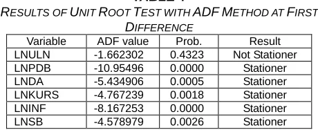
TABLE4
RESULTS OF UNIT ROOT TEST WITH ADFMETHOD AT FIRST
DIFFERENCE
Based on calculations using the ADF test at first different first showed that four variables: GDP, the budget deficit, the exchange rate and inflation is stationary, while the foreign debt is still stationary at first difference with the level of α = 5%. Thus do further testing using the ADF on the second difference.
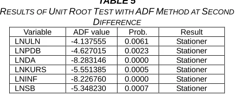
TABLE5
RESULTS OF UNIT ROOT TEST WITH ADFMETHOD AT SECOND
DIFFERENCE
Variable ADF value Prob. Result LNULN -4.137555 0.0061 Stationer LNPDB -4.627015 0.0023 Stationer LNDA -8.283146 0.0000 Stationer LNKURS -5.551385 0.0005 Stationer LNINF -8.226760 0.0000 Stationer LNSB -5.348230 0.0007 Stationer
Based on Table 5 shows that the entire value of the ADF showed that all variables are stationary at second difference and can be used in this study to analyze the short-term and long-term. After observation is believed that all variables have the same degree of integration, it can be tested cointegration of variables observation. The impact of an economic policy usually does not directly affect economic activity but take time or lag. Selection lag based on the Akaike Information Criterion (AIC) and Schawrz Info Criterion (SIC) to test the optimum lag absolt worth little and the highest adjusted R2 value.[16]So the selection of the optimum amount of lag is needed to obtain better results. Here are the results of calculation to obtain the optimum lag is right in the Engle-Granger cointegration test.[16]
TABLE6
RESULTS OF DETERMINING OPTIMAL LAG-LENGHT
Lag LogL LR FPE AIC SC HQ
0 -14.5958 NA 4.55e-07 2.4230 2.7171 2.4522 1 67.2766 96.3205* 2.81e-09* -2.9737* -0.9151* -2.7691*
The results of the test showed that the optimum lag which is used to test the Engle-Granger cointegration done using a long lag = 1. cointegration test is performed to determine whether there is a balance in the long term on the model chosen and established. In this study to test the cointegration using Engle Granger (EG) method. Basis for a decision is to compare the value of statistical DF with the critical value α = 0:05. If the statistical value is greater than the critical value then the observed variables mutually cointegrated or have a long-term relationship and if otherwise, then the observed variables are not cointegrated. From the estimation result can be seen in table 7 as follows:
TABLE7
RESULTS OF ENGLE-GRANGER COINTEGRATION Variabel Nilai Kritis DF
DF
ECT 1% 5% 10%
-2.692358 -1.960171 -1.607051 -2.578337
Table 7 shows that there is a long-term equilibrium relationship between cointegration testing on residuals (ECT) using the Dickey-Fuller (DF) model. If the value of DF statistics > critical value of DF is 5%, then it indicates cointegration between variables. The result obtained is the DF statistical value of -2.578337 > -1.960171 so that there is a cointegration between the variables of the regression results between gross
domestic product, budget deficit, exchange rate, inflation and interest rates on foreign debt. This indicates that the variable is said to be in a long-run equilibrium, so that the regression results are cointegrated regression. The ECM approach used in this study is the Error Correction Model Engle Granger approach. According to this approach, the ECM model is valid if the ECT coefficient sign is negative and statistically significant. After all variables are integrated, the next step is to perform an Error Correction Model regression. Error Correction Model is a technique for correcting short-term imbalances leading to long-term equilibrium.
TABLE7
REGRESSION ESTIMATION RESULTS USING THE ECMENGLE
-GRANGER METHOD
Variable Coefficient t-Statistic Prob. R-Squared
C 2.624287 3.312839 0.0161 0.944982
ECT(-1) -0.396846 -5.624829 0.0013 D(LNPDB,2) 0.030015 1.990276 0.0937 D(LNDA,2) 0.013842 2.161041 0.0740 D(LNKURS,2) 0.024989 0.448712 0.6694 D(LNINF,2) 0.070377 4.677258 0.0034 D(LNSB,2) -0.235302 -6.773833 0.0005 LNPDB(-1) -0.067745 -2.620920 0.0395 LNDA(-1) 0.053809 3.160511 0.0196 LNKURS(-1) -0.301672 -3.328529 0.0158 LNINF(-1) 0.133797 3.920139 0.0078 LNSB(-1) -0.093052 -2.222495 0.0680
The results of processing that have been carried out using the computer program E-Views 9.0, with the ECM linear regression model are shown in table 8. Error Correction of the Engle Granger Model shows that the coefficient value is negative and significant (probability value <absolute value critical value for α = 0.05). The coefficient value of ECT (Error Correction Term) is -0.396846 and the probability is 0.0013 <0.05. So the ECT coefficient value is negative and statistically significant means the Engle-Granger ECM specification model used in this study is valid.
Based on the results of the study in table 8, the ECM Engle Granger model short and long term is as follows:
D(LNULN) = 2.624287 + 0.030015 D(LNPDB,2) + 0.013842 D(LNDA,2) + 0.024989 D(LNKURS,2) + 0.070377 D(LNINF,2) - 0.235302 D(LNSB,2) - 0.067745 LNPDB(-1) + 0.053809 LNDA(-1) - 0.301672 LNKURS(-1) + 0.133797 LNINF(-1) - 0.093052 LNSB(-1) - 0.396846 ECT.
2423
Indonesia's foreign debt, the budget deficit with t-statistics = 3.160511 (prob = 0.0196 ) positive and significant effect on Indonesia's foreign debt, the exchange rate with tstatistics = -3.328529 (prob = 0.0158) has a negative and significant effect on Indonesia's foreign debt, inflation with t-statistics = 3.920139 (prob = 0.0078) has a positive effect and significant to Indonesia's foreign debt, and interest rates with tstatistics -2.222495 (prob = 0.0680) have a negative and not significant effect on Indonesia's foreign debt. Based on the estimation results in table 8, that in the short and long term the estimation results can be seen that the F-statistic value of 9.368616 with a statistical probability of 0.006163 is smaller than α = 0.05 indicating that together (simultaneous tests) all independent variables namely gross domestic product, budget deficit, exchange rate, inflation and interest rates have an influence on Indonesia's foreign debt. Based on the estimation results in table 8, the coefficient of determination (R2) obtained in the short and long term is 0.944982 or 94.4 percent, so that variations in gross domestic product, budget deficits, exchange rates, inflation and interest rates in the short term and the long term that is as big as 94.4 percent influences Indonesia's foreign debt. While the remaining 5.6 percent is explained by variables outside the model (which are not examined). The positive relationship between GDP and external debt in the short term is not in accordance with the monetarist theory but in accordance with the debt laffer curve theory which states that foreign debt is a normal requirement of every country, including Indonesia.[17] Foreign debt is needed at a reasonable rate. Economic growth as measured by GDP requires sufficient sources of development financing, one of which comes from foreign debt.[18] To accelerate economic growth, additional sources of financing derived from foreign debt are needed, so that with increasing GDP, greater sources of financing will be needed.[19] The addition of foreign debt will have a positive impact on GDP to a certain point or threshold.[20] The increase in foreign debt will be in line with the increase in the rate of return on foreign debt.[21] Furthermore, the government will utilize greater foreign debt to cover the repayment rate of the previous period. This can also be seen in the GDP and foreign debt data of 1998-2017 that there were several years when GDP experienced an increase followed by an increase in foreign debt in Indonesia. The insignificant effect is due to the fact that in the short term the increase in Indonesia's gross domestic income has not been significant enough to encourage an increase in foreign debt. The policy to increase foreign debt by the government is to channel these funds into infrastructure development and to stabilize the economy in Indonesia, which is classified as a developing country. Indonesia still has a dependency on other countries and because of the huge burden of foreign debt, where Indonesia not only pays principal debt installments but also pays so much debt interest. The budget deficit variable shows a positive but not significant relationship indicating that a country's budget deficit means a reduction in the budget to finance development and the Indonesian economy so that additional funding is needed. Foreign debt is one source of financing used as an alternative development financing by the government. But in the short term, when there is a budget deficit, the government needs funds relatively quickly so that the funds needed are not necessarily sourced from foreign debt, but can also be sourced from domestic funding such as by issuing state debt (bonds). The government also continues to increase state revenue each year through increased tax
investment in the country so that it can affect the decline in aggregate opinion.[23] This will cause a decrease in import capabilities. If the value of imports is lower than the value of exports (exports are greater than imports) it will cause a surplus in the current account so that it will reduce foreign debt. Therefore according to Keynesian theory that interest rates have a negative influence on foreign debt.[23] The insignificant effect of interest rates on foreign debt because interest rates cannot significantly affect Indonesia's foreign debt. The government will continue to increase foreign debt even though the benchmark interest rate in Indonesia has increased / decreased. Because in the short term the foreign debt is used by the government for spending in structural and sectoral sectors including health, education and infrastructure.
4 CONCLUSION
AND
RECOMMENDATION
Based on the estimation equation foreign debt in Indonesia by using models Error Correction Model Engle Granger, in the short term inflation and interest rates have a significant influence, whereas in the long term GDP, budget deficits, exchange rates and inflation which significantly, Bank Indonesia and the Government can adopt policies to maintain stable inflation, interest rates and the exchange rate so as to encourage an increase in the national income and reduce foreign debt. Restricting imports of goods from other countries and maximize the results from the source country of Indonesia. This will increase exports so that there is a surplus in the current account so that the foreign debt to be reduced. Reduce dependence on foreign debt by means of further enhancing the country's national income from taxes and natural resources and human resources of Indonesia.
REFERENCES
[1] F. Jaseviciene and E. Rudzionyte, ―Analysis of Budget Deficit and Its Problems in Lithuania,‖ Bull. Taras Shevchenko Natl. Univ. Kyiv Econ., no. 174, pp. 42– 51, 2015.
[2] H. W.-C. Yeung, ―Pol_Geog.pdf,‖ Polit. Geogr., vol. 17, no. 4, pp. 389–416, 1998.
[3] P. Alexakis, G. A. Hardouvelis, D. A. Paxson, G. Sick, and L. Trigeorgis, ―Greek Sovereign Debt: Addressing Economic Distress and Growth in the Euro Area,‖ SSRN Electron. J., pp. 1–33, 2018.
[4] N. Yoshino, P. Morgan, P. J. Morgan, and L. Q. Trinh, Frameworks for central–local government relations and fiscal sustainability, no. 605. 2017.
[5] O. Blanchard, ―Policy Options : Portugal and the Euro,‖ 2017.
[6] R. Greenhill, A. Prizzon, and A. Rogerson, ―The age of choice: developing countries in the new aid landscape A synthesis report Working Paper 364 Results of ODI research presented in preliminary form for discussion and critical comment Shaping policy for development,‖ Overseas Dev. Inst., 2013.
[7] J. Krishnakumar, M. J. Martin, and N. Soguel, ―Explaining Fiscal Balances with a Simultaneous Equation Model of Revenue and Expenditure: A Case Study of Swiss Cantons Using Panel Data,‖ Public Budg. Financ., vol. 30, no. 2, pp. 69–94, 2010.
[8] M. Adeolu and J. Sunday, ―Fiscal / Monetary Policy and Economic Growth in Nigeria : A Theoretical Exploration,‖ vol. 1, no. 5, pp. 75–88, 2012.
[9] B. Dafflon, ―Responsibility To Fiscal Discipline,‖ 2010.
[10] Z. M. Song, K. Storesletten, and F. Zilibotti, ―Rotten Parents and Disciplined Children: A Politico-Economic Theory of Public Expenditure and Debt,‖ SSRN Electron. J., 2011.
[11] E. Karagöl, ―The Causality Analysis of External Debt Service and GNP : The Case of Turkey,‖ Cent. Bank Rev., pp. 39–64, 2002.
[12] A. C. Arize, I. N. Kallianotis, S. Liu, J. Malindretos, and A. Panayides, ―National Debt and Its Effects on Several Other Variables: An Econometric Study of the United States,‖ Int. J. Financ. Res., vol. 5, no. 4, 2014. [13] M. Huchet-bourdon and J. Korinek, ―To What Extent
Do Exchange Rates and their Volatility Affect Trade ?,‖ OECD Trade Policy Work. Pap. Ser. No. 119, no. 119, pp. 1–36, 2011.
[14] F. Bayo, ―Determinants of Inflation in Nigeria : An Empirical Analysis,‖ Int. J. Humanit. Soc. Sci., vol. 1, no. 18, pp. 262–271, 1996.
[15] S. Abdelhafidh, ―External debt and economic growth in Tunisia,‖ Panoeconomicus, vol. 61, no. 6, pp. 669– 689, 2014.
[16] ―Gujarati, D. (2004) Basic Econometrics.pdf.‖ .
[17] S. G. Cecchetti, M. S. Mohanty, and F. Zampolli, ―The Future of Public Debt: Prospects and Implications,‖ SSRN Electron. J., no. 300, 2012.
[18] F. Kasidi and A. M. Said, ―Impact of external debt on economic growth : a case study of Tanzania,‖ Adv. Manag. Appl. Econ., vol. 3, no. 4, pp. 59–82, 2013. [19] L. Sulaiman and A. BA, ―Effect of External Debt on
Economic Growth of Nigeria,‖ vol. 3, no. 8, pp. 71–80, 2012.
[20] L. Drakes, C. Thomas, R. Craigwell, and K. Greenidge, ―Threshold Effects of Sovereign Debt: Evidence From the Caribbean,‖ IMF Work. Pap., vol. 12, no. 157, p. i, 2012.
[21] A. Korinek, ―Foreign currency debt, risk premia and macroeconomic volatility,‖ Eur. Econ. Rev., vol. 55, no. 3, pp. 371–385, 2011.
[22] M. Balcilar, A. M. Kutan, and M. E. Yaya, ―Testing the dependency theory on small island economies: The case of Cyprus,‖ Econ. Model., vol. 61, no. March 2016, pp. 1–11, 2017.